The Inuence of 2015-16 El Niño On the Record-Breaking Mangrove Dieback Along Northern Australia Coast
←
→
Page content transcription
If your browser does not render page correctly, please read the page content below
The In uence of 2015-16 El Niño On the Record- Breaking Mangrove Dieback Along Northern Australia Coast S. Abhik ( abhik.climate@gmail.com ) Bureau of Meteorology Pandora Hope Bureau of Meteorology Harry H. Hendon Bureau of Meteorology Lindsay B. Hutley Charles Darwin University Stephanie Johnson La Trobe University Wasyl Drosdowsky Bureau of Meteorology Josephine Brown University of Melbourne Research Article Keywords: in uence, Australia, investigates, climate, satellite, conditions, greenness variation Posted Date: June 28th, 2021 DOI: https://doi.org/10.21203/rs.3.rs-650667/v1 License: This work is licensed under a Creative Commons Attribution 4.0 International License. Read Full License
The influence of 2015-16 El Niño on the
record-breaking mangrove dieback along northern
Australia coast
S. Abhik1,* , Pandora Hope1 , Harry H.Hendon1 , Lindsay B. Hutley2 , Stephanie Johnson3 ,
Wasyl Drosdowsky1 , and Josephine Brown4,5
1 Bureau   of Meteorology, Melbourne, Australia
2 Research    Institute for the Environment and Livelihoods, Charles Darwin University, Darwin, Australia.
3 Department of Ecology, Environment and Evolution, La Trobe University, Bundoora, Australia.
4 School of Geography, Earth and Atmospheric Sciences, University of Melbourne, Melbourne, Australia.
5 ARC Centre of Excellence for Climate Extremes, University of Melbourne, Melbourne, Australia
* abhik.climate@gmail.com

ABSTRACT

This study investigates the underlying climate processes behind the largest recorded mangrove dieback event along the Gulf of
Carpentaria coast in northern Australia in late 2015. Capitalizing on the satellite observation-based mangrove green-fraction
dataset, variation of the mangroves during recent decades are studied, including their dieback during 2015. The relationship
between mangrove greenness and the climate conditions is examined using available observations and by exploring the
possible role of the mega 2015-16 El Niño in altering the favorable conditions for the mangroves. The mangrove greenness is
shown to be coherent with the low-frequency component of sea-level height variation related to the El Niño southern oscillation
(ENSO) cycle in the equatorial Pacific. The sea-level drop associated with the 2015-16 El Niño is identified to be the crucial
factor leading to the dieback event. A stronger sea-level drop occurred during austral autumn and winter, when the anomalies
were more than 12% greater than the previous very strong El Niño events. The persistent drop in sea-level height occurred in
the dry season of the year when sea-level was seasonally at its lowest, so potentially exposed the mangroves to unprecedented
hostile conditions. The influence of other key climate factors is also discussed, and a multiple linear regression model is
developed to understand the combined role of the important climate variables on the mangrove greenness variation.

1 Introduction
In late 2015, about 8,000 hectares of the forested tidal wetland along a 1000 km stretch of the coastline of Australia’s Gulf of
Carpentaria (see figure 1a for its location) experienced an extensive dieback of its mangroves1–3 . Mangroves are an important
part of the local ecosystem, providing habitat for many marine and coastal species, protecting coastlines from extreme weather
and erosion, filtering out sediment from river run-off to protect seagrass, as well as absorbing substantial amounts of greenhouse
gases4–6 . Because of their ecological importance, considerable attention has been paid to this dieback event to understand
its extent, cause, and severity7–9 . Mangrove dieback events were also observed during 2015-2016 in Kakadu National Park,
Northern Teritory10 and in a semi-arid stand near Exmouth, Western Australia11 , but those events were not as extensive and
severe as the Gulf of Carpentaria mangrove dieback. Preliminary observations have ruled out any direct influence of human
activities (e.g., oil spills), pathogens or any extreme weather event (e.g., tropical cyclone) at this time. Thus the prevailing
climate conditions, possibly driven by the mega-El Niño that occurred during 2015-16, might be the primary factor for the
dieback1, 12 , but the precise connection with the climate drivers has not previously been identified.
     Mangroves exhibit wide physiological tolerance and can intake fresh groundwater as well as saline water during tidal
inundation13, 14 , thus they can withstand a wide range of daily and seasonal tidal variations. However, a major departure from
the usual hydrological regime can induce physiological stress to the mangroves and their spatial extent may be considerably
modified11, 15 . Earlier studies have suggested a range of climatic factors that might be important in causing stress to the
mangroves, including unusually high temperatures, below-normal rainfall and humidity, and sustained low sea-level1, 12 . Harris
et al.16 described the 2015 event as a climatic ‘press-pulse’ process, with a long-term, slow climatic press changing the
climatic envelope ecosystems are adapted to, with the impact of this press amplifying the extreme of pulse events. Overlaid
on an ongoing warming trend associated with global warming, It is suggested that the ‘pulse’ was not sudden for the Gulf
mangrove dieback but comprised a sustained months-long drop in sea-level due to the 2015-16 El Niño12 , and enhanced air
temperatures with persisting drought condition acting to limit freshwater input to the coastline. Owing to their shallow roots,

                                                                1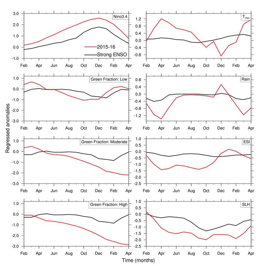
two mangrove species, particularly Avicennia marina and to a lesser extent Rhizophora stylosa are vulnerable to prolonged
below normal sea-levels. Sippo et al.17 concluded that dry conditions combined with porewaters enriched in iron associated
with unprecedented below-normal sea levels were the potential causes of the dieback. As a result of months-long episode or
permanent sea level drop, a change in the ecosystem can be triggered, with a shift from mangrove forest to drier and more
saline saltmarsh, where only a few specialised plants can only grow18 .
    Sea level drop is possibly a major issue in the dry season, when this stress factor is compounded by persistent low rainfall19 .
However, mangroves are reasonably heat tolerant20 and the Gulf mangroves routinely cope with the dry season every year.
Furthermore, they have apparently remained mostly unaffected during other El Niño events in the recent past, even during
previous strong El Niños such as 1997-981 . This evokes the questions: what was unusual about the 2015-16 El Niño that
resulted in the massive dieback? Was it simply its magnitude, or was the timing and possibly co-occurrence with other climatic
factors crucial? Any effort to address these outstanding questions will help in understanding how this environmental catastrophe
occurred and should facilitate improved capability for monitoring and prediction, which promises great value in the optimization
of risk management for policymakers, rangers, and communities in the future.
    In this study, we examine the climate conditions during the 2015-16 El Niño in the context of conditions during previous El
Niño events. We utilise satellite-based mangrove greenness observations to investigate the greenness changes associated with
variations of observed sea level height (SLH), rainfall, surface air temperature, and a measure of vegetation moisture stress
formed by comparing potential and actual evapotranspiration. Based on the observed mangrove variations during previous
El Niño events and any associated droughts and heat extremes, we provide a plausible explanation for the 2015 dieback that
points at the un-fortuitous seasonal timing and magnitude of the 2015-16 mega El Niño as the primary culprit. We also derive a
statistical relationship between mangrove changes and SLH, temperature and evapotranspiration variations to provide a stress
index model that can be used to anticipate variations of mangroves associated with variations of climate conditions in the future.

2 Data & Method
The mangroves of the Gulf of Carpentaria coast typically grow in a narrow 100-200m span along the shoreline, and thus
require high-resolution data for effective monitoring. The satellite-based Landsat Thematic Mapper (TM), enhanced TM
and operational land imager provide a reasonably high spatial resolution (30m) observation of mangrove greenness every
16 days (cloud permitting) since late 1980s21 . The vegetation sampling sites are randomly positioned within the maximum
historical extent of the mangroves (figure 1a), as mapped by the Mangrove canopy cover version 2.0.222 . Plots, 90 × 90 m,
are stratified to represent three distinct mangrove communities: estuarine, hinterland, tidal, and three dieback classes based
on the green-fraction reduction during 2015-16: high (80-100%), moderate (60-79%), and low (30-59%). Dieback severity
is classified based on relative cover loss between pre-dieback (preceding dry season of 2015) to post-dieback (following wet
season of 2015-16). All sites are spaced a minimum of 500m apart unless areas are of different severity classes. Fractional
cover products are derived by separating pixels into constituent fractional exposed greenness cover using spectral unmixing
algorithms with joint remote sensing research program23 . We extract fractional cover scenes by removing pixels influenced by
cloud, cloud shadow, and surface water, using bitwise masking “Water Observation Feature Layers" derived from the Water
Observation from Space24 . A mean monthly green-fraction is derived for each site from all available fractional greenness
coverage observations from 1987 to 2020. The outliers are excluded from the time series using a rolling mean to detect data
points that exceeded more than 20% cover change from the three-month average. All fractional cover products are extracted
using Digital Earth Australia’s sandbox platform25 , and the products accessed from the open data cube26 .
    SLH variations are monitored with observations from the Australian Bureau of Meteorology (BOM) Milner Bay, Groote
Eylandt tide-gauge station (location shown in figure 1a) during 1993-2018. As the seasonal cycles of the SLH are similar
across all the stations in Gulf of Carpentaria27, 28 , it is reasonable to use a single tide-gauge location as representative of
SLH in the Gulf of Carpentaria. We also utilize monthly Bluelink ReANalysis (BRAN) SLH analyses29 , which are available
globally between 75◦ S − 75◦ N at 10km resolution. BRAN assimilates observations of SLH (based on satellite altimetry and
in situ observations) together with in situ observations of temperature and salinity into a global ocean model using ensemble
optimal interpolation of observational data assimilation system to provide several 3-dimensional time-varying analyses of ocean
temperature, salinity, currents and SLH.
    Monthly rainfall and maximum surface air temperature (Tmax ) dataset on 0.05◦ grid are obtained from the Australian Water
Availability Project (AWAP)30 . This data is available across continental Australia back to 1911. We use monthly surface zonal
wind analyses from European Centre for Medium-Range Weather Forecasts (ECMWF) Interim reanalysis (ERA-I)31 , which
are available globally on a 1.5◦ grid during 1979-Aug 2019. An evaporative stress index (ESI)32, 33 is used to examine the
evaporative stress along the Gulf’s coast. This index is the normalized ratio of evapotranspiration to potential evapotranspiration,
which are derived from the outputs of the AWRA-L landscape water balance model over Australia (version 6) and is indicative
of surface moisture supply and evaporative demand34 . The rainfall, Tmax and ESI data are averaged over coastal Gulf region
(shown as red box in figure 1a).

                                                                                                                               2/16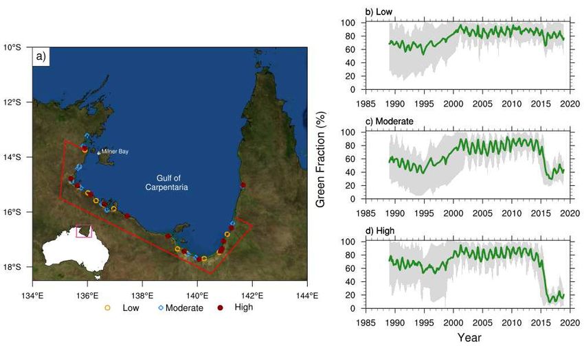
The anomalies are calculated by removing the seasonal cycle (time mean and first three harmonics of climatological annual
cycle) from the variable and the linear trends are removed from the anomalous timeseries. The anomalies are standardised
by their own standard deviation to obtain the normalised anomalies. We identify previous strong El Niño events as when the
oceanic Niño3.4 index exceeds 1.5 standard deviations in the November-January season, when El Niño conditions typically
peak in cenntral to the eastern equatorial Pacific. This Niño3.4 index is an average of sea surface temperature (SST) over the
central Pacific region (5◦ S − 5◦ N, 170◦W − 120◦W ), calculated using HadISST dataset35 . To increase the sample size of strong
El Niño events, we assume linearity of La Niña events (being opposite to El Niño) and include in our composite of the previous
strong La Niña events but flip the sign of the anomalies. Based on this index, we identify the austral summers of 1957-58,
1965-66, 1972-73, 1982-83, 1987-88, 1991-92, 1997-98, 2015-16 as strong El Niño years and 1973-74, 1975-76, 1988-89,
1998-99, 1999-2000, 2007-08, 2010-11 as strong La Niña years. The Interdecadal Pacific Oscillation (IPO) is monitored using
SST-based IPO tripole index (TPI)36 .

3 Results
Historical perspective of the mangrove green-fraction variability
The monthly timeseries of the mangrove greenness in the three dieback categories for over 30 years are displayed in figure
1b-d. The green-fraction dataset is averaged over all the sites in each category and the mean monthly green-fraction timeseries
with its range across the sites are shown. A substantial drop in green-fraction is evident for the moderate and high dieback
categories during 2015, with some locations in the high category experiencing near 100% loss of greenness. However, abundant
variability is also evident, primarily associated with the seasonal cycle (greenness peaks in austral autumn), but also with other
low-frequency variations. For instance, the green-fraction has a sustained 20% reduction around 1994 and subsequent recovery
during the late 1990s. However, the magnitude of the drop during 2015 is unprecedented at least in the last few decades
(e.g., Duke et al.1 ). The seasonal variation of the mangrove greenness is ∼10% of the mean, with the maxima occurring in
March-April and the minima around October (figure S1). During 2015, the seasonal reduction of green-fraction started about a
month or two before the climatological minima and it dropped noticeably for moderate and high categories by Aug-Sep.

Impact of El Niño events
Considering the coincidence of the strong El Niño of 2015-16 with the 2015 dieback event, we examine the variation of different
climate variables during the 2015-16 El Niño and compare them with previous strong El Niño conditions. This provides a
paradigm for understanding the extreme climate conditions that might have stressed the mangroves during 2015-16. Figure 2
shows the evolution of the normalized Niño3.4 index, mangrove green-fraction, Tmax , rainfall, ESI along the Gulf coast and
SLH anomalies at Milner Bay from the development period of the strong El Niño events (the preceding February) to their
demise (the following April). The influence of strong El Niños on the variables are obtained by lag-regressing the normalised
anomalies onto December Niño3.4 index and the derived regression coefficients are scaled by the normalised Niño3.4 index
magnitude (1.44) during strong ENSO. SST in the Niño3.4 region of the eastern equatorial Pacific tends to peak in December.
Mangrove green-fraction reduces after the peak of El Niño events, but this reduction in greenness is not usually large. During a
typical El Niño event, Tmax in the Gulf region is near to neutral in the development stage and then becomes higher than normal
at the peak of El Niño (i.e., during December-February). For this Gulf region, rainfall displays little variation during El Niño,
however evaporative stress is typically stronger than normal (i.e., negative anomalies) throughout the course of El Niño. Finally,
SLH in the Gulf is also seen to be typically lower than normal from late winter through to early autumn, consistent with the
strong influence of the Pacific on the Gulf SLH variation as revealed in Oliver and Thompson28 .
    During the 2015-16 El Niño, the Niño3.4 SST index was 50% stronger at its peak in December 2015 compared to the
composite. It started to become positive earlier since the preceding austral winter and lasted later into the following autumn.
A strong positive Tmax anomaly developed around April-May, but it reversed sign during the peak of the event in December
2015. Lower than normal rainfall accompanied the high Tmax in the preceding winter, but rainfall was near normal during the
peak of the event during spring and early summer 2015, consistent with the weak rainfall anomalies observed during previous
strong El Niño events. And, in contrast to other El Niño events, ESI was very negative in the autumn, winter and spring of
2015, indicating persistence of a stressful environment for the mangroves. Lastly, SLH became much lower than normal 4-5
months earlier than is typically observed during El Niño and remained lower longer into the following autumn. The de-trended
SLH time-series at Milner Bay indicates that the drop during 2015 was unprecedented. From this cursory analysis, the extreme
drop in SLH together with the preceding strong increase in negative ESI and high Tmax during the preceding winter could
have provided the necessary stress to cause the extreme dieback that was sustained during 2015 (figure 2). The persistent
below-normal SLH especially during hot and dry conditions would have resulted in limited tidal mixing and that might provide
a stressful condition for the mangroves, which generally intake water during tidal inundation14 .

                                                                                                                             3/16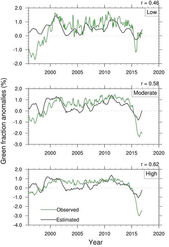
Connections between mangrove greenness and climate variables
We further explore the historical relationship between SLH and mangrove greenness and their association with El Niño
conditions in the equatorial Pacific using cross-spectral analysis between SLH and green-fraction. This analysis is useful for
quantifying the relationship between two variables as a function of frequency and estimating their phase relationship. We
compute the coherence squared by Fourier transforming the deseasonalized monthly times series for 1994-2016, which provides
a band width of 1/276-month−1 . The coherence squared is formed after smoothing the raw power and cross power estimates
with a 9-point box car, yielding an effective bandwidth of 9/276 month−1 .
The top panels of figure 3 show the coherence squared and phase lag between the monthly SLH at Milner Bay and the
index of mangrove green-fraction for three dieback categories. The cross-spectra are found to be largely similar for all three
categories - the peak coherence up to 0.45 occurs around 0.03-month−1 frequency (period ∼2.8 years) and are broadly high for
frequencies lower than 1/25 month−1 (period ∼2.1 years). There are no other significant spectral peaks at higher frequencies.
The phase lag (about 45◦ ) indicates that low frequency (period longer than 2 years) greenness variation lags SLH by about 5-6
months, which is reasonable as it should take a few months for the mangroves to react to lower or higher than normal sustained
SLH change.
A similar quantification of the relationship between Gulf’s mangrove green-fraction and coastal Gulf region area averaged
ESI is shown at the bottom panels of figure 3. A weaker spectral peak at periods longer than 2 years is also evident with
about 3-4 months phase lag. We also examine the coherence-squared between green-fraction and Tmax , and rainfall (figure S2)
and unlike SLH and ESI, these variables generally show no significant coherence with greenness. Only the peak coherence
between Tmax and green-fraction for moderate and high dieback categories at the frequencies lower than 24 months is found to
be marginally significant (p=10%). An out-of-phase relationship is also noted between green-fraction and Tmax , indicating
reduction of green-fraction due to low frequency warming over the Gulf.
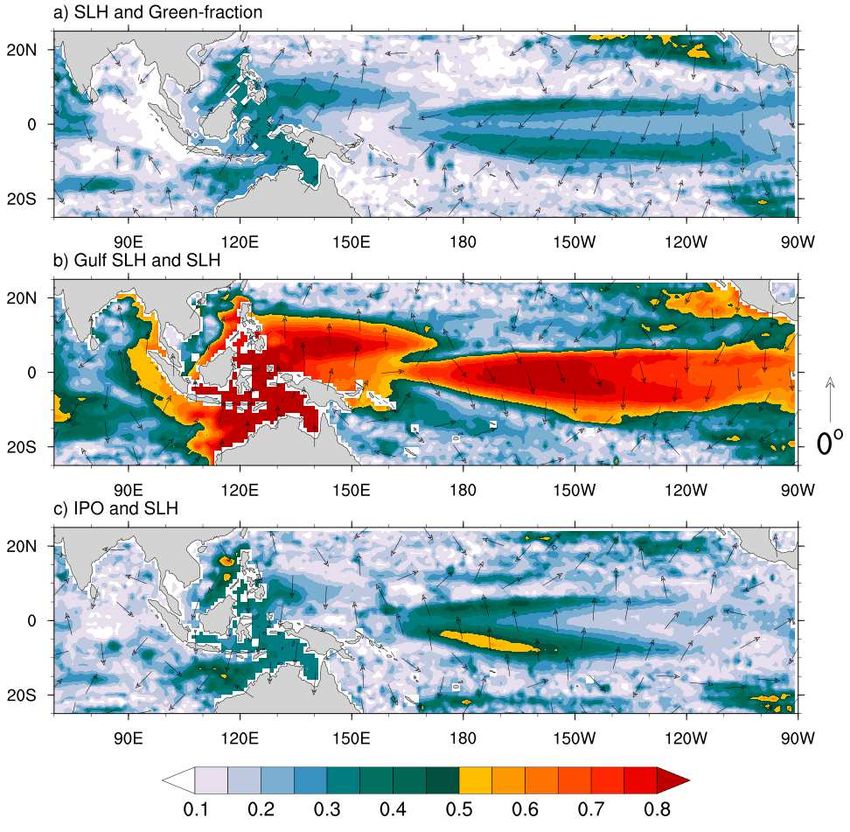
More insight into the cause of the low frequency SLH anomalies associated with greenness variations is gained by examining
the spatial distribution of the coherence-squared between the gridded BRAN SLH and mangrove green-fraction index anomalies.
The coherence-squared and phase lag for the dominant low frequency band around the 30-month cycle are shown in figure
4a. Here we form the index of greenness by averaging standardized greenness anomalies. Mangrove greenness at Gulf
of Carpentaria sites is coherent with SLH throughout the Gulf and on the north-west coast of Australia, in the seas of the
Indonesian archipelago and in the north-west Pacific, with a constant phase lag of about 1/8 cycle (∼4 months). The greenness
is also found to be coherent with SLH on the equatorial central and eastern Pacific, with a distinctive horse-shoe pattern. The
phase is roughly 180◦ shifted from that in the Gulf and surrounding seas, indicating that greenness is coherent with an El
Niño-like fluctuation of SLH (i.e., low SLH in the Gulf and western Pacific coincides with high SLH in the central and eastern
Pacific). However, the pattern of coherence in the central and eastern Pacific, with its distinctive horseshoe shape, is more
indicative of the interdecadal variation of ENSO referred to as the IPO (e.g., Power et al.37 ). This sensitivity of greenness to
the lower frequency component of ENSO presumably arises for two reasons. First, the lower frequency component of ENSO
drives a stronger variation of SLH in the Gulf than it does by the typical interannually varying El Niño event. This is confirmed
by examining the coherence of SLH in the Gulf with SLH at every grid point for the dominant frequency band (figure 4b).
The peak coherence with SLH in the eastern Pacific, which has the opposite phase to that in the Gulf, occurs just east of the
dateline and with a relative minimum in coherence along the equator in the eastern Pacific. This is a typical IPO feature and the
coherence between the IPO index and SLH confirms this structure (figure 4c). Secondly, as greenness is effectively a slowly
varying parameter, it is more coherent with the lower frequency components of El Niño. These two processes together result in
a pattern of coherence between greenness and SLH that looks more like the IPO than it does El Niño. That is, greenness is
more responsive to the low-frequency tail of ENSO variability than it is to the higher frequency interannual components.
The overall pattern of coherence of SLH with greenness thus reflects the spatial structure of ENSO, suggesting that the El
Niño driven SLH variability is linked with mangroves. During El Niño, westerly wind anomalies in the western Pacific act to
elevate the SLH to the east with a Kelvin wave structure and lower SLH in the western Pacific with Rossby wave structure38 .
The lower SLH anomalies in the west Pacific travel through the Indonesian seas and act to lower the SLH in the Gulf28 and
down the west coast of Australia where it is transmitted as a coastally trapped Kelvin wave39 . The broader meridional structure
of the SLH variation in the central and eastern Pacific is coherent with Gulf greenness and that reflects the structure of the lower
frequency tail of El Niño, and it is associated with slower westward propagating Rossby waves off the equator in the eastern
and central Pacific. However, it remains in question why the mangroves dramatically declined in 2015 but survived during other
El Niño events. We explore this outstanding question by examining SLH variation during strong El Niños next.
Sea level variation during strong El Niños – how did 2015-16 differ?
To gain insight into the SLH variation during El Niños, we look at the timing of the SLH decline during 2015-16 and compare
that with other strong El Niño events. Figure 5a displays the annual cycle of SLH in Milner Bay along with the variations
during 2015-16 and two other strong El Niño events (1982-83 and 1997-98). The SLH maximum occurs during austral summer
4/16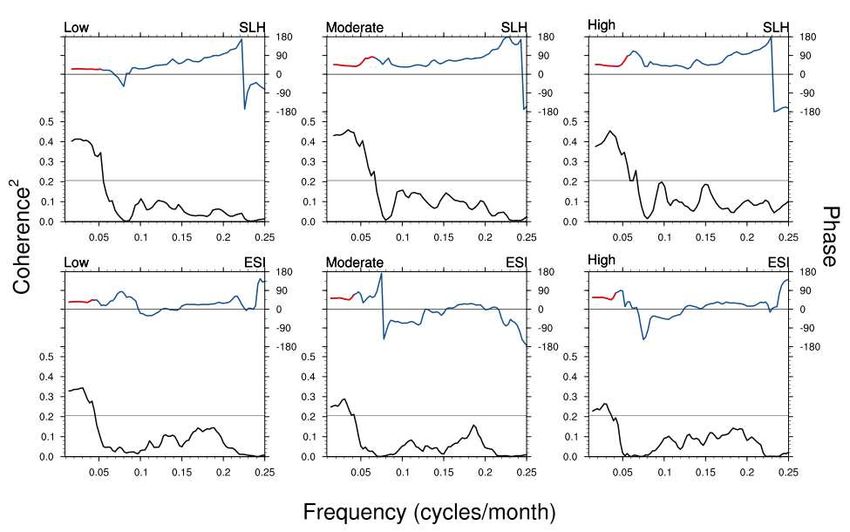
and the minimum is noted during late winter. Forbes and Church27 explained seasonal SLH variation as a result of the seasonal
cycle of wind stress over the region (i.e., westerlies during the summer monsoon acting to raise SLH and peak easterly trade
winds during winter that act to lower SLH). The three El Niño events shown in figure 5a result in lower-than-normal SLH from
about April of the year El Niño commences through to the following March. But it is noted that no severe mangrove dieback
was recorded during the 1997-98 El Niño event, which has been referred to as “El Niño of the century" for its extraordinary
magnitude and influence on the global weather and climate40 . The most dramatically different behaviour of the 2015-16 El
Niño is the much stronger negative SLH anomalies during austral autumn and winter, when the anomalies were more than 12%
stronger than the previous two very strong El Niño events. The extreme sea level decline in 2015 coincided with the seasonal
minimum, so potentially exposed the mangroves to unprecedented low SLH.
The extremity of the low SLH during 2015 is quantified by computing the cumulative deficit of detrended SLH. We do this
both for the cumulative anomaly and for the cumulative anomaly below the climatological minimum, which is assumed to be
the threshold below which the mangroves cannot be sustained. We show this for the 1997-98 (figure 5b) and 2015-16 (figure
5c) El Niño events. This analysis indicates that cumulative stress due to below-normal SLH was double in 2015-16 compared
to 1997-98. Sustained SLH below the climatological minimum continued into October 2015 but was confined to only moderate
values during June-August 1997.
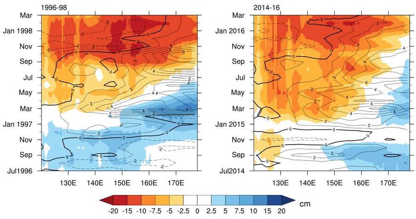
We further evaluate the SLH and surface zonal wind evolution around the equatorial Pacific during the strong El Niño events
of 1997-98 and 2015-16 (figure 6). This domain was chosen as the onset of the wind anomalies occurs along the equator41
and the wind-forced SLH changes in the equatorial western Pacific appear to have a strong relationship with the Gulf’s SLH
variation. Figure 6 indicates that the drop in SLH around the equatorial Pacific during peak El Niño months of 1997-98 were
stronger relative to the same period of 2015-16. But during early and middle months of 2015, the SLH drop was greater
compared to the same period in 1997. The below-normal SLH anomalies during 2015 can be traced back to mid-2014, when
an El Niño event false-started42 . As the westerly zonal wind anomalies strengthened around late austral autumn of 2015, the
wind-induced downwelling Kelvin wave acted to lower SLH in the western Pacific for a prolonged period in early and middle
months of 2015, especially in the dry season of the year.
Our analysis suggests that the low-frequency (periods longer than 2-3 years) SLH is the key driver of the mangrove dieback
event. A persistent drop in SLH associated with El Niño likely establishes a stressful environment for the mangroves, especially
during the dry months of the year (late austral autumn and winter). Additionally, evaporative stress, as quantified by the ESI,
appears to be important for the mangroves as does Tmax . The 2015 El Niño was thus catastrophic because SLH dropped
considerably much earlier than usually occurs during El Niño. It exposed the mangroves to a sustained period of SLH well
below its climatological minimum, together with atmospheric anomalies that resulted in increased evaporative stress during the
preceding autumn and winter seasons. This sustained low relative sea-level was captured by the mangrove stress index defined
in Duke et al.3 . In this study, we go further and include other potential factors to derive a mangrove stress index.
Mangrove stress index
To understand the combined role of the potential climate variables on the dieback event, we reconstruct the mangrove green-
fractions for each of the dieback categories using SLH, ESI and Tmax anomalies. A multiple linear regression model is developed
to estimate the greenness variations with seasonal cycle removed, detrended, standardised 6-month lagged SLH at Milner Bay,
3-month lagged ESI, and Tmax anomaly time-series over the coastal region of the Gulf as the predictors. A 12-monthly running
mean is applied to the predictors to eliminate the high-frequency variability. The mathematical model for the multilinear
regression analysis is as follows:
Green f ractionestimated = b0 + b1 .SLH + b2 .ESI + b3 .Tmax (1)
The estimated and observed green-fractions for three dieback categories over the period of 1994-2018 are displayed in
figure 7 and the associated regression coefficients with relevant statistics are given in Table 1. Consistent with our previous
results, SLH has the dominant contribution, and the associated coefficients are significant at the 5% level for all three categories.
By contrast, temperature and ESI show weaker association and the regression coefficients for the Tmax anomalies are not
significant at the same confidence level.
The correlations between estimated and observed green-fractions range between 0.47 and 0.62. Relatively higher correlations
are noted for the high dieback, suggesting adequate skill of the regression model in predicting the vulnerable mangroves. The
reconstructed green-fractions also show an unprecedented reduction in greenness during 2015, though the estimated decrease is
much weaker than observed. Nevertheless, the analysis in figure 7 confirms that the multilinear regression model can be used to
construct the mangrove stress index for estimating the future condition of the mangroves using dynamical seasonal forecasts
(e.g., Long et al.43 ) and climate model projections, and it will form the focus of future work.
5/16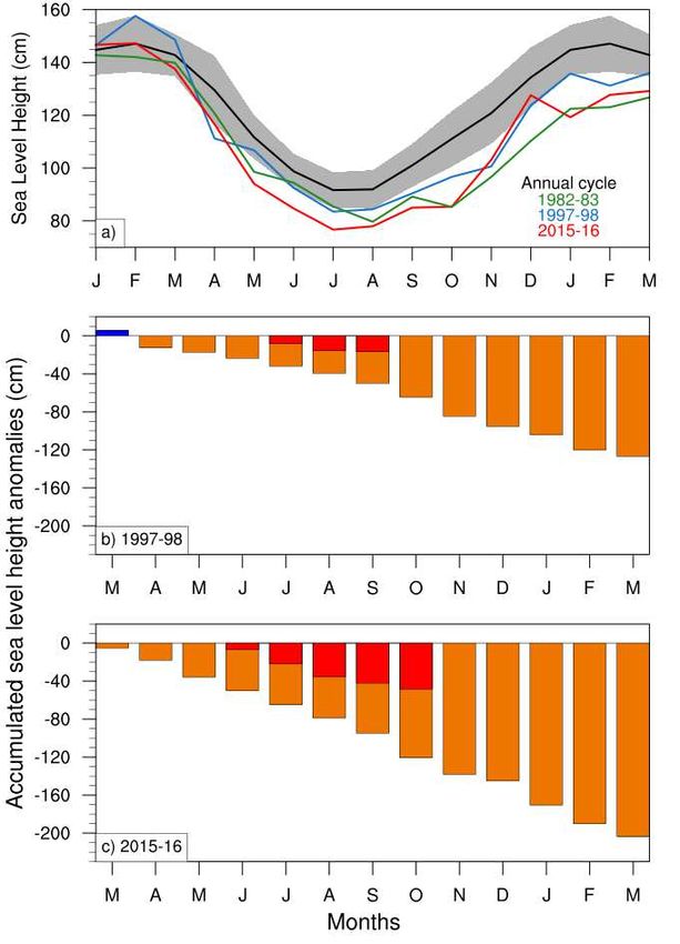
Table 1. Regression coefficients for three dieback categories during 1994-2018 from the multiple linear regression model (1).
Regression coefficients significant at 5% level are marked in bold.

                                       Dieback class     Regression Coefficients
                                                         b0       b1       b2       b3
                                       Low               0.151    0.427    0.386    -0.076
                                       Moderate          0.377    0.606    0.12     -0.089
                                       High              0.216    0.604    0.325    -0.087

4 Discussion
We investigate the climate conditions during the 2015 mangrove dieback event along the southern coastline of the Gulf of
Carpentaria using available observations and reanalysis datasets. The decline in SLH associated with the positive phase of
ENSO is shown to be primarily responsible for the dieback event. The eastward shift of the equatorial Walker circulation
during El Niño drives a dynamical drop in sea level throughout the Gulf of Carpentaria, which exposes the mangroves to hostile
conditions. Our analysis over the period 1994-2018 suggests that low-frequency SLH variability (i.e. a period longer than 2
years) associated with ENSO explains about 50% variation of the observed low frequency variation of mangrove green-fractions.
Slowly varying greenness is shown to be more strongly associated with the lower frequency (decadal) component of ENSO
than its higher frequency interannual components.
     The phase lag between SLH change and the variation of mangrove greenness (greenness declines after SLH drops) indicates
that green-fraction reduces about 5-6 months after the persistent drop in SLH. During 2015, a much stronger SLH drop, about
12% greater than previous strong El Niño events, and much earlier onset of the decline (SLH dropped in June-July 2015
whereas typical SLH drop during El Niño does not occur until Aug-Sep) occurred during June-July when SLH is seasonally at
its lowest, and that potentially exposed the mangroves to unprecedented conditions. A prolonged period with low SLH along
with stronger dry and warmer conditions during a typical El Niño provided a stressful environment for the mangroves. Such
hostile conditions during 2015 caused canopy loss of the mangroves and eventually led to the massive dieback event.
     The drop in SLH in the Gulf in 2015 was also associated with a drop in SLH along the western Australia coast, which
typically occurs during El Niño. This decline in SLH was also responsible for a relatively small-scale mangrove dieback event
along the Western Australia coast11, 44 , reflecting the rapid adjustment of SLH along the north and west coasts of Australia
in response to El Niño (e.g., Potemra45 ). The below normal SLH that began in 2014 due to weak El Niño condition in that
year were further lowered in early and middle months of 2015 by the strong westerly wind anomalies around the equatorial
western Pacific leading to critically below-normal SLH in the Gulf of Carpentaria during the dry season of 2015. The dynamical
mechanism for the remote response of sea level during El Niño in the Gulf (e.g. Oliver and Thompson28 ), along the western
Australia coast is well established and what set the 2015 El Niño apart from previous events, in addition to its strong amplitude,
was its early onset.
     The severity of the 2015 mangrove dieback in the Gulf of Carpentaria is found to differ with geographical location, primarily
due to distance to the shoreline, local elevation, and distance from the creek2, 3 . While the previous existence of the mangroves
has been noted at a few of the locations in our study, mangroves have apparently emerged since the mid-90s at many of the
locations, perhaps in response to the rising SLH. There is a detectable impact of the 1997-98 El Niño on the green-fraction at a
few sites, causing ∼20-40% loss of greenness of the mangroves. In contrast, some of the plots are almost unaffected in the last
few decades, even during the 2015-16 dieback event. Some of those plots that have not sustained extensive dieback in 2015, is
a frontal stand dominated by Rhizophora stylosa, while other unaffected plots are in a relatively broad and lush region next to a
tidal creek. The rest of the dieback plots are at least a few meters (60-200 m) away from the shoreline and having little elevation
from the mean SLH. These contrasting patterns of dieback at fine-scales emphasise the importance of hydro-geomorphic setting
(height above mean SLH, distance to drainage channels) and hydroperiod (duration of tidal inundation) as important factors
that determine the severity of the dieback. An assessment of the plot-scale geomorphic variation is beyond the scope of this
present study.
     It may be inferred from our analyses and assessment of Duke et al.1 that the 2015 mangrove dieback event was primarily
driven by large-scale stressors (e.g., decadal ENSO variability), however, regional variation of mangrove species, inundation
period, distance to drainage channels influenced extent of the dieback. This motivates further investigation using high-resolution
green-fraction dataset across the dieback locations to explore the small-scale variation of the dieback event. As the global

                                                                                                                             6/16
climate warms46 , and features of ENSO may change47 , mangroves are likely to experience further stress (e.g. Sippo et al17 ).
Future investigation could include an examination of changes in the large-scale climate stressors in climate model projections to
determine if there is an increased likelihood of experiencing mangrove stress events similar to 2015 in the Gulf of Carpentaria
in a warming climate.
Acknowledgments
This work is funded by the Northern Territory Government, Australia. We are indebted to Norman Duke, Tony Griffiths, Ruth
Reef, Marycarmen Martinez Diaz, Grant Staben for stimulating discussions during the course of this study. We would like to
thank Claire Spillman, Matthew Wheeler, S. Sharmila for their constructive comments, which greatly helped to improve this
manuscript. Thanks to Hanh Nguyen for providing ESI dataset. AWAP Tmax , rainfall, and Milner Bay tidal gauge observations
are accessed from BOM climate data server. BRAN SLH dataset is made freely available by Commonwealth Scientific and
Industrial Research Organisation (CSIRO) Bluelink and is developed in a collaboration between the Australian Department of
Defence, BOM and CSIRO : http://dapds00.nci.org.au/thredds/catalog/gb6/BRAN/BRAN_2016/alt_sea_level/catalog.html.
ERA-Interim reanalysis data are obtained from ECMWF: http://eccharts.ecmwf.int/datasets/. The analyses were performed
using the NCAR Command Language: https://doi.org/10.5065/D6WD3XH5.
References
1. Duke, N. C. et al. Large-scale dieback of mangroves in Australia’s Gulf of Carpentaria: a severe ecosystem response,
coincidental with an unusually extreme weather event. Marine and Freshwater Research 68.
2. Duke, N. C. et al. Assessing the Gulf of Carpentaria mangrove dieback 2017–2019 1, 226
(2020). URL https://nesptropical.edu.au/wp-content/uploads/2021/05/Project-4.
13-Final-Report-Volume-1.pdf.
3. Duke, N. C., Mackenzie, J., Hutley, L., Staben, G. & Brouke, A. Assessing the Gulf of Carpentaria mangrove
dieback 2017–2019 2, 150 (2020). URL https://nesptropical.edu.au/wp-content/uploads/2021/
05/Project-4.13-Final-Report-Volume-2.pdf.
4. Gilman, E. L., Ellison, J., Duke, N. C. & Field, C. Threats to mangroves from climate change and adaptation options: a
review. Aquatic botany 89, 237–250 (2008).
5. Lovelock, C. E. et al. The vulnerability of Indo-Pacific mangrove forests to sea-level rise. Nature 526, 559–563 (2015).
6. Jeffrey, L. C. et al. Are methane emissions from mangrove stems a cryptic carbon loss pathway? insights from a catastrophic
forest mortality. New Phytologist 224, 146–154 (2019).
7. Slezak, M. Massive mangrove die-off on Gulf of Carpentaria worst in the world, says expert. The Guardian 11 (2016).
8. Wild, K. Shocking images’ reveal death of 10,000 hectares of mangroves across Northern Australia. Australian Broadcasting
Corporation (2016).
9. Van Oosterzee, P. & Duke, N. Extreme weather likely behind worst recorded mangrove dieback in northern Australia. The
conversation 14, 1–6 (2017).
10. Asbridge, E. et al. Assessing the distribution and drivers of mangrove dieback in Kakadu National Park, northern Australia.
Estuarine, Coastal and Shelf Science 228, 106353 (2019).
11. Lovelock, C. E., Feller, I. C., Reef, R., Hickey, S. & Ball, M. C. Mangrove dieback during fluctuating sea levels. Scientific
Reports 7, 1–8 (2017).
12. Harris, T. et al. Climate drivers of the 2015 Gulf of Carpentaria mangrove dieback (2017).
13. Ball, M. C. Ecophysiology of mangroves. Trees 2, 129–142 (1988).
14. Lovelock, C. E., Reef, R. & Ball, M. C. Isotopic signatures of stem water reveal differences in water sources accessed by
mangrove tree species. Hydrobiologia 803, 133–145 (2017).
15. Eslami-Andargoli, L., Dale, P., Sipe, N. & Chaseling, J. Mangrove expansion and rainfall patterns in Moreton bay, southeast
Queensland, Australia. Estuarine, Coastal and Shelf Science 85, 292–298 (2009).
16. Harris, R. M. et al. Biological responses to the press and pulse of climate trends and extreme events. Nature Climate
Change 8, 579–587 (2018).
17. Sippo, J. Z. et al. Reconstructing extreme climatic and geochemical conditions during the largest natural mangrove dieback
on record. Biogeosciences 17, 4707–4726 (2020).
7/1618. Goudkamp, K. & Chin, A. Mangroves and saltmarshes (2006).
19. Ball, M. Mangrove species richness in relation to salinity and waterlogging: a case study along the Adelaide River
floodplain, northern Australia. Global Ecology & Biogeography Letters 7, 73–82 (1998).
20. Medina, E. Mangrove physiology: the challenge of salt, heat, and light stress under recurrent flooding. Ecosistemas de
manglar en América tropical 109–126 (1999).
21. Wulder, M. A. et al. The global Landsat archive: Status, consolidation, and direction. Remote Sensing of Environment 185,
271–283 (2016).
22. Lymburner, L. et al. Mapping the multi-decadal mangrove dynamics of the Australian coastline. Remote Sensing of
Environment 238, 111185 (2020).
23. Scarth, P., Guerschman, J. P., Clarke, K. & Phinn, S. Validation of Australian fractional cover products from MODIS
and Landsat data. AusCover Good Practice Guidelines: A Technical Handbook Supporting Calibration and Validation
Activities of Remotely Sensed Data Product 123–138 (2015).
24. Mueller, N. et al. Water observations from space: Mapping surface water from 25 years of Landsat imagery across
Australia. Remote Sensing of Environment 174, 341–352 (2016).
25. Lewis, A. et al. The Australian geoscience data cube—foundations and lessons learned. Remote Sensing of Environment
202, 276–292 (2017).
26. Krause, C. et al. Digital Earth Australia notebooks and tools repository. Geoscience Australia (2021). URL https:
//doi.org/10.26186/145234.
27. Forbes, A. & Church, J. Circulation in the Gulf of Carpentaria. ii. Residual currents and mean sea level. Marine and
freshwater research 34, 11–22 (1983).
28. Oliver, E. & Thompson, K. Sea level and circulation variability of the Gulf of Carpentaria: Influence of the Madden-Julian
Oscillation and the adjacent deep ocean. Journal of Geophysical Research: Oceans 116 (2011).
29. Oke, P. R. et al. Towards a dynamically balanced eddy-resolving ocean reanalysis: BRAN3. Ocean Modelling 67, 52–70
(2013).
30. Jones, D. A., Wang, W. & Fawcett, R. High-quality spatial climate data-sets for Australia. Australian Meteorological and
Oceanographic Journal 58, 233 (2009).
31. Dee, D. P. et al. The ERA-Interim reanalysis: Configuration and performance of the data assimilation system. Quarterly
Journal of the royal meteorological society 137, 553–597 (2011).
32. Anderson, M. C. et al. Evaluation of drought indices based on thermal remote sensing of evapotranspiration over the
continental United States. Journal of Climate 24, 2025–2044 (2011).
33. Anderson, M. C. et al. An intercomparison of drought indicators based on thermal remote sensing and NLDAS-2
simulations with USDrought Monitor classifications. Journal of Hydrometeorology 14, 1035–1056 (2013).
34. Nguyen, H. et al. Using the evaporative stress index to monitor flash drought in Australia. Environmental Research Letters
14, 064016 (2019).
35. Rayner, N. et al. Global analyses of sea surface temperature, sea ice, and night marine air temperature since the late
nineteenth century. Journal of Geophysical Research: Atmospheres 108 (2003).
36. Henley, B. J. et al. A tripole index for the interdecadal Pacific oscillation. Climate Dynamics 45, 3077–3090 (2015).
37. Power, S., Casey, T., Folland, C., Colman, A. & Mehta, V. Inter-decadal modulation of the impact of ENSO on Australia.
Climate Dynamics 15, 319–324 (1999).
38. Cane, M. A. Oceanographic events during El Nino. Science 222, 1189–1195 (1983).
39. Cai, W., Meyers, G. & Shi, G. Transmission of ENSO signal to the Indian Ocean. Geophysical Research Letters 32 (2005).
40. Lau, W. K.-M. & Waliser, D. E. Intraseasonal variability in the atmosphere-ocean climate system (Springer Science &
Business Media, 2011).
41. Lukas, R., Hayes, S. P. & Wyrtki, K. Equatorial sea level response during the 1982–1983 El Niño. Journal of Geophysical
Research: Oceans 89, 10425–10430 (1984).
42. Wang, G. & Hendon, H. H. Why 2015 was a strong El Niño and 2014 was not. Geophysical Research Letters 44,
8567–8575 (2017).
8/1643. Long, X. et al. Seasonal forecasting skill of sea level anomalies in a multi-model prediction framework. Journal of
Geophysical Research: Oceans e2020JC017060 (2021).
44. Hickey, S. et al. ENSO feedback drives variations in dieback at a marginal mangrove site. Scientific reports 11, 1–9 (2021).
45. Potemra, J. T. Contribution of equatorial Pacific winds to southern tropical Indian Ocean Rossby waves. Journal of
Geophysical Research: Oceans 106, 2407–2422 (2001).
46. Stocker, T. F. et al. Climate change 2013: The physical science basis. contribution of working group i to the fifth assessment
report of IPCC the intergovernmental panel on climate change (2014).
47. Cai, W. et al. Increasing frequency of extreme El Niño events due to greenhouse warming. Nature climate change 4,
111–116 (2014).
Author contributions statement
All authors contributed to discussions and writing the manuscript. S.A. and H.H.H. conceived the design of the work and
S.A.performed the data analysis in discussion with P.H., H.H.H.,L.B.H. and J.B.,while S.J. and W.D. contributed to process the
mangrove green-fraction dataset.
Additional information
Competing interests The authors declare no competing interests.
9/16Figure 1. (a) Location of the mangrove green-fraction sampling sites along the Gulf of Carpentaria coastline with an inset in
the bottom left showing location of the Gulf of Carpentaria within Australia. The sites with three dieback classes - low
(30-59%), moderate (60-79%) and high (80-100%) are marked with yellow circle, blue diamond and maroon dot, respectively.
The coastal Gulf region that is used to define Tmax , rainfall and ESI anomalies are shown in red polygon. (b-d) Time evolution
of mangrove green-fractions (in %) for the three dieback categories. The solid green curves indicate the averaged
green-fractions across all the sites in each category, while the range of the monthly green-fractions are shown with grey shading.
10/16Figure 2. Monthly evolution of Niño3.4, mangrove green-fraction for 3 dieback categories, Tmax , rainfall, ESI and sea level
height (SLH) anomalies during previous strong El Niño conditions (black curve) and 2015-16 (red). All the variables are
normalized by their own standard deviation before lag-regressing the normalised anomalies onto Niño3.4 and the regression
coefficients are scaled by normalised Niño3.4 index magnitude during strong ENSO.
11/16Figure 3. The coherence-squared spectrum (black curve, below) and phase (blue curve, top) between sea-level height (SLH)
at Milner Bay and mangrove green-fractions for the three dieback categories of Low, moderate and High (top panel). The same
with coastal Gulf area averaged ESI is shown at the bottom panels. The gray-line shows a 5% level of significance for
coherence-squared values. Phase lags are shown in red where the coherence squared is significant at 5% level.
12/16Figure 4. Spatial distribution of the squared coherence at the dominant frequency mode of cross-spectra (shaded) and phase
difference (vectors) between (a) sea-level height (SLH) and averaged mangrove green-fraction for three dieback categories. (b)
Milner Bay SLH and SLH everywhere, (c) IPO and SLH. Vectors pointing north represent no phase-lag with increasing lag in
clockwise direction. The positive lag implies mangrove green-fraction lags SLH anomalies and vice versa.
13/16Figure 5. (a) Sea-level height (SLH, in cm) evolution at the Gulf of Carpentaria during Strong El Niño events, along with the
climatological annual cycle (black curve) and its two-standard deviation (2σ ) range (grey shading). (b-c) Accumulation of
drop in SLH anomalies during two recent strong El Niño events are shown as orange bars. The similar accumulation relative to
climatological minima are denoted by red bars. The linear trend is removed from the SLH data before the analysis.
14/16Figure 6. Time-longitude plot of BRAN sea-level height (shaded, cm) and ERA-interim surface zonal wind (contours, m s−1 )
anomalies averaged between 5◦ S and 5◦ N for two El Niño events during 1996-98 and 2014-16, respectively.
15/16Figure 7. Reconstruction of mangrove green-fraction data using multilinear regression of 6-month lagged sea level height,
3-month lagged ESI and Tmax averaged over Gulf of Carpentaria coastal region. The predictors are detrended and a 12-monthly
running mean is applied to filter out the high-frequency noise. All the datasets are normalised by their own standard deviation.
Note that Y-axis ranges are not same in all panels.
16/16Supplementary Files
This is a list of supplementary les associated with this preprint. Click to download.
SupplementaryFile.pdfYou can also read