The Medium-Run Effects of a Foreign Election Intervention: Haiti's Presidential Elections, 2010-2015
←
→
Page content transcription
If your browser does not render page correctly, please read the page content below
The Medium-Run Effects of a Foreign Election Intervention:

                Haiti’s Presidential Elections, 2010-2015

                                         Craig Palsson
                                Huntsman School of Business
                                    Utah State University
                                    craig.palsson@usu.edu

                                         June 17, 2021

                                             Abstract

   The U.S. and other foreign actors often intervene in elections in countries transitioning to
democracy. I examine the effects of such interventions on voter behavior. In 2010, the U.S.
intervened in Haiti’s presidential election, advancing Michel Martelly over Jude Célestin. To
find the causal effect of the intervention on the next election’s turnout, I use Célestin’s 2010 vote
share as a measure of the intervention’s intensity in a modified difference-in-differences analysis.
Areas with greater Célestin support in 2010 had lower turnout in 2015. The analysis suggests
that the results are not driven by fraudulent voting but are indeed causal. JEL: D72, F5,
K16

                                                 1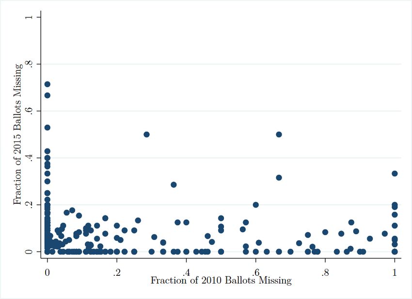
Democracy is an important institution for economic outcomes—both macroeconomic (Acemoglu
et al. 2019) and microeconomic (Kudamatsu 2012, Naidu 2012). Since democracy complements a
market-based economy, a major component of the U.S.’s foreign policy has been democracy assis-
tance (Rose 2000). From 2015 to 2018, expenditures on democracy assistance programs by USAID
and the US State Department averaged $2.2 billion per year (U.S. Government Accountability Of-
fice 2020). These programs support elections, but sometimes they include direct interventions. In
the short-run, such interventions tend to succeed in promoting the US’s preferred candidate (Levin
2016). But interventions might replace the median voter’s preferences with the U.S.’s, and we do
not know whether this has lasting consequences for democracy in the targeted country.
   To investigate the medium-run consequences of foreign interventions in elections, I look at Haiti
in the 2010 and 2015 presidential elections. In 2010, in the aftermath of a devastating earthquake,
Haiti’s election faced serious challenges after the first round. For the first time in Haiti’s history, the
presidential election advanced to a second round run-off. But there was conflict on which candidates
should advance. Three candidates were in contention: Mirlande Manigat, the undisputed first-
round leader; Jude Célestin, the incumbent party’s candidate and second-place finisher; and Michel
Martelly, who took third place by less than one percentage point. The election rules dictated
that the top two finishers, Manigat and Célestin, would advance, but accusations of fraud and a
strong opposition campaign brought the country to a political impasse. To resolve the problem, the
U.S. and the Organization of American States (OAS) pressured the Haitian government to remove
Célestin from the election and advance Martelly, a solution the Haitian government resisted but
ultimately accepted. I examine how the intervention affected turnout in the 2015 presidential
election.
   To identify the causal effect, I exploit that the intervention disproportionately affected Célestin’s
supporters in 2010. Although the intervention discarded votes for every candidate, it implicitly
validated Martelly’s and Manigat’s votes while disregarding the pivotal Célestin voters. Thus,
the analysis measures treatment using Célestin’s 2010 vote share: the intervention disregarded a
greater share of voters in sections where 40% of the vote went to Célestin than where he won 20%.
With this definition of treatment, the empirical strategy uses a modified difference-in-differences
specification, comparing turnout in sections across the two elections.
   The data come from section-level vote tallies in both the 2010 and 2015 elections, and I provide
new evidence on the data’s legitimacy. Some might worry about whether the vote tallies mean
anything because there were allegations of fraud. Although suspcious tally sheets were discarded,

                                                    2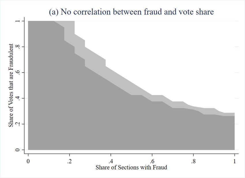
there might be concern that the filtered sheets still contain fraud. To address these concerns, I
match the election results to pre-election surveys and find the results are strongly correlated with
the survey’s predictions. Moreover, tests for vote fraud described in Klimek et al. (2012) report no
significant signs of fraud. Although the test results do not say there was no fraud or that fraud did
not influence the election, they do imply that such irregularities are just noise.
   The modified difference-in-differences results reveal that the U.S. intervention had a strong,
negative effect on turnout. Relative to a section where Célestin won 20% of the 2010 vote, a section
where Célestin won 70% of the vote dropped its 2015 turnout by 3.5 percentage points. The result
is driven entirely by a decrease in votes; there is no difference in voter registration. To support
the results, I run a falsification test using Manigat’s 2010 vote share as the treatment. The same
regression specification shows no effect of Manigat’s 2010 support on 2015 turnout. The results
suggest that the intervention did not discourage Manigat’s pivotal voters, since she remained in
the race, but that removing Célestin adversely affected his pivotal voters.
   Although the data exhibit no strong evidence of fraud, there is still a concern that the noise
might induce a spurious correlation. To address the concerns about fraud, I test the robustness
of the results with two approaches. First, I omit problematic districts identified by the OAS and
find the results persists. Second, I run a sensitivity check to see what patterns of fraud would
create spurious results. Since fraud is unobservable, and there are not even clear indicators on
which sections would be most affected by fraud, the test has to explore different patterns. The
patterns are represented by two parameters: (1) what share of sections experienced fraud and (2)
what percentage of votes in those sections were fraudulent. I run two versions of the test. First, I
assume the intensity of fraud is uncorrelated with Célestin’s vote share. Second, to bias the results
against Célestin, I assume that his top-performing sections are the ones where fraud occurred: if the
assumption is that 10% of sections experienced fraud and that 20% of those votes were fraudulent,
then the simulation removes 20% of Célestin’s votes in sections in his top 10% of support. The
test’s results show that, for the results to be spurious, fraud would have to be much more pervasive
than evidence supports.
   The results warn about the effects of foreign powers intervening in elections. There is some
evidence that foreign aid might improve the integrity of elections (Ubert and Jackson 2020), but
this paper shows that interventions that go beyond financial support could hurt electoral integrity.
Previous work has shown that in the concurrent election, voters in a targeted country tend to
support the candidate promoted by the intervention (Levin 2016). In hypothetical interventions,

                                                  3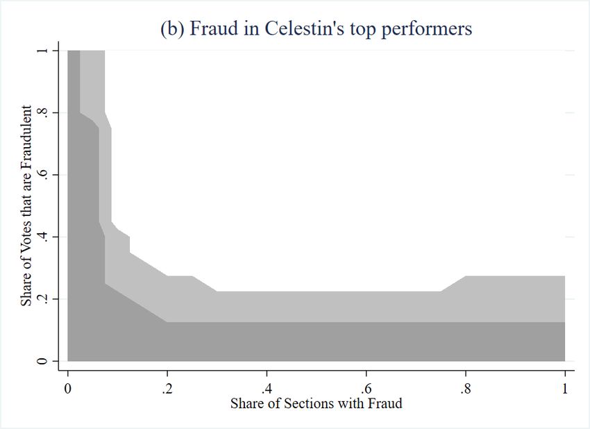
we know that voter support for the intervetions depends on whether the it fits their political
preferences (Corstange and Marinov 2012). But we do not understand how foreign interventions
affect subsequent elections. The extent to which the election is hurt could depend on the strength of
the electoral institutions. For instance, work by Allcott and Gentzkow (2017) suggests that Russia’s
interference in the U.S. 2016 presidential election likely had an inconsequential effect on the results,
and the historic-high turnout in the 2018 midterm elections suggests that any discouragement effect
would have been small too. But since many countries that receive democracy assistance are only
in the initial stages of a political transition, the intervention’s effects could be different. When
weighing the costs and benefits of a democracy assistance intervention, the US should recognize
that short-run benefits could be offset by long-run costs.
   These results also contribute to our understanding of the economics of voting. That canonical
voting model from Downs (1957) posits that voters go to the polls based on the cost of voting,
the benefits of the policy, and the expectation that the voter will swing the decision; later models
include utility from the act of voting (Riker and Ordeshook 1968). With the Downsian model in
mind, there are two ways to think about the results. First, the intervention discarded votes from
pivotal voters, so it may reduce a voter’s subjective beliefs that he will swing the decision. The
importance of beliefs about being a pivotal voter have been debated—lab results show a positive
correlation between beliefs and voting behavior (Duffy and Tavits 2008) and that voters will abstain
from voting if they are uninformed and believe they are pivotal (Battaglini et al. 2010), but data
from small-scale elections suggest that winning margins are too large for the pivotal voter model to
explain voting behavior (Coate et al. 2008). While I cannot conclude that the pivotal-voter model
explains Haitian behavior, one interpretation is that the intervention changed the pivotal voter from
Haitian citizens to foreign actors, diminishing the incentive to vote. A second possible mechanism
is that the intervention decreased the expected utility from voting. Since utility from voting and
performing civic duties strongly influence voter behavior (Dellavigna et al. 2017, Gerber et al. 2008,
Ali and Lin 2013), foreign actors need to be aware that an intervention could significantly affect
how voters enjoy elections.
   Finally, these findings are a significant deviation from similar empirical work on disenfranchise-
ment from fighting fraud. The intervention disenfranchised many Haitian voters by disregarding
their votes due to apparent irregularities. This parallels many debates in the U.S. about policies
that prevent election tampering but that might also disenfranchise voters. For instance, a rising po-
litical issue in the U.S. is the fight over voter identification laws. While some believe that such laws

                                                   4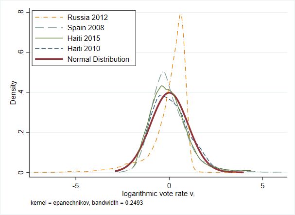
will fight fraud, others believe requiring identification will disenfranchise groups who are less likely
to have government issued IDs. Yet empirical work has shown that such laws have no significant
effects on fraud or on turnout (Cantoni and Pons 2019, Hoekstra and Koppa 2021).1 On the other
hand, voters in Florida were more likely to vote if their right to vote had been threatened by an
aborted state-wide purge (Biggers and Smith 2020). But these studies look at voter behavior in the
U.S., a country with established democratic institutions. Countries with weak or new democratic
institutions, on the other hand, may respond differently to disenfranchisement (Collier and Vicente
2012).

1       Background on Haitian politics, 1990-2016

Haiti has a long history of fraught politics, and foreign intervention is not unfamiliar. The cumu-
lative effect of this history has shaped Haiti’s politics over the past three decades.

1.1      Elections and the International Community, 1990-2006

Ever since democracy started in Haiti in 1990, the international community has been involved
to some degree. The smallest and least controversial role it has played has been to monitor the
elections. Monitoring began in the first election in 1990, when Haiti’s provisional government invited
several hundred international observers to monitor the election, which Jean-Bertrand Aristide won
with 70% of the vote (von Hippel 1995). The first major intervention was in 1995. After a coup
had ousted Aristide in 1991, less than eight months after taking office, the international community
helped return him to the presidency in 1994 on the condition that he step down in 1995 and hold
an election (Mobekk 2001). The nature of the international community’s involvement changed
in the election of 2006 with two major interventions. First, the international community forbade
Aristide’s party (Fanmi Lavalas) from running a candidate (Dupuy 2006). Second, the international
community influenced the vote count. The election committee, when counting the votes, discovered
a significant number of ballots were blank. It was unclear whether the blanks were mistakes, protest
votes, or intentional fraud, but according to election rules they had to be counted. But there were
enough blanks that including them in the total would dilute the leading candidate’s vote share
enough to force a second round. The international community intervened, saying that while the
blanks had to be counted, the rules did not specify how they had to be counted, and awarded them
    1
   Similarly, many states disenfranchise ex-felons, but even before they were convicted of crimes these voters had
some of the lowest turnout rates (Burch 2011).

                                                        5
proportionally to each candidate, thus avoiding a run-off (Dupuy 2006).
With the coups and electoral interventions through the 1990s and 2000s, Haitian voters became
disillusioned with the election process, which led to large variation in turnout. One source of
disillusionment was that people did not see results from the political process. The international
community was so focused on elections that they often ignored the abusive administrations they
created, which eroded trust in the international community (von Hippel 1995). Many Haitians lost
faith in the election process, believing that it never led to change, and they came to refer to their
system as pepe (secondhand) democracy. Accompanying this disillusionment was a decline in voter
turnout. In 1990, 50% of registered voters turned out, but in 1995, when Aristide was forced to step
down despite his interrupted first term, turnout for the election was around 28% (Nohlen 2005 p.
392). The turnout for the legislative election in 1997 was even lower at 5 percent (Mobekk 2001).
Controversy over the first round of the 2000 election was followed by low turnout in the second
round. But by 2006 turnout swelled to 63% (Dupuy 2006 pp. 168-169).
While the international community has meddled with Haitian elections, we do not know whether
its influence has caused Haitians to change their voting behavior. One difficulty with attributing
any adverse effects is that the interventions were often small. For instance, although one of the
conditions for restoring Aristide was that he allow the election to proceed as scheduled in 1995 and
to not run as a candidate, the condition was enforcing constitutional restraints. Haitian presidents
cannot serve two consecutive terms. The controversy was whether Aristide’s interrupted tenure
counted as a full term. Similary, the 2006 interventions did not seem to alter the outcomes of the
election. While the international community prevented Aristide’s party from officially running a
candidate, the party’s 1995 candidate and winner Rene Préval created a new party and won in
2006. While Préval’s victory was helped by the intervention that pushed his first-round vote share
above 50%, he was the clear favorite leading up to the election, with the runner-up only receiving
12% (Dupuy 2006). Thus, while the international community intervened, its actions were arguably
inconsequential. But that changed significantly with the 2010 election.
1.2 The 2010 Presidential Election
In November 2010, 10 months after an earthquake that killed 200,000 people, Haiti held a pres-
idential election. Turnout was low at 23%, which was to be expected because of the tumultous
post-earthquake environment. But that was not the only problem with the election; the OAS,
whom the Government of Haiti had invited to monitor the election, reported, “the day of elec-
6tions was marred by disorganization, dysfunction, various types of irregularities, ballot stuffing and
incidents of intimidation, vandalism of polling stations and violence” (Organization of American
States 2011b). While acknowledging the problems, the OAS expressed confidence in the election:
“Based on its observations in the eleven electoral departments, the Joint Mission does not believe
that these irregularities, serious as they were, necessarily invalidated the process” (Organization
of American States 2010). Despite this supporting statement, counting the votes was contentious.
The Provisional Electoral Council (CEP) failed to receive 1,365 tally sheets (about 12.2% of the
vote). Then, before reporting the results, the Provisional Electoral Council (CEP) discarded 312
tally sheets (about 7.6% of votes) that appeared “irregular” (Johnston and Weisbrot 2011).
With a first round that had 18 candidates, no candidate won a sufficient share of the votes to
become the outright winner. Haitian elections consist of a first round of voting with all candidates,
but if no candidate wins more than 50% of votes then a second round run-off is held with the
top two candidates. After counting the remaining votes, the leading candidate, with 31.4% of the
vote, was Mirlande Manigat, a university administrator and former First Lady. In second place,
with 22.5%, was Jude Célestin, the candidate hand-picked by then-president Rene Préval. Finally,
in third place, with 21.8% of the vote (less than 1 percentage point behind second), was Michel
Martelly, a music star on his first political foray. For the first time in Haiti’s history, the presidential
election would require a run-off.
Despite the CEP’s removal of “irregular” tally sheets, some accused Célestin of using Préval’s
administration to manipulate the election, and the election results were protested. The OAS
expressed little faith in the claims, “More subversive of the process was the toxic atmosphere
created by the allegations of ’massive fraud’. The [election monitors] observed instances where even
before the voting started, any inconvenience or small problem led to the immediate cry of fraud”
(Organization of American States 2011b). Indeed, the claims were so tenuous that while Manigat
and Martelly initially led the charge for canceling the vote, they withdrew their complaints once
they heard they were in contention for the run-off (Katz 2013 p. 255). A week after the election, the
Government of Haiti requested that the Organization of American States (OAS) review the tally
sheets and verify the results (Organization of American States 2011a p. 24). After its investigation,
the OAS recommended that the CEP discard another 234 tally sheets consisting of nearly 51,000
votes (4.7% of the counted votes). Discarding these sheets would put Célestin in third place and
move Martelly into the second round against Manigat.
But the government of Haiti initially refused to implement the recommendation. The refusal
7created weeks of a political stalemate. Finally, U.S. Secretary of State Hillary Clinton visited Haiti
on January 30, 2011 and told President Préval the OAS recommendations would be implemented
(Katz 2013, p. 270). The evening of Clinton’s appearance, the government announced the final
round of the election would be between a former First Lady (Manigat) and a celebrity with no
political experience (Martelly). The second round was held on March 20, 2011. Despite removing
Célestin from the election, there were similar problems in the second round, and 15.3% of tally
sheets were discarded for irregular counts (Organization of American States 2011a p. 28). On May
15, Michel Martelly became president.
The Martelly administration did not improve confidence in democratic institutions. During
Martelly’s five-year term, the country failed to hold an election at any level of government, and
by 2015 the majority of legislators’ terms had expired, leaving the president to rule by decree.
Despite difficulties, presidential elections were held in October 2015. Since the constitution prohibits
presidents from serving consecutive terms, Martelly could not run again. Instead, he picked Jovenel
Moïse, a banana farmer with no political experience, as the candidate for his party. Although 54
candidates ran, the principal contender was again Jude Célestin.
The 2015 election had similar problems as 2010. After the first round, there were many reports
of fraud and misconduct. A commonly cited problem was the the election monitors.2 The monitors
were representatives from each political party and were stationed at each polling location. While
the logic for the monitors was that they would prevent each other from cheating, instead it was
widely reported that smaller parties were selling their monitors to larger parties. The problems
with the 2015 election were so large that no one would allow the elections to advance to the second
round, and in February 2016 President Martelly resigned and a provisional president took his place.
Uncertainty about the next election persisted through 2016. The provisional president’s man-
date ended in June, without a clear plan on when the election would be held. Then in October,
Hurricane Matthew disrupted the country, killing many. Finally, after a year of uncertainty, an-
other first-round presidential election was held in November 2016. Many of the candidates from
the 2015 election had dropped, halving from 54 to 27, and Jovenel Moïse, Martelly’s hand-picked
successor, won the election outright. Although accusations of fraud were minimal, there was a
significant concern that participation was low, with only 18% voter turnout.
Did the events of 2010 affect the 2015/2016 elections? Although a causal connection has yet to
2
For more information on the controversy, see the summary by Jake Johnston at the Center for Economic
and Policy Research, available at https://web.archive.org/web/20190809152541/http://cepr.net/blogs/haiti-relief-
and-reconstruction-watch/presidential-elections-in-haiti-the-most-votes-money-can-buy.
8be established, there is evidence that confidence in the democratic process had faltered. Between
the 2015 and 2016 round of voting, Kolbe and Muggah (2016) surveyed over 2,000 households about
their feelings towards the election. The overwhelming favorite candidate among these households
was Célestin, receiving support from 42% of respondents, and Moïse was the least preferred can-
didate at 4%. But only 16% of households said they had voted in the 2015 election, and only 3%
said they would vote in the rerun of the first round in 2016. While the report does not report
cross-tabulations of candidate preference and participation, it is clear that Célestin voters were not
participating. The most popular response for non-participation was concern over fraud or lacking
confidence that the vote would be counted (26% gave it as their main reason) and the second most
popular response was that there was no point in voting (19%). The voters did not rationalize their
responses, but when asked about hypothetical solutions to the 2015/2016 electoral crisis, some of
the least popular options involved interventions by foreign states or organizations. Thus, while
none of this evidence is strong enough for a causal connection between the intervention in 2010 and
the low turnout in 2015/2016, there is certainly enough circumstantial evidence to suggest further
investigation of whether Célestin’s supporters lost faith in the democratic process.
2 Identifying the effect of disenfranchisement on turnout
Although it was a political travesty, several aspects of the 2010 presidential election provide a conve-
nient environment for testing whether foreign intervention hurt democratic institutions. According
to Shulman and Bloom (2012), foreign interventions in elections are most likely to trigger pushback
when they are salient, partisan, and directed by the state rather than a non-state actor. Haiti in
2010 met all of these conditions: the intervention was ultimately effected by the US Secretary of
State (state actor) in an openly acknowledged process (salient) that excluded a particular candidate
(partisan).
In addition to meeting the theoretical conditions, there are other reasons why this election
is appropriate for this question. First, even though Haitian elections have a history of foreign
influence, this intervention was more explicit than previous elections. A good contrast for the
2010 intervention was the previous election’s intervention. In 2006, the international community
assured a quick victory for Préval by exploiting a legal ambiguity about counting blank votes.
The intervention was subtle and could easily go unnoticed. In 2010-11, however, the international
community had delayed the second round for months calling for Célestin’s removal, which finally
happened the same day as a high-profile visit from the U.S. Secretary of State. Second, the
9intervention unambiguously changed who became president. Again, 2006 is a good contrast. While
assuring Préval’s victory required a slight push, he was the clear favorite and no one was surprised
by the outcome. In 2011, however, removing Célestin allowed Martelly to advance against Manigat.
If Manigat had won, one could always debate whether the intervention affected the outcome. But
Martelly won, which would not have been possible without the intervention.
A second convenience is that the intervention discarded legitimate votes. While the intervention
was rationalized as a way to remove fraud from the election, the implementation was crude. If a
tally sheet was deemed “irregular,” every vote on the tally sheet was discarded. Rosnick (2010)
gives a simple example of the harm this could cause: suppose the true votes on a tally sheet are 120
for Célestin and 50 for Manigat, but that the sheet reads 180 for Célestin and 50 for Manigat. The
extra 60 votes are fraudulent. While a true correction would eliminate those 60 votes and properly
represent the section’s preferences, discarding the entire tally sheet trades an error of +60 votes for
Célestin for a net error of +70 votes for Manigat, which is a 130 vote swing in that section. Rosnick
then uses a simulation of the discarded tally sheets to show that Célestin’s legitimate votes likely
gave him an indisputable lead over Martelly. The intervention not only directly disenfranchised
voters by discarding their votes, it indirectly disenfranchised all voters who had voted for Celesin.
Another convenience of this setting is that Célestin ran in both elections. Having Célestin in
both elections is nice because it keeps the personality constant. Personality drives Haitian politics
because there are no stable political coalitions that attract consistent support. In each election,
dozens of candidates ran for president across just as many parties, and between elections Célestin
even switched political parties. Having Célestin, the target of 2010’s intervention, run in both
elections means that we can control for the personality and be more confident that the effects are
driven by the intervention.
Predicting how the intervention affected the subsequent election is difficult because the rela-
tionship between disenfranchisement and turnout is theoretically ambiguous. According to reactive
theory, disenfranchisement may cause voters to cherish their voting rights, increasing turnout in the
next election (Biggers and Smith 2020). For instance, when the Voting Rights Act of 1965 reversed
the disenfranchisement of Blacks in the South, Black voters registered to vote and turned out in
high numbers (Cascio and Washington 2014). On the other hand, the intervention could discour-
age Célestin’s supporters, fracturing their fragile faith in the democratic system. Such voters may
question the purpose of participating in the election, especially when inefficient polling stations and
dangerous election-day conditions significantly increase the cost of voting. In this case, we would
10observe a decrease in turnout.
To estimate how the intervention affected voter behavior, I examine turnout across the two
elections using Célestin’s vote share to measure intensity of treatment. I use a modified difference-
in-differences strategy similar to Jones et al. (2017) and estimate the following regression:
yst = β1 Disenf ranchisements × P ostInterf erencet + δt + δs + β2 Xst + εst . (1)
The dependent variable yst includes election outcomes such as turnout or registered voters in
section s in election t ∈ {2010, 2015, 2016}. Disenf ranchisements measures the degree of disen-
franchisement in secions s, which I proxy with Célestin’s 2010 vote share. The dummy variable
P ostInterf erencet indicates whether it is the 2015 or 2016 election. The regression includes election
and section fixed effects (δt and δs , respectively) and controls for the cholera rate (Xst ), explained
below.
Identifying a causal effect from the intervention rests on the assumption that Célestin’s 2010
vote share did not affect changes in turnout within a section across elections except through the
response to the intervention. One way to frame the identifying assumption is to say that in a
world where Célestin was not dismissed from the 2010 election we do not expect turnout to change
differently within a section that voted 40% in favor of Célestin than in a section where only 10%
of voters supported him. Of course, a section that voted 10% for Célestin must have given more of
its votes to another candidate, so another way to frame the identifying assumption is to say we do
not expect turnout to change differently within a section that voted 40% in favor of Célestin than
in a section where 40% voted in favor of Manigat or Martelly.
One assumption embedded in this analysis is that the voters who were disenfranchised in 2010-11
were still in their sections in 2015-16. If voters move to other sections but retain the consequences of
their response to the intervention, then the effects will spillover into other sections. Unfortunately,
we do not know whether migration is a problem or not. Haiti’s last census was in 2003 and there
are no regular surveys of migration. Nevertheless, the effect on the analysis should be minor. As
long as the migration destination is orthogonal to the Célestin’s 2010 vote share in the origin, this
means there is error in measuring the treatment status, which biases the estimates of β1 towards
zero.
112.1 Fraud as a threat
Another threat to the analysis is fraud. Even though the OAS expressed confidence in the election,
there is still concern that there is fraud present in the data. Most importantly, if fraud in 2010 was
correlated with Célestin’s vote share—an easy case to make since he was removed on suspicion’s of
fraud—and if that fraud was eliminated in 2015—also reasonable since his party was no longer in
power—then the analysis would produce a negative coefficient.
One protection against fraud in the analysis is that the CEP reportedly eliminated the most
egregious examples of fraud. The intervention’s purpose was to secure the integrity of the election,
which the CEP did by getting rid of tally sheets that looked “irregular.” The remaining sheets,
which are the only ones used in this analysis, passed the CEP’s scrutiny. Thus, while we cannot
guarantee the remaining ballots are free of fraud, the fraud was noisy enough to avoid detection.
An important point to note is that while Célestin was under the most scrutiny, there was no
definitive evidence that he cheated nor evidence that the other candidates did not cheat. The
OAS reports never attribute fraud to any party nor exempt any parties from fraud. In fact, as
mentioned above, more “irregular” sheets were discarded in the second round, when it was only
Manigat and Martelly, than were discarded in the first. Thus, while fraud may exist, it is possible
that all candidates received fraudulent votes.
Unfortunately, it is impossible to resolve the problem of fraud in the analysis. Nevertheless,
I take three approaches to address it. First, I examine the data for patterns of fraud using tests
described in Klimek et al. (2012). The analysis in Section 3 shows that Haiti’s elections exhibit
patterns consistent with unbiased elections. Note that the finding that there is no strong pattern
of fraud is not surprising given the CEP examined the 2010 ballots and invalidated suspicious ones
(the analysis is performed on the filtered results). Some question the process CEP used to identify
suspicious ballots (Johnston and Weisbrot 2011), but it seems the ballots that remained do not
present a strong case for fraud. We cannot rule out that there was no fraud in the election, but it
looks like the main concern is that it creates a noisy measure of turnout and true vote shares. In
that case, the specification in Equation 1 would treat fraud as part of the error term, εst , and as
long as it is unrelated to Célestin’s 2010 vote share, the estimate would be unbiased.
The second and third approaches rely on observations from the OAS election monitoring re-
port. The second approach assumes that the OAS report accurately identified that the problems
with fraud were concentrated in Port-au-Prince and that the provinces’ problems were not with
fraudulent voting. Under this assumption, the easy test for the results’ robustness is to remove
12observartions from Port-au-Prince and the surrounding areas.3 The third approach uses the OAS
observations to design a sensitivity test. The report claims the problems were concentrated in a few
areas. The question is, how many sections experienced problems? And for such sections, how many
of Célestin’s votes were fraudulent? These questions establish a clear foundation for a sensitivity
test that examines how robust the results are to perturbations in the data.
3 Data on Haitian elections
Election data in Haiti are scarce, but in this case we have enough data to at least investigate
the question. The data come from election results in the first round of the Haitian presidential
elections in 2010 and 2015 and the repeat first-round election in 2016. Ahead of the presidential
elections, there were concerns about preventing fraud and creating a legitimate election. To assuage
concerns, the CEP posted vote tallies for each polling station in the country. The 2010 vote tallies,
without the 312 sheets discarded by the CEP, were collected by Johnston and Weisbrot (2011), and
I collected the 2015 and 2016 data directly from the CEP tallies.
Unfortunately, there are no publicly available disaggregated data for the second round of 2010
(the runoff between Manigat and Martelly) or for any election before 2010. On the one hand, the
absence of data prevents me from exploring the validity of the parallel trends assumption. On the
other hand, investigating how foreign interventions affect political participation almost by definition
occurs in countries with scarce data. Governments that regularly track election data and make the
disaggregated results publicly available have stronger electoral institutions and therefore are not a
target for foreign intervention.
The vote tallies allow us to measure turnout in both elections and Célestin’s vote share in 2010.
Calculating turnout is challenging because we do not have the exact number of registered voters in
each section. But we can proxy for the number of registered voters using the number of booths in
each section because booths were assigned to sections according to the number of registered voters:
one booth for every 550 registered voters. In 2010, the average section had about 16 booths, and
by 2015 the average section had 19 booths, which reflects that voter registration increased between
the two elections. Since booths are determined by the number of registered voters, for a section
with N booths, we know there are at least (N − 1) × 550 registered voters. The complication is
in the last booth, which could represent anywhere between 1 to 550 voters. Because the data do
3
Specifically, the following districts are omitted: Port-au-Prince, Carrefour, Cite Soleil, Delmas, Gressier, Kenscoff,
Petionville, and Tabarre.
13Table 1: Summary Statistics on election turnout and Célestin’s vote share
All Sections Bottom Quartile Top Quartile Difference
A. Turnout
Célestin 2010 Vote Share 0.26
[0.17]
Turnout 2010 0.26 0.23 0.29 0.06***
[0.10] [0.10] [0.11] [0.012]
Turnout 2015 0.26 0.25 0.27 0.02***
[0.07] [0.07] [0.07] [0.0081]
Turnout 2016 0.19 0.18 0.20 0.02**
[0.08] [0.08] [0.08] [0.0087]
N 612 153 153
B. Section Characteristics (2009)
School - Elementary 0.95 0.97 0.94 -0.030
[0.21] [0.18] [0.25] [0.028]
School - Secondary 0.51 0.62 0.34 -0.28***
[0.50] [0.49] [0.47] [0.062]
School - Technical 0.15 0.30 0.06 -0.24***
[0.36] [0.46] [0.25] [0.047]
Post Office 0.03 0.05 0.01 -0.044**
[0.16] [0.22] [0.09] [0.022]
Court 0.10 0.13 0.07 -0.057
[0.29] [0.34] [0.26] [0.039]
Internet Cafe 0.15 0.32 0.08 -0.24***
[0.36] [0.47] [0.27] [0.049]
Cell Coverage - Total 0.19 0.23 0.15 -0.081
[0.39] [0.42] [0.36] [0.051]
Cell Coverage - Partial 0.64 0.66 0.58 -0.088
[0.48] [0.47] [0.50] [0.063]
Pharmacy 0.24 0.39 0.12 -0.27***
[0.43] [0.49] [0.33] [0.053]
Sanitation 0.45 0.57 0.28 -0.29***
[0.50] [0.50] [0.45] [0.061]
Gas Station 0.08 0.20 0.02 -0.17***
[0.27] [0.40] [0.15] [0.039]
Recreation 0.13 0.22 0.07 -0.14***
[0.34] [0.41] [0.26] [0.044]
N 483 116 125
Notes: The columns with “quartile” in the heading refer to the quartiles of Célestin’s 2010 vote
share. The bottom quartile is sections where Célestin won less than 12.5% of the vote, and the
top quartile includes sections where he won more than 35.5%. In the Difference column, standard
errors are in brackets, for all other columns standard deviations are in brackets. *** pnot allow me to identify the marginal booth, I assume all booths have 550 registered voters. This
assumption’s robustness is explored in the appendix.
Summary statistics for turnout and Célestin’s vote share are reported in Table 1. In 2010,
Célestin’s average vote share was 26%; average turnout was also 26%. While the 2010 turnout
should have been depressed by the post-earthquake recovery environment, the average turnout
across sections remained constant in 2015 at 26%. But average turnout in 2016 dropped to 19%,
widely attributed to voter fatigue after a year of uncertainty about elections. Since the empirical
strategy measures disenfranchisement through Célestin’s vote share, it is helpful to split the data by
Célestin’s vote share, comparing the top quartile of his support with the bottom. In each election,
Célestin’s top quartile of 2010 sections had higher (statistically significant) turnout than the bottom
quartile. Across elections, turnout changed differentially by quartile of Célestin support. From 2010
to 2015, we see that sections in the bottom quartile increased their turnout (23% to 25%) but that
the top quartile’s turnout declined (29% to 27%). In 2016, turnout had declined relative to 2010,
but in the bottom quartile it had dropped only 5 percentage points, whereas in the top quartile it
declined by 9. Thus, there is evidence that voter behavior responded differently across elections,
though the mechanism behind the difference is yet unclear.
We can look at which sections supported Célestin using a 2009 amenities census. In 2009, the
Ministry of Agriculture (MARNDR) surveyed sections to assess the amenities available around the
country. Such amenities include the types of school available (elementary, secondary, and technical),
the presence of state services (post office and court), access to information technology (presence
of internet cafe and cell phone coverage), and other amenities (sanitation facilities, gas station,
and recreation center). Table 1 shows that of the 12 amenities measured, sections in Célestin’s
top quartile of support were less likely to have every one than the sections in the bottom quartile,
with 8 of the 12 differences being statisically signficant at the 5% level or stronger. This strongly
suggests that Célestin’s support came from poorer voters. This is unsurprisiing since Célestin was
running under the Unity party, whose founder was then-president Rene Préval, who owed his 2006
victory to large turnout in poor areas (Dupuy 2006 p. 169).
Since there is a clear difference in the characteristics of sections that supported Célestin in 2010,
we need to pause and address how this will affect the analysis. Ideally, the analysis would account
for the initial differences and control for changes over the five years. But this is Haiti, a country
where data are scarce. While Haiti has a national statistics office, before the earthquake it did not
regularly collect data, and it certainly did not collect much data in the chaotic period following the
15earthquake. Even accounting for population changes is difficult because the population projections
were based on assumptions of constant population growth (see the appendix). Thus, the analysis
cannot account for changes in section characteristics over time. Nevertheless, Haiti was not a
dynamic economy. Of course it experienced a significant shock with the 2010 earthquake, but this
survey measured amenities in 2009, so the differences in characteristics predated the earthquake.
After the earthquake, Haiti’s economy stagnated, with GDP per capita growing an average of 0.5%
per year (in contrast with the Dominican Republic, its island neighbor, which during the same
year grew 4.2% per year). Thus, while the analysis cannot control for how sections changed in
the years between the elections, there is not a strong argument that section characteristics were
changing enough to even warrant a concern. Controlling for initial differences using section fixed
effects should be sufficient.
There was one section characteristic, however, that changed during this period, and probably in-
fluenced the election: the cholera rate. After the earthquake, cholera was introduced to the country
by Nepalese UN workers (Katz 2013, Ch. 11). Because of Haiti’s poor sanitation infrastructure,
the cholera spread through the country, but it of course had differential effects. Controlling for
cholera is important because it evolved into a contentious political issue and could spark an elec-
toral response. Thus, all regressions control for the district’s cholera rate (note: districts are made
of several sections).
3.1 Does voter fraud affect the analysis?
Because voter fraud was a central issue in the aftermath of both the 2010 and 2015 elections, it
is important to establish the extent to which such fraud may confound the analysis. There are
two factors under consideration. First, many ballots were missing or not included in the vote
tallies—how should such cases be handled? Second, if fraud is such a large issue, do the election
results have any meaning?
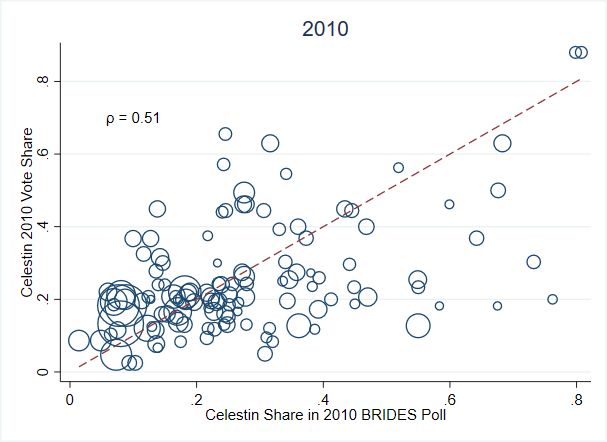
Resolving the concern about missing ballots is straightforward. The CEP reports how many
ballots were missing or discarded in each election, and both elections had problems—in both 2010
and 2015, 30% of sections had at least one missing ballot. Although in both elections the percentage
was equal, it was uncommon for the same section to have missing ballots in both years, as seen
in Figure A1. If a ballot is missing, we can still estimate turnout and Célestin’s 2010 vote share
from the other ballots in the section. But missing ballots decrease our confidence in the measure’s
accuracy. To address the concern, regressions are weighted by the fraction of ballots recovered—we
16weight an observation more if we have 100% of its ballots than if we have only 50%. For robustness,
unweighted results are reported in the appendix.
The concern about whether the fraud destroys any meaning behind the results is more difficult.
We have at least some confidence that the data have minimal fraud since the election authorities
discarded 546 tally sheets that looked irregular. Although we cannot say that all fraud is eliminated
(or even if the discarded sheets contained fraud) the data should have few cases of extreme fraud.
But just because the allegedly extreme cases have been eliminated does not mean there is no fraud
it what remains. Unfortunately, it is impossible to identify election fraud relying on just election
results; however, it is possible to analyze such results and see if the patterns match those predicted
by models of election fraud. In what follows, I present evidence from pre-election surveys and
election patterns to argue that nothing in the data suggests fraud confounds the analysis. But let
me be precise about how to interpret the analysis: I am making an argument about fraud’s effect
on the analysis, not its effect on democracy. Fraud was clearly an issue in the elections, and such
concerns should be taken seriously because they affect the election’s integrity. My argument is that
to the extent which it did occur, fraud did not significantly skew the data and can be interpreted
as noise, obscuring the precision but not the estimates. This is consistent with the ballots passing
the CEP’s inspection, as described above.
Evidence from pre-election surveys suggests voting results reflected the district’s preferences. In
both 2010 and 2015, pre-election polling was conducted by the Bureau de Recherche en Informatique
et en Developpement Economique et Social (BRIDES) at the district-level (which is one step of
geographical aggregation above sections). The BRIDES survey is the only source of data outside
of election results that measures local political preferences, but it is not perfect. Although the
BRIDES survey allegedly followed sound survey practices, it is clear from the demographic data
presented in Table A1 that the respondents do not represent the country’s population (though, in
defense of BRIDES, it might be a fair representation of the people who voted). Furthermore, the
sample size is small: in 2010, the average number of respondents per district was 57, and in 2015
it was about 100, leaving significant room for sampling error. Nevertheless, if we want to validate
the election results with an outside source, the BRIDES survey is the only benchmark available.
Despite the survey’s weaknesses, the district-level results correspond favorably to the election
results. Figure 1 shows scatter plots of the election results against the survey results for both
2010 and 2015, and there is a clear relationship between them. The correlation is stronger in
2015 (ρ = 0.76) than in 2010 (ρ = 0.51), but this is expected with the difference in sample sizes.
17Figure 1: Relationship between pre-election polls and 2010/2015 election results by district
Notes: Data come from pre-election surveys conducted by Bureau de Recherche en Informatique
et en Developpement Economique et Social (BRIDES) in October of the election year. Each dot
represents a district. The 2010 plot weights districts according to sample size, but in 2015 the
sample size was the same for every district. The top-left corner of each plot reports the correlation
coefficient (ρ).
18Although there is room to question the independent validity of the BRIDES survey and the election
results, their strong correlation suggests that the election results reflect the district’s preferences.
While that test used external data to validate patterns in the results, another test looks for
fraud indicators just using patterns in the election data. One visual test looks at how many voting
booths had unusually high turnout and unusually high support for the winner. Klimek et al. (2012)
call this the election thumbprint. The intuition is simple: if someone illegally adds 100 votes for
a candidate, that will increase the candidate’s vote share, but it will also increase the measured
turnout because it looks like 100 more voters participated. Thus, sections with both anomalously
high turnout and high support for the winner are likely locations of ballot stuffing. Indeed, one
criterion for examining tally sheets for irregular voting patterns was whether the sheet had over
50% turnout (Organization of American States 2011a p. 98).
The simplest way to implement this test is to plot the suspicious party’s vote share against
turnout, as shown in Figure 2. This figure plots the thumbprint for four presidential elections:
Haiti’s 2010 and 2015, Spain’s 2008, and Russia’s 2012. In Russia’s 2012 election, practically no
booths fell into the lower triangle of low turnout and low support, but there is a distinct smear to
the northeast corner of the scatter plot. Klimek et al. (2012) conclude that the smear is compelling
evidence of fraud in Russia’s election as ballot stuffers pushed up both Putin’s share and the
observed turnout. Spain, on the other hand, is shown as an example of a thumbprint that displays
no indication of fraud: turnout is high, but there are few booths in the upper triangle of both
high turnout and high support for the winner. For Haiti, the two thumbprints appear much more
like Spain than Russia, with no booths reporting high turnout. Even conditional on low turnout
numbers, very few booths report high support for Célestin.
The data do not raise any red flags for fraud and are suitable for analysis. The findings are
consistent with the CEP filtering suspicious ballots and presenting only the results it trusted. As
mentioned above, the analysis cannot unconditionally reject the presence of fraud or determine the
effect of fraud on the election results. Furthermore, the analysis cannot reject interventions with
marginal impacts on vote counts, such as vote buying or voter intimidation. But the data appear
to accurately reflect district preferences, and fraud might add some noise to those measures. In
a regression analysis, any fraud is treated as measurement error. The sensitivity test will address
how such measurement error affects the robustness of the results.
19Figure 2: Election fingerprints for presidential elections in Spain (2008), Russia (2012), and Haiti (2010, 2015)
20
Notes: Election fingerprints let you see if any sections had unusually high turnout and unusually high support for the winner. Russia is
an example where booths with high turnout also often had a high share of votes going to Putin, evidence that ballot stuffing influenced
the election. Dots represent cells of turnout and vote share, and dots are weighted by the number of sections in each cell. Data for Spain
and Russia come from Klimek et al. (2012).Table 2: The effect of the disenfranchisement in 2010 on turnout in Haiti’s 2015 and 2016 presi-
dential elections
Turnout ln(Turnout) ln(Registered) ln(Votes)
Célestin Share in 2010 ×Post Interference -0.069*** -0.31*** -0.073 -0.38***
[0.018] [0.078] [0.057] [0.099]
2015 Election -0.0099 0.013 0.16*** 0.18***
[0.0084] [0.035] [0.028] [0.046]
2016 Election -0.074*** -0.31*** -0.056* -0.37***
[0.0087] [0.037] [0.029] [0.049]
sinh−1 (Cholera Rate) × 2015 Election 0.0075*** 0.026*** 0.0038 0.030***
[0.0015] [0.0061] [0.0050] [0.0080]
R-squared 0.305 0.339 0.245 0.452
Notes: All regressions have three years of data on 614 sections. Standard errors are clustered at
the section level. Because the votes on missing ballots have to be imputed, regressions are weighted
by the fraction of the section’s ballots recovered. *** pTable 3: The effect of the disenfranchisement in 2010 on turnout in Haiti’s 2015 and 2016 presi-
dential elections, disaggregated
Turnout ln(Turnout) ln(Registered) ln(Votes)
2015 Election
Célestin Share in 2010 ×2015 Election -0.063*** -0.30*** -0.067 -0.37***
[0.019] [0.077] [0.066] [0.11]
2015 Election 0.002 0.049 0.15*** 0.20***
[0.0089] [0.035] [0.032] [0.048]
sinh−1 (Cholera Rate) × 2015 Election 0.0045*** 0.018*** 0.0058 0.023***
[0.0016] [0.0059] [0.0056] [0.0083]
R-squared 0.032 0.059 0.281 0.236
2016 Election
Célestin Share in 2010 ×2016 Election -0.075*** -0.32*** -0.081 -0.40***
[0.021] [0.099] [0.069] [0.12]
2016 Election -0.085*** -0.35*** -0.045 -0.39***
[0.010] [0.047] [0.033] [0.057]
sinh−1 (Cholera Rate) × 2016 Election 0.010*** 0.035*** 0.0019 0.037***
[0.0018] [0.0081] [0.0058] [0.0098]
R-squared 0.335 0.330 0.034 0.322
Notes: All regressions have three years of data on 614 sections. Standard errors are clustered at
the section level. Because the votes on missing ballots have to be imputed, regressions are weighted
by the fraction of the section’s ballots recovered. *** pTable 4: Testing for mean reversion using Manigat as a treatment
Turnout ln(Turnout) ln(Registered) ln(Votes)
Manigat Share in 2010 ×Post Interference 0.0065 -0.058 -0.031 -0.089
[0.016] [0.065] [0.047] [0.080]
2015 Election -0.028*** -0.043 0.16*** 0.11**
[0.0088] [0.034] [0.028] [0.047]
2016 Election -0.092*** -0.37*** -0.064** -0.43***
[0.0087] [0.035] [0.028] [0.046]
sinh−1 (Cholera Rate) × 2015 Election 0.0071*** 0.025*** 0.0037 0.029***
[0.0016] [0.0061] [0.0050] [0.0081]
R-squared 0.345 0.38 0.201 0.445
Notes: All regressions have three years of data on 614 sections. Standard errors are clustered at
the section level. Because the votes on missing ballots have to be imputed, regressions give more
weight to sections with fewer missing ballots. *** pTable 5: Testing the robustness of the results to dropping Port-au-Prince and surrounding areas.
Turnout ln(Turnout) ln(Registered) ln(Votes)
Célestin Share in 2010 ×Post Interference -0.060*** -0.23*** -0.063 -0.29***
[0.018] [0.075] [0.059] [0.095]
2015 Election -0.012 -0.01 0.16*** 0.15***
[0.0084] [0.034] [0.028] [0.045]
2016 Election -0.076*** -0.33*** -0.065** -0.39***
[0.0087] [0.036] [0.029] [0.048]
sinh−1 (Cholera Rate) × 2015 Election 0.0072*** 0.025*** 0.0056 0.030***
[0.0016] [0.0060] [0.0050] [0.0079]
R-squared 0.354 0.399 0.211 0.465
Notes: All regressions have three years of data on 581 sections. The following districts are omit-
ted: Port-au-Prince, Carrefour, Cite Soleil, Delmas, Gressier, Kenscoff, Petionville, and Tabarre.
Standard errors are clustered at the section level. Because the votes on missing ballots have to be
imputed, regressions give more weight to sections with fewer missing ballots. *** pCite Soleil, Delmas, Gressier, Kenscoff, Petionville, and Tabarre. Table 5, shows the results are
nearly identical and are robust to dropping those districts.
5.2 Sensitivity Check
The second test is a sensitivity check to see how robust the results are to perturbations in the data.
The goal is to see how much fraud would have to have existed in the 2010 election for the decrease
in turnout to come from eliminating fraud rather than from voters discouraged from participating.
The main advantage of this test is to be as transparent as possible about the conditions needed to
believe the results.
The sensitivity test begins with a thought exercise. Suppose that the only fraud left in the
filtered data (i.e. after the CEP removed irregular tally sheets) is one section where 50% of Célestin’s
2010 votes were fraudulent. Would eliminating that fraud be enough to overturn the results? The
results so far suggest that even if one section had egregious fraud, the overall pattern that turnout
decreased among Célestin voters would survive. But what if 50% of Célestin’s 2010 votes in every
section were fraudulent? Eliminating that much fraud in the next election would be good for
democracy but it could also look like turnout had decreased. So the question is: under what
patterns of fraud do the results still hold?
The sensitivity test is designed to answer this question. It has two parameters: (1) the share
of sections in 2010 with fraud and (2) the share of Célestin’s votes that were fraudulent. The
test then runs rounds for every combination of the two parameters between 0 and 1, at intervals
of 5 percentage points. For instance, the test has one round where 10% of sections experienced
fraud, and in those sections 5% of Célestin’s votes were fraudulent. In each round, the test has
four steps. First, the sections with fraud are selected. Since we do not know which sections had
fraud, I perform the test twice with different assumptions about the ballot-stuffing strategy. One
strategy is to stuff ballots in areas where Célestin is weak. Under this strategy, the vote share
in these sections would look closer to section’s with strong support, and therefore there would be
no correlation between fraud and vote share. Thus, the first test assumes no correlation between
fraud and Célestin’s 2010 share. If the round says 10% of sections experienced fraud, then 10% of
sections are selected at random. But another strategy is to target sections that already support
the candidate, which would induce a positive correlation between fraud and vote share. Thus, the
second test assumes a perfect correlation between fraud and Célestin’s vote share. If the round
assumes 10% of sections experienced fraud, the assumption is that it is the sections at the top 10%
25You can also read