The physics of streamer discharge phenomena
←
→
Page content transcription
If your browser does not render page correctly, please read the page content below
The physics of streamer discharge phenomena
arXiv:2005.14588v1 [physics.plasm-ph] 29 May 2020

                                                               Sander Nijdam1 , Jannis Teunissen2,3 and Ute Ebert1,2
                                                               1
                                                                 Eindhoven University of Technology, Dept. Applied Physics
                                                               P.O. Box 513, 5600 MB Eindhoven, The Netherlands
                                                               2
                                                                 Centrum Wiskunde & Informatica (CWI), Amsterdam, The Netherlands
                                                               3
                                                                 KU Leuven, Centre for Mathematical Plasma-astrophysics, Leuven, Belgium
                                                               E-mail: s.nijdam@tue.nl

                                                               Abstract.
                                                                   In this review we describe a transient type of gas discharge which is commonly called
                                                               a streamer discharge, as well as a few related phenomena in pulsed discharges. Streamers
                                                               are propagating ionization fronts with self-organized field enhancement at their tips that can
                                                               appear in gases at (or close to) atmospheric pressure. They are the precursors of other
                                                               discharges like sparks and lightning, but they also occur in for example corona reactors or
                                                               plasma jets which are used for a variety of plasma chemical purposes. When enough space is
                                                               available, streamers can also form at much lower pressures, like in the case of sprite discharges
                                                               high up in the atmosphere.
                                                                   We explain the structure and basic underlying physics of streamer discharges, and how they
                                                               scale with gas density. We discuss the chemistry and applications of streamers, and describe
                                                               their two main stages in detail: inception and propagation. We also look at some other topics,
                                                               like interaction with flow and heat, related pulsed discharges, and electron runaway and high
                                                               energy radiation. Finally, we discuss streamer simulations and diagnostics in quite some detail.
                                                                   This review is written with two purposes in mind: First, we describe recent results on
                                                               the physics of streamer discharges, with a focus on the work performed in our groups. We
                                                               also describe recent developments in diagnostics and simulations of streamers. Second, we
                                                               provide background information on the above-mentioned aspects of streamers. This review
                                                               can therefore be used as a tutorial by researchers starting to work in the field of streamer
                                                               physics.

                                                      version of 1st June 2020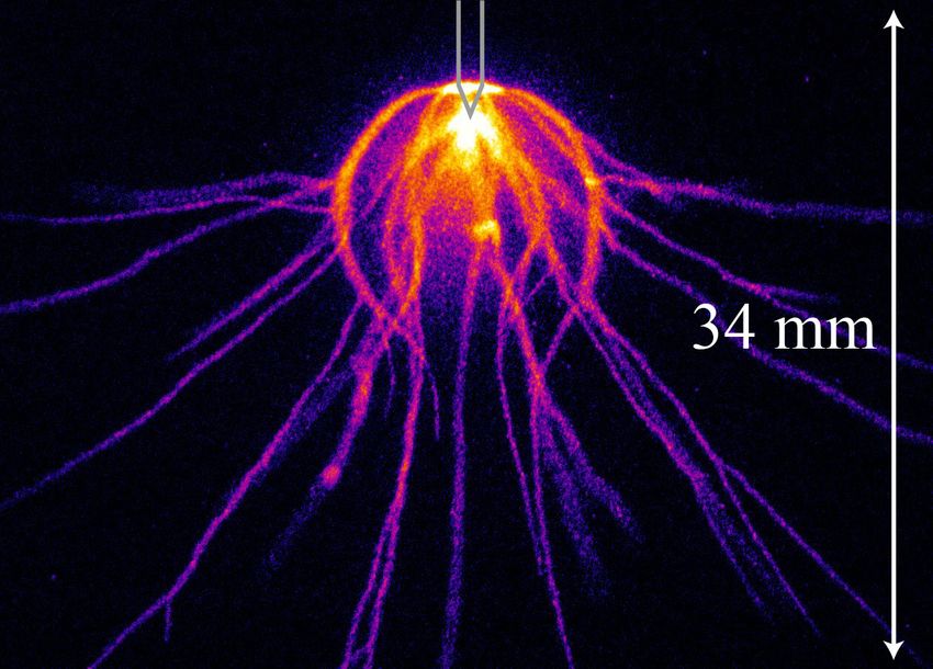
CONTENTS                                                                                                               2

Contents

1   Introduction                                                                                                        4
    1.1 Streamer phenomena in nature and technology . . . .        .   .   .   .   .   .   .   .   .   .   .   .   .    5
    1.2 A first view on the theory of streamers . . . . . . . .    .   .   .   .   .   .   .   .   .   .   .   .   .    6
         1.2.1 Impact ionization. . . . . . . . . . . . . . .      .   .   .   .   .   .   .   .   .   .   .   .   .    7
         1.2.2 Electron drift. . . . . . . . . . . . . . . . .     .   .   .   .   .   .   .   .   .   .   .   .   .    7
         1.2.3 Electric field enhancement. . . . . . . . . .       .   .   .   .   .   .   .   .   .   .   .   .   .    8
         1.2.4 Electron source ahead of the ionization front.      .   .   .   .   .   .   .   .   .   .   .   .   .    8
         1.2.5 Coherent structure. . . . . . . . . . . . . . .     .   .   .   .   .   .   .   .   .   .   .   .   .    9
    1.3 The multiple scales in space, time and energy . . . .      .   .   .   .   .   .   .   .   .   .   .   .   .    9
    1.4 Introduction to numerical models . . . . . . . . . . .     .   .   .   .   .   .   .   .   .   .   .   .   .   11
         1.4.1 Particle description of a discharge . . . . . .     .   .   .   .   .   .   .   .   .   .   .   .   .   11
         1.4.2 Fluid models . . . . . . . . . . . . . . . . .      .   .   .   .   .   .   .   .   .   .   .   .   .   12
    1.5 A first view on streamers in experiments . . . . . . .     .   .   .   .   .   .   .   .   .   .   .   .   .   12

2   The initial stage: Discharge inception                                                                             13
    2.1 Sources of free electrons . . . . . . . . . . . . . . . . . . . . . . . . . . . .                              14
    2.2 Avalanche-to-streamer transition far from boundaries . . . . . . . . . . . . .                                 16
         2.2.1 Starting with a single free electron. . . . . . . . . . . . . . . . . . .                               16
         2.2.2 Starting with many free or detachable electrons. . . . . . . . . . . .                                  17
    2.3 Streamer inception near surfaces . . . . . . . . . . . . . . . . . . . . . . . .                               18
    2.4 Inception cloud or diffuse discharge or spherical streamer or wide ionization
         front . . . . . . . . . . . . . . . . . . . . . . . . . . . . . . . . . . . . . . .                           19

3   Streamer propagation and branching                                                                                 20
    3.1 Positive versus negative streamers . . . . . . . . . . . .         .   .   .   .   .   .   .   .   .   .   .   20
    3.2 Streamer diameter and velocity . . . . . . . . . . . . . .         .   .   .   .   .   .   .   .   .   .   .   22
         3.2.1 Measurements.           . . . . . . . . . . . . . . . .     .   .   .   .   .   .   .   .   .   .   .   22
         3.2.2 Theory.         . . . . . . . . . . . . . . . . . . . .     .   .   .   .   .   .   .   .   .   .   .   24
    3.3 Electric currents . . . . . . . . . . . . . . . . . . . . . .      .   .   .   .   .   .   .   .   .   .   .   25
         3.3.1 Measurements. . . . . . . . . . . . . . . . . . .           .   .   .   .   .   .   .   .   .   .   .   25
         3.3.2 Theory. . . . . . . . . . . . . . . . . . . . . . .         .   .   .   .   .   .   .   .   .   .   .   25
    3.4 Electron density and conductivity in a streamer . . . . .          .   .   .   .   .   .   .   .   .   .   .   26
         3.4.1 Measurements. . . . . . . . . . . . . . . . . . .           .   .   .   .   .   .   .   .   .   .   .   26
         3.4.2 Theory. . . . . . . . . . . . . . . . . . . . . . .         .   .   .   .   .   .   .   .   .   .   .   26
    3.5 The stability field or the maximal streamer length . . . .         .   .   .   .   .   .   .   .   .   .   .   27
    3.6 Stepped propagation of negative streamers . . . . . . . .          .   .   .   .   .   .   .   .   .   .   .   27
    3.7 Streamer paths . . . . . . . . . . . . . . . . . . . . . .         .   .   .   .   .   .   .   .   .   .   .   29
    3.8 Streamer interaction . . . . . . . . . . . . . . . . . . . .       .   .   .   .   .   .   .   .   .   .   .   31
    3.9 Streamer branching . . . . . . . . . . . . . . . . . . . .         .   .   .   .   .   .   .   .   .   .   .   32
         3.9.1 Experimental results for positive streamer in air.              .   .   .   .   .   .   .   .   .   .   32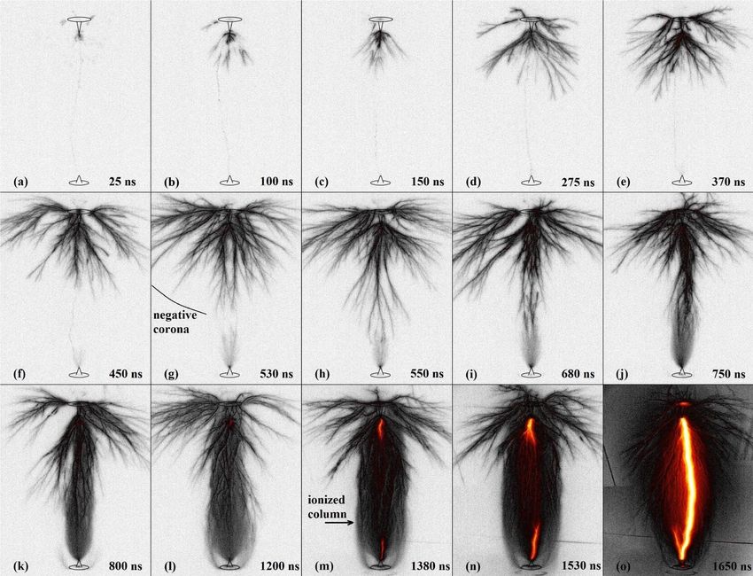
CONTENTS                                                                                                        3

         3.9.2 Theoretical understanding of streamer branching.           . . . . . . . . .                     34
         3.9.3 Streamer branching in other gases and background-ionizations.            . .                     35
         3.9.4 Branching due to macroscopic perturbations and peculiar events.            .                     35
    3.10 Interaction with dielectric surfaces . . . . . . . . . . . . . . . . . . . . . . .                     36

4   Streamers in different media and pressures                                                                  37
    4.1 Streamers in different gases . . . . . . . . . . . . . . . . . . . . . . . . . . .                      37
    4.2 Scaling with gas number density and its range of validity . . . . . . . . . . .                         37
    4.3 Discharges in liquid and solids. . . . . . . . . . . . . . . . . . . . . . . . . .                      39

5   Other topics                                                                                                39
    5.1 Plasma theory and electrostatic approximation . . . . . . . . .         .   .   .   .   .   .   .   .   39
    5.2 Basic streamer plasma chemistry . . . . . . . . . . . . . . . .         .   .   .   .   .   .   .   .   41
    5.3 Interaction with gas flow and heat . . . . . . . . . . . . . . .        .   .   .   .   .   .   .   .   42
        5.3.1 Streamers in hot gases.       . . . . . . . . . . . . . . .       .   .   .   .   .   .   .   .   42
        5.3.2 Gas heating by streamers and the transition to leaders.               .   .   .   .   .   .   .   43
        5.3.3 Gas flow induced by streamers and the corona wind.                    .   .   .   .   .   .   .   43
    5.4 High-energy phenomena . . . . . . . . . . . . . . . . . . . .           .   .   .   .   .   .   .   .   45
        5.4.1 Electron runaway. . . . . . . . . . . . . . . . . . . .           .   .   .   .   .   .   .   .   45
        5.4.2 X- and γ-rays, anisotropy and discharge polarity. . . .           .   .   .   .   .   .   .   .   45
        5.4.3 High energy phenomena in pulsed discharges. . . . . .             .   .   .   .   .   .   .   .   46
    5.5 Plasma jets . . . . . . . . . . . . . . . . . . . . . . . . . . .       .   .   .   .   .   .   .   .   46
    5.6 Sprite discharges in the upper atmosphere . . . . . . . . . . .         .   .   .   .   .   .   .   .   47

6   Recent advances in streamer simulations                                                                     47
    6.1 Particle (PIC-MCC) models . . . . . . . . . . . . . . . . .         .   .   .   .   .   .   .   .   .   49
    6.2 Fluid models . . . . . . . . . . . . . . . . . . . . . . . . .      .   .   .   .   .   .   .   .   .   51
         6.2.1 Transport and reaction coefficients . . . . . . . . . .      .   .   .   .   .   .   .   .   .   51
         6.2.2 Source terms . . . . . . . . . . . . . . . . . . . . .       .   .   .   .   .   .   .   .   .   52
         6.2.3 Comparison of fluid models for streamer discharges           .   .   .   .   .   .   .   .   .   52
         6.2.4 Time stepping . . . . . . . . . . . . . . . . . . . . .      .   .   .   .   .   .   .   .   .   53
         6.2.5 Spatial discretization . . . . . . . . . . . . . . . . .     .   .   .   .   .   .   .   .   .   53
    6.3 Hybrid models . . . . . . . . . . . . . . . . . . . . . . . .       .   .   .   .   .   .   .   .   .   54
    6.4 Macroscopic models . . . . . . . . . . . . . . . . . . . . .        .   .   .   .   .   .   .   .   .   54
    6.5 Numerical grid and adaptive refinement . . . . . . . . . . .        .   .   .   .   .   .   .   .   .   56
    6.6 Field solvers . . . . . . . . . . . . . . . . . . . . . . . . . .   .   .   .   .   .   .   .   .   .   58
         6.6.1 Field solvers for uniform grids . . . . . . . . . . . .      .   .   .   .   .   .   .   .   .   58
         6.6.2 Field solvers for structured grids with refinement . .       .   .   .   .   .   .   .   .   .   59
         6.6.3 Field solvers on unstructured grids . . . . . . . . . .      .   .   .   .   .   .   .   .   .   59
    6.7 Computational approaches for photo-ionization . . . . . . .         .   .   .   .   .   .   .   .   .   59
    6.8 Modeling streamer chemistry and heating . . . . . . . . . .         .   .   .   .   .   .   .   .   .   60
    6.9 Simulating streamers interacting with surfaces . . . . . . . .      .   .   .   .   .   .   .   .   .   61
    6.10 Validation and verification in discharge simulations . . . . .     .   .   .   .   .   .   .   .   .   61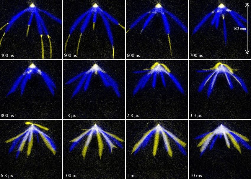
CONTENTS                                                                                                                             4

               Figure 1. A long exposure, false colour, image of a peculiar streamer discharge caused by a
               complex voltage pulse. Image taken from [1].

7   Modern streamer diagnostics                                                                                                      62
    7.1 Electrical diagnostics . . . . . . . . . . . .       .   .   .   .   .   .   .   .   .   .   .   .   .   .   .   .   .   .   63
    7.2 Optical imaging techniques . . . . . . . . .         .   .   .   .   .   .   .   .   .   .   .   .   .   .   .   .   .   .   63
        7.2.1 Measuring diameters and velocities             .   .   .   .   .   .   .   .   .   .   .   .   .   .   .   .   .   .   65
    7.3 Optical Emission Spectroscopy . . . . . . .          .   .   .   .   .   .   .   .   .   .   .   .   .   .   .   .   .   .   66
    7.4 Laser diagnostics . . . . . . . . . . . . . .        .   .   .   .   .   .   .   .   .   .   .   .   .   .   .   .   .   .   67
    7.5 Other diagnostics . . . . . . . . . . . . . .        .   .   .   .   .   .   .   .   .   .   .   .   .   .   .   .   .   .   68

8   Outlook and open questions                                                                                                       70
    8.1 Discharge inception: . . . . . . . . . . . . . . .               .   .   .   .   .   .   .   .   .   .   .   .   .   .   .   70
    8.2 Streamer evolution . . . . . . . . . . . . . . . .               .   .   .   .   .   .   .   .   .   .   .   .   .   .   .   70
    8.3 Further evolution after passage of ionization front              .   .   .   .   .   .   .   .   .   .   .   .   .   .   .   71
    8.4 Particular physical mechanisms . . . . . . . . . .               .   .   .   .   .   .   .   .   .   .   .   .   .   .   .   71

1. Introduction

Streamers are fast-moving ionization fronts that can form complex tree-like structures or other
shapes, depending on conditions (see e.g. figure 1). In this paper, we review our present
understanding of streamer discharges. We start from the basic physical mechanisms and
concepts, aiming also at beginners in the field. We also touch on related phenomena such as
discharge inception, diffuse discharges, nanosecond pulsed discharges, plasma jets, transient
luminous events and lightning propagation, electron runaway and high energy radiation.
     The paper is organized as follows: In the present introductory section we briefly review
streamer phenomena in nature and technology, we discuss the relevant physical mechanisms
with their multiscale nature and we have a first look at numerical models and streamers in
laboratory experiments. The following two sections are devoted to the details of the different
temporal stages of the discharge evolution: discharge inception (section 2) and streamer
propagation and branching (section 3). In these two sections we mainly concentrate on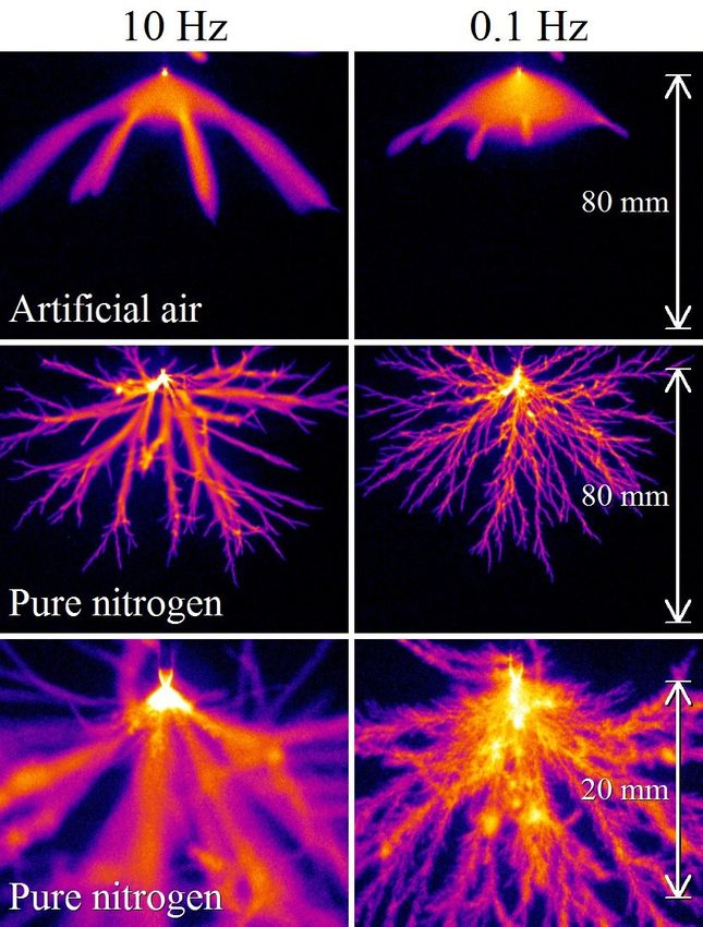
CONTENTS                                                                                       5

streamers in (ambient) air but in section 4 we treat streamers in other media and pressures. In
section 5 this is followed by discussions on streamer-relevant plasma theory and chemistry,
interaction with flow and heat, high energy phenomena, plasma jets and sprite discharges.
The final main sections treat the available methods in detail, first in modeling and simulations
(section 6), and then in plasma diagnostics (section 7). We end with a short outlook and an
overview of open questions on the physics of streamer discharge phenomena (section 8).

1.1. Streamer phenomena in nature and technology

The most common and well-known occurrence of streamers is as the precursor of sparks
where they create the first ionized path for the later heat-dominated spark discharge. Streamers
play a similar role in the inception and in the propagation of lightning leaders.Streamers
are directly visible in our atmosphere as so-called sprites, discharges far above active
thunderstorms; they will be discussed in more detail in section 5.6.
      Streamers are members of the cold atmospheric plasma (CAP) discharge family. Most
industrial applications of streamers and other CAPs (i.e., not as precursors of discharges like
sparks) utilize the unique chemical properties of such discharges. The highly non-equilibrium
character and the resulting high electron energies enable CAPs to start high-temperature
chemical reactions close to room temperature. This leads to two major advantages compared
to thermal plasmas and other hot reactors: firstly it enables such reactions in environments that
cannot withstand high temperatures, and secondly it can make the chemistry very efficient as
no energy is lost on gas heating.
      The electrons that trigger the chemical reactions can have energies of the order of 10 eV
or higher, something that cannot be achieved in any thermal process (as 1 eV corresponds
to 11600 Kelvin). In air and air-like gas mixtures this leads to the production of OH, O
and N radicals as well as of excited species and ions like O−2 , O− , O+ , N+4 and O+4 after an
initial production of N+2 , O+2 , see section 5.2. Each of these species can start other chemical
reactions, either within the bulk gas, on nearby surfaces or even in nearby liquids when the
species survives long enough and can be easily absorbed. The initial energy distribution of
the generated excited species is typically far from thermal equilibrium.
      Due to these properties of streamers and other CAPs they are used or developed for
a myriad of applications, most of which are described extensively in the following review
papers [2, 3, 4, 5]. Popular applications are plasma medicine [6, 7, 8] including cancer
therapy [9] and sterilization [10], industrial surface treatment [11], air treatment for cleaning
or ozone production [12, 13], plasma assisted combustion [14, 15] and propulsion [16, 17]
and liquid treatment [18, 19]. Two recent reviews on nanosecond pulsed streamer generation,
physics and applications are by Huiskamp [20] and Wang and Namihira [21].
      A fast pulsed discharge like a streamer has the advantage that the electric field is not
limited by the breakdown field. The electric field and thereby the electron energy can
transiently reach much higher values than in static discharges. Pulsed discharges can be
seen as energy conversion processes, as sketched in Figure 2. First, pulsed electric power
is applied to gas at (close to) atmospheric pressure. When the gas discharge starts to develop,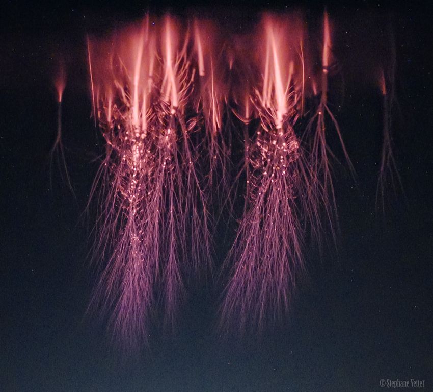
CONTENTS                                                                                               6

                     Pulsed electric power

                          Energetic                    Collisions with
                          electrons                    gas molecules

          Electron                                           Plasma                    Electric
                                  Corona wind
          runaway                                           chemistry                 breakdown

                                Plasma actuators             Plasma:                 High-voltage
                                                            medicine,                switch gear,
                                                           agriculture,               lightning
                                                           combustion,                protection
                                                           disinfection,
                                                           air cleaning

               Figure 2. Energy conversion in pulsed atmospheric discharges with application fields.

this energy is converted to ionization and to free electron energies in the eV range, far from
thermal equilibrium. The further plasma evolution can include different physical and chemical
mechanisms. a) If the local electric field is high enough, electrons can keep accelerating up
to electron runaway, and create Bremsstrahlung photons in collisions with gas molecules;
the photons can initiate other high-energy processes in the gas, as is in particular seen in
thunderstorms, see section 5.4. b) The drift of unbalanced charged particles through the gas
can create so-called corona wind, see section 5.3. c) Excitation, ionization and dissociation
of molecules by electron impact trigger plasmachemical reactions in the gas, see section 5.2.
d) Electric breakdown means that the conductivity increases further by ionization, heating
and thermal gas expansion; it is used in high voltage switch gear, and has to be controlled in
lightning protection.
     Streamer discharges are often produced in ambient air. For this reason, we and many
other authors use the term Standard Temperature and Pressure (STP) as a simple definition of
ambient (air) conditions. Its exact definition varies, but it always represents a temperature of
either room temperature or 0◦ C and a pressure close to 1 atmosphere.

1.2. A first view on the theory of streamers

In this section we will discuss the basics of streamer discharges. The theory presented here
is primarily based on streamers in atmospheric air, but most of the concepts are also valid for
(or can be generalized to) other gas densities and/or compositions.
      Streamer discharges can appear when a gas with low to vanishing electric conductivity
is suddenly exposed to a high electric field. Key for streamer discharges are the acceleration
of electrons in the local electric field and the collisions between electrons and neutral gas
molecules (for brevity, we will use the term gas molecules instead of writing gas atoms or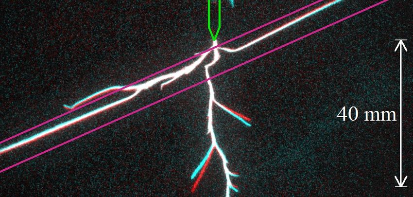
CONTENTS                                                                                         7

molecules), which can be of the following type:
  • Elastic collisions, in which the total kinetic energy is conserved, although some of it is
    typically transferred from the electron to the gas molecule.
  • Excitations, in which some of the electron’s kinetic energy is used to excite the molecule.
    Depending on the gas molecule (or atom), there can be rotational, vibrational and
    electronic excitations.
  • Ionization, in which the gas molecule is ionized.
  • Attachment, in which the electron attaches to the gas molecule, forming a negative ion.
Data for the collisions of electrons with different types of atoms and molecules can be found,
e.g., on the community webpage www.lxcat.net.
      As explained below, streamer discharges can form where the electric field is above the
breakdown value. However, streamers can also enter into regions where the electric field is
below breakdown. This is due to the nonlinear streamer mechanism, which is based on the
following physical processes.

1.2.1. Impact ionization. Free electrons that are accelerated by a high local electric field,
can create new electron-ion pairs when they impact with sufficient kinetic energy on gas
molecules. If there is also an electron attachment reaction, then the impact ionization rate
must be larger than the attachment rate for the plasma to grow; the local electric field is then
said to be above the breakdown value. In such fields, the chain reaction of ionization growth
leads to the creation of electrically conducting plasma regions.
     How many ionization and attachment events occur per electron per unit length is
described by the ionization and attachment coefficients α and η. As discussed above,
breakdown requires that α > η, or in other words, that the effective ionization coefficient
               ᾱ = α − η                                                                      (1)
is positive. The electric field Ek where the effective ionization coefficient vanishes ᾱ(Ek ) = 0,
is called the classical breakdown field; for E > Ek , the ionization density grows.
      In electronegative gases like air, electron loss due to recombination is negligible relative
to attachment, because recombination is quadratic in the degree of ionization, and the degree
of ionization is small.

1.2.2. Electron drift. Electrons gain kinetic energy in the local field and lose energy in
collisions with gas molecules. This leads to an average drift motion that can be described
by vdrift = −µe E, where µe is the electron mobility. Only in very high fields, electrons can
overcome the friction barrier caused by collisions; they then keep accelerating and become
runaway electrons (for further discussion see section 5.4).
      The drift motion of charged particles in the field leads to an electric current that usually
satisfies Ohm’s law
               j = σE,                                                                         (2)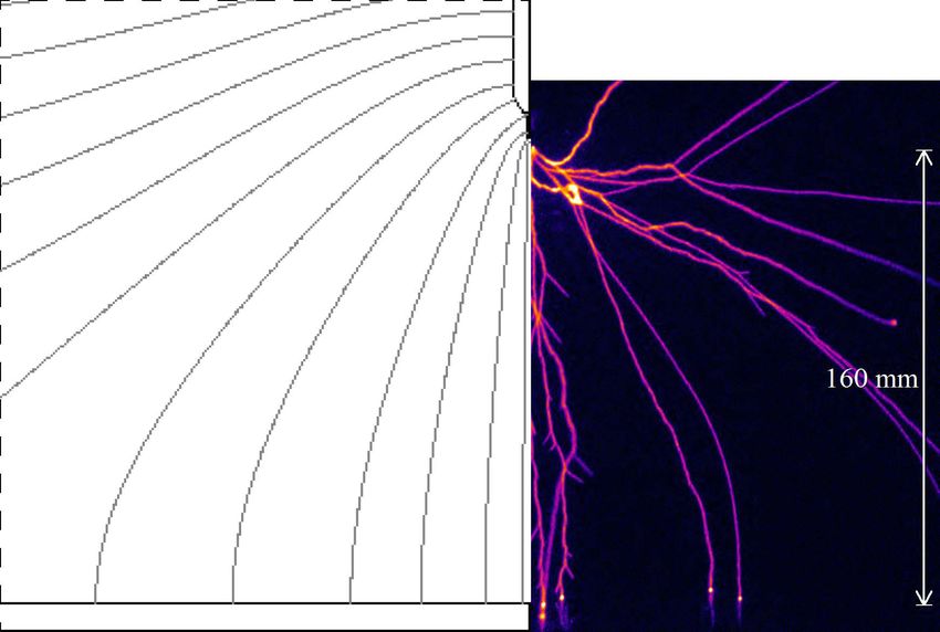
CONTENTS                                                                                        8

where j is the electric current density and σ the conductivity of the plasma. Note that magnetic
fields are not taken into account here, as their effect is typically negligible, see section 5.1.
     As long as electron and ion densities are similar (i.e., during and after the ionization
process and before attachment depletes the electrons), the electron contribution dominates the
conductivity, hence σ ≈ eµe ne , where e is the elementary charge and ne the electron density.
Ions also drift in the field, but as they carry the same electric charge and are much heavier,
they are much slower than the electrons. Furthermore, ions lose kinetic energy more easily
than electrons as they have a similar mass as the gas molecules they collide with. (This is a
consequence of the conservation of energy and momentum in collisions.)

1.2.3. Electric field enhancement. Equation (2) shows that in an ionized medium or plasma
with conductivity σ, an electric field creates an electric current. Due to the conservation of
electric charge
               ∂t ρ + ∇ · j = 0,                                                              (3)
the charge density distribution ρ changes in time due to a current density j, and the electric
field E changes as well according to Gauss’ law of electrostatics (in vacuum or in not too
dense gases, in the absence of solid or liquid bodies)
               ∇ · E = ρ/0 ,                                                                 (4)
where 0 is the dielectric constant.
    Equations (2)–(4) imply that the interior of a non-moving body with constant
conductivity σ is screened on the time scale of the dielectric relaxation time
               τ = 0 /σ,                                                                     (5)
while a surface charge builds up at the edges that screens the field in the interior. If the shape
of the conducting body is elongated in the direction of the electric field, there is significant
surface charge around the sharp tips, and therefore a strong field enhancement ahead of these
tips. If the locally enhanced field at a tip exceeds the breakdown value Ek , a conducting
streamer body can grow at such a location, even if the background field is below breakdown.
This is illustrated with numerical modeling results in figure 3.
     To be more precise, there are two important corrections to this simple picture of a
streamer: first, the ionization and hence the conductivity of a streamer is not constant, but
changes in space and time, and for a generalization of the dielectric relaxation time to a
reactive plasma with ᾱ > 0, we refer to [23]. Second, the shape of the conducting body
changes in time, and therefore the electric field is typically not completely screened from the
interior.

1.2.4. Electron source ahead of the ionization front. The above mechanisms suffice to
explain the propagation of negative (i.e., anode-directed) streamers in the direction of electron
drift. However, positive (i.e., cathode-directed) streamers frequently move with similar
velocity against the electron drift direction. They require an electron source ahead of the
ionization front. The dominant mechanism in air is photo-ionization, a nonlocal mechanism.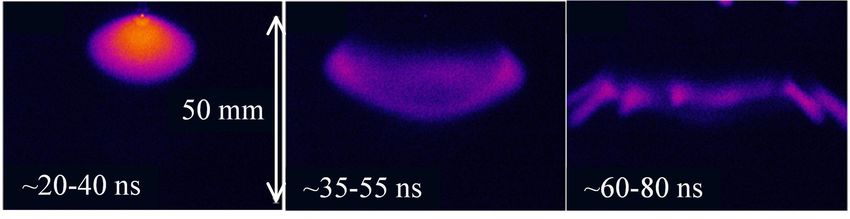
CONTENTS                                                                                                    9

               Figure 3. Simulation example showing a cross section of a positive streamer propagating
               downwards. A strong electric field is present at the streamer tip. A charge layer surrounds
               the streamer channel, with both positive charge (blue) and negative charge (red) present. A
               cross section of the instantaneous light emission is also shown, which is concentrated near the
               streamer head. The simulation was performed with an axisymmetric fluid model [22] in air at
               1 bar, in a gap of 1.6 cm with an applied voltage of 32 kV.

Photons are generated in the active impact ionization region at the streamer tip, but create
electron-ion pairs at some characteristic distance determined by their absorption cross-section.
Other sources of free electrons ahead of a streamer ionization front can be earlier discharges,
external radiation sources like radioactivity or cosmic rays, electron detachment from negative
ions, or bremsstrahlung photons from runaway electrons.

1.2.5. Coherent structure. The nonlinear interaction of impact ionization, electron drift and
field enhancement creates the streamer head, see Figure 3. It can be considered as a coherent
structure that propagates with a dynamically stabilized shape. Other examples of coherent
structures are solitons or chemical or combustion fronts.

1.3. The multiple scales in space, time and energy

The multiple spatial scales in a streamer discharge are illustrated in Figure 4. From small to
large, the following processes take place:
     Collisions: On the most microscopic level (panel a), electrons that are accelerated by the
electric field collide with gas molecules. A proper characterization of the collision processes
is key to understanding the electron energy distribution as well as the excitation, ionization
and dissociation of molecules.
     Motion of an ensemble of electrons: Panel b in Figure 4 shows an ensemble of
“individual” electrons moving in an electric field, colliding with gas molecules, and forming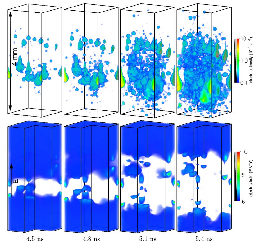
CONTENTS                                                                                                 10

                                                a)
                          b)

                                                     e-

                                           c)

                                                              d)

               Figure 4. The multiple spatial scales in streamer discharges: a) collision of an electron with
               an atom or molecule, b) multiple electrons accelerate in a local electric field, collide with
               neutral gas molecules and form an ionization avalanche, c) a branching streamer discharge
               with field enhancement at the tips, d) a discharge tree with multiple streamer branches. Panel
               d is reproduced from a figure in [24].

an ionization avalanche. The modeling of such electrons with Monte Carlo particle methods
is described in sections 1.4.1 and 6.1.
     Field enhancement and streamer mechanism: Panel c in Figure 4 illustrates a streamer
discharge with local field enhancement at the channel tips, as described above. The picture
shows the result of a 3D simulation [22]. Such simulations are often performed with fluid
models, which use a density approximation for electrons and ions, see sections 1.4.2 and 6.2.
     Multi-streamer structures: In most natural and technical processes, streamers do not
come alone, and they interact through their space charges and their internal electric currents.
A reduced model that approximates the growing streamer channels as growing conductors
with capacitance is shown in panel d of Figure 4 and discussed in more detail in section 6.4;
such so-called fractal models are a key to understanding processes with hundreds or more
streamers.
     Different scales in time and energy: A pulsed discharge starts from single electrons
and avalanches, and eventually develops space charge effects to form a streamer. Later,
behind the streamer ionization front, the ion motion, the deposited heat and consecutive
gas expansion, and the initiated plasma-chemistry become important. These mechanisms
can cause a transition to a discharge with a higher gas temperature and a higher degree of
ionization. Such discharges are known as leaders, sparks and arcs.
     The electron energy scales depend on the local electric field and are much higher at the
streamer tip than elsewhere, but typically in the eV range. However, electron runaway can
accelerate electrons into the range of tens of MeV in the streamer-leader phase of lightning,
in a not yet fully understood process.
CONTENTS 11
In sections 2, 3 and 5.3, we will discuss the temporal sequence of physical processes in
a pulsed discharge in detail.
1.4. Introduction to numerical models
We now briefly introduce two types of models that are often used to simulate streamer
discharges: fluid and particle models. A more detailed description of these models and their
range of validity can be found in section 6.
1.4.1. Particle description of a discharge Microscopically, the physics of a streamer
discharge is determined by the dynamics of particles: electrons, ions, neutral gas molecules
(or atoms) and photons. The electrons and ions interact electrostatically through the
collectively generated electric field. Their momentum p and energy ε change in time as
∂t p = qE,
∂t ε = qv · E,
where q is the particle’s charge and v its velocity. The energy and momentum gained from the
field is however quickly lost in collisions with neutral gas molecules. As the typical degree of
ionization in streamers at up to 1 bar is below 10−4 (see sections 3.4 and 4.2), charged particles
predominantly collide with neutrals rather than with other charged particles. In a particle-in-
cell (PIC) code for streamer discharges, it is therefore common to describe the electrons as
particles that move and collide with neutrals, the slower ions as densities, and the neutrals
as a background density. To reduce computational costs, each simulation particle typically
represents multiple physical electrons. The neutral gas is included only implicitly through the
collision rates for electron-neutral scattering, excitation, ionization and attachment collisions.
In a PIC code, the electron and ion densities are used to compute the charge density ρ
on a numerical mesh. The electric potential φ and the electric field E = −∇φ can then be
computed by solving Poisson’s equation
∇ · (ε∇φ) = −ρ, (6)
with suitable boundary conditions, where ε is the dielectric permittivity. Note that the
electrostatic approximation is used here; its validity is discussed in section 5.1.
Compared to fluid models, the main drawback of particle models is their higher
computational cost. Particle models have several important advantages, however:
• They can be used when there are few particles, so that a density approximation is
not valid. This is for example relevant during the inception phase of a discharge, see
section 2.
• Stochastic processes can be described properly. Such processes include not only the
electron-neutral collisions, but for example also the photo-ionization mechanism. If there
are few photoionization events, their stochasticity can contribute to streamer branching,
see section 3.9.CONTENTS 12
• The distribution of electrons in physical and velocity space is directly approximated,
whereas additional assumptions are required in a fluid model, which may not be valid.
For more details about particle models, see section 6.1.
1.4.2. Fluid models Fluid models employ a continuum description of a discharge, which
means that they describe the evolution of one or more densities in time. In the classic drift-
diffusion-reaction model, the electron density ne evolves as
∂t ne = ∇ · (ne µe E + De ∇ne ) + S e + S ph , (7)
where De is the electron diffusion coefficient and S ph is a source term accounting for nonlocal
photo-ionization. The source term S e corresponds to electron impact ionization α and
attachment η, and is usually given by
S e = ᾱµe Ene , ᾱ = α − η, (8)
where E = |E|. Depending on the gas composition, one or more ion species can be generated.
In the simplest case, no additional reactions for these ions are included, and they are assumed
to be immobile. A single density ni that describes the sum of positive minus negative ion
densities can then be used, which changes in time as
∂t ni = S e + S ph . (9)
Due to the conservation of electric charge, the source terms have to be equal in equations (7)
and (9).
The transport coefficients (µe and De ) and the source term S e in equation (7) depend on
the electron velocity distribution. They are often parameterized using the local electric field
or the local mean energy, see section 6.2. Details about the computation of photo-ionization
are given in section 6.7. An example of a simulation of a positive streamer discharge in
atmospheric air with the classic fluid model is shown in figure 3.
It should be noted that the reactions in the classical discharge model only contain
interactions of discharge products (like electrons, ions or photons) with neutrals, and not
directly with each other, except through the electric field. The reason is that the degree of
ionization in a streamer at up to atmospheric pressure is typically below 10−4 . Processes that
are quadratic or higher in the degree of ionization are therefore negligible. This is discussed
in more detail in section 4.2.
1.5. A first view on streamers in experiments
We have started with models, because they allow understanding how microscopic mechanisms
interact to create the inner nonlinear structure of a single streamer. The challenge for modeling
lies in covering multi-streamer processes and discharge phenomena on earlier and later time
scales (that will be addressed in later sections) based on proper micro-physics input.
For experiments, the situation is quite the opposite: It is easier to observe phenomena
with many streamers over longer times than to zoom into the inner structure of single streamerCONTENTS 13
Figure 5. Example of ICCD images for positive streamer discharges under the same conditions
using different gate (exposure) times, as indicated on the images. The camera delay has been
varied so that the streamers are roughly in the centre of the image. The discharges were
captured in artificial air at 200 mbar with a voltage pulse of about 24.5 kV. Image from [25].
tips on the intrinsic (nanosecond) time scale. Therefore, all streamer experimental images
shown here are of complete discharges containing one or more streamer channels.
The easiest to acquire, and therefore the most often shown quantity in streamer
experiments is the light emission. Light can easily be imaged by ICCD or other cameras (see
sections 7.2 and 4.1 for limitations). In air, a camera will only image the actively growing
regions of a streamer discharge, i.e., the tips, while the current carrying channels mostly stay
dark, as the electric fields and hence the electron energies are too low in the channels to excite
the molecules to emissions in the optical range. This effect is demonstrated in figure 5 where
for short exposures only small dots are visible.
Figure 6 shows long exposure images of streamers in different gases and pressures. It
showcases the wide variety of shapes and sizes of streamers, ranging from single channels to
complex streamer trees at higher pressures. It also shows the variability in streamer width and
branching behaviour between the different conditions.
Two examples of the development of a streamer discharge at an applied voltage of 1 MV
over a distance of 1 m in ambient air can be seen in figure 7. The top panel shows positive
streamers propagating smoothly from the top (HV) electrode to the ground bottom electrode,
which are, in the end, met by short negative counter-propagating streamers and then grow into
a hot, spark-like channel. The bottom panel shows that negative streamer expansion from the
top electrode instead happens in bursts, likely related to the microsecond voltage rise time (see
section 3.5). Almost simultaneously, positive streamers are growing from the elevated bottom
electrode. These meet each other after around 550 ns, again forming a spark-like channel.
2. The initial stage: Discharge inception
The formation of a discharge requires two conditions: First, a sufficiently high electric field
should be present in a sufficiently large region. Second, free electrons should be present in this
region. If no or few of these electrons are present, the discharge may form with a significant
delay or not at all. On the other hand, a sufficient supply of free electrons can reduce the
inception delay and jitter, and also the required electric field to start a discharge within a
given time.CONTENTS 14
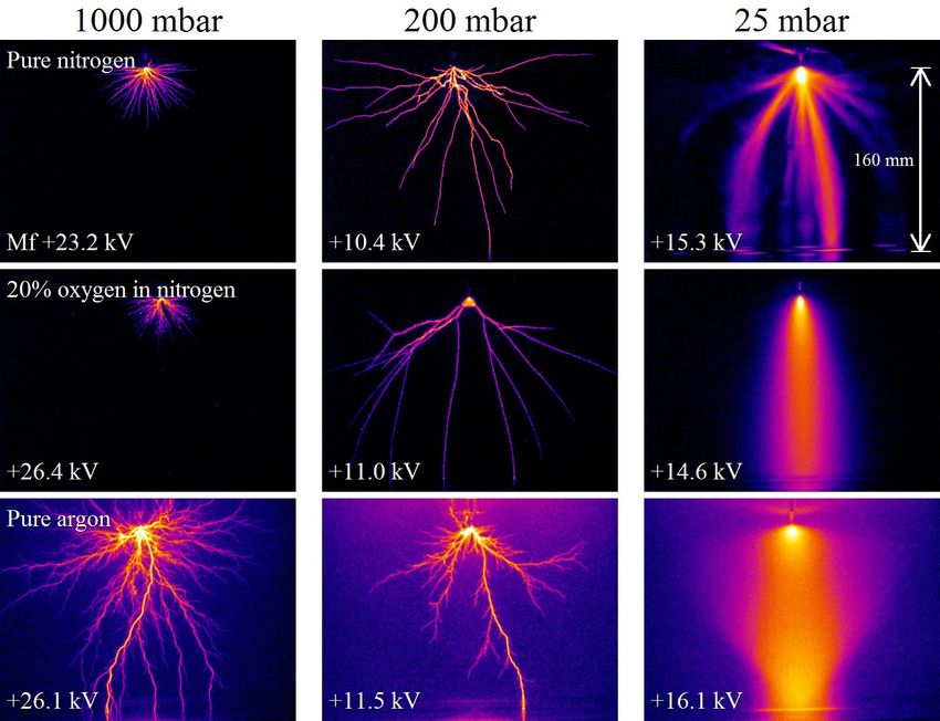
Figure 6. Overview of positive streamer discharges produced in three different gas mixtures
(rows), at 1000, 200 and 25 mbar (columns). All measurements have a long exposure time and
therefore show the whole discharge, including transition to glow for 25 mbar. Image adapted
from [26].
Below, we will first discuss possible sources of free electrons, and then the conditions on
the electric field to start a discharge, both in the bulk and near a surface. Finally, we discuss
inception clouds, a stage immediately before streamer emergence near a pointed electrode in
air.
2.1. Sources of free electrons
In repetitive discharges, one discharge can serve as an electron source for the next discharge.
Depending on the time span between them, some electrons can still be present, or they can
detach from negative ions like O−2 or O− in air, or they can be liberated through Penning
ionization. Another possibility is storage on solid surfaces.
For the first discharge in a non-ionized gas, possible electron sources are the decay of
radioactive elements within the gas or external radiation. The actual mechanisms depend
on local circumstances. E.g., in the lab, the materials used for the vessel and the lab itself,
together with possible radioactive gas admixtures, determine the local radiation level. UVCONTENTS 15
Figure 7. Development of positive (top panel) and negative (bottom panel) streamers creating
a high-voltage spark in gap lengths of 100 and 127 cm respectively at applied voltages of 1.0
and 1.1 MV respectively, both with a voltage rise time of 1.2 µs in atmospheric air. Each
picture shows a different discharge under the same conditions with increasing exposure time
from discharge inception. In the top panel these times are (for a-j): 70, 160, 190, 250, 320,
340, 370, 410, 460 and 610 ns. In the bottom panel they are indicated on the images. Images
from [27] and [28].CONTENTS 16
light can supply electrons as well, especially from surfaces which can emit for much lower
photon energies than gases.
In the Earth’s atmosphere, the availability of free electrons strongly depends on altitude;
we discuss it here in descending order. Above about 85 km at night time or about 40 km
at day time, the D and the E layer of the ionosphere contain free electrons. In fact, the
lower edge of the E layer at night time can sharpen under the action of electric fields from
active thunderstorms, and launch sprite discharges downward which are upscaled versions
of streamers at very low air densities [29, 30, 31], see also section 5.6. On the other hand,
electrons are scarce at lower altitudes, as they easily attach to oxygen molecules. In particular,
in wet air, water clusters grow around these ions and electron detachment is very unlikely [32].
On the other hand, when a high energy cosmic particle enters our atmosphere, it can liberate
large electron numbers in extensive air showers which could be a mechanism for lightning
inception [33]. Up to 3 km altitude, the radioactive decay of radon from the ground is the
main source of free electrons [34], except for specific local soil conditions.
2.2. Avalanche-to-streamer transition far from boundaries
2.2.1. Starting with a single free electron. The simplest case to consider is a single free
electron in a gas in a homogeneous field. According to equations (7) and (8), the ionization
avalanche grows if the effective Townsend ionization coefficient ᾱ in a given electric field
strength E is positive, i.e., if E > Ek . During a time t, the centre of an avalanche drifts a
distance d = µe Et in the electric field, and the number of electrons is multiplied by a factor
exp (ᾱ(E) d).
Eventually, the space charge density of the avalanche creates an electric field comparable
to the external field. At this moment, space charge effects have to be included, and the
discharge transitions into the streamer phase. In ambient air, this happens when ᾱ(E)d ≈ 18;
this is known as the Meek criterion. The avalanche to streamer transition is analyzed in [35].
In particular, it was found that electron diffusion yields a small correction to the Meek number,
and that it determines the width of avalanches. (In contrast, Raizer [36] relates the width of
avalanches to electrostatic repulsion which is not consistent with the concept that their space
charge is negligible.)
When a single electron develops an avalanche in an inhomogeneous electric R field E(r),
the local multiplication rates ᾱ(E) add up over the electron trajectory L like L ᾱ(E(s)) ds.
The Meek criterion for the avalanche to streamer transition in air at standard temperature and
pressure is then
Z
ᾱ(E(s)) ds ≈ 18. (10)
L
The Meek number gets a logarithmic correction in the gas number density when it deviates
from atmospheric conditions [35]. This follows from the scaling laws discussed in section
4.2.
If there are Ne electrons starting together from about the same location, the required
electron multiplication for an avalanche to streamer transition decreases with log Ne , since theCONTENTS 17
Figure 8. Simulation of discharge inception in atmospheric air in a field of twice the
breakdown value, taken from [37]. Shown are the electron density (top) and electric field
(bottom). Initially, a layer of O−2 ions with a density of 104 cm−3 was present. Electrons detach
from these ions and form multiple overlapping avalanches.
hR i
criterion becomes Ne exp L
ᾱ(E(s)) ds ≈ exp(18).
2.2.2. Starting with many free or detachable electrons. When the initial condition is a
wide spatial distribution of electrons in an electric field above breakdown, streamer formation
competes with a more homogeneous breakdown due to many overlapping ionization
avalanches. Such a situation can arise when there is still a substantial electron density from
a previous discharge, or when electrons detach from ions in the applied electric field. The
dynamics of a pre-ionized layer developing into an ionized and screened region through a
multi-avalanche process are shown in figure 8. While the Meek number characterizes the
critical propagation length of an avalanche for space charge effects to set in, the ionization
screening time [23]
ᾱ0 E
!
τis = ln 1 + /(ᾱµe E) (11)
en0
is the temporal equivalent for a multi-avalanche process, where n0 is the initial electron
density and E the applied electric field. The ionization screening time can be seen as the
generalization of the dielectric relaxation time (5) to an electron density that changes in timeCONTENTS 18
due to the effective impact ionization ᾱ.
In the past, many authors have simulated streamers in electric fields above the breakdown
value. This was often done to reduce computational costs, since such streamers can be
simulated within shorter times in smaller computational domains. However, the results of
such simulations can change substantially if background ionization is added, since streamer
breakdown and the homogeneous breakdown mode of Figure 8 are competing when the
background field is above breakdown.
On the other hand, if the electric field is below breakdown, discharges would mostly not
start. However, if there is a sufficiently high and compact density of electrons and ions, this
ionized patch can screen the electric field from its interior and enhance it at its edges. This
leads to a local electron multiplication and drift only in the region above breakdown, and to
the emergence and growth of a positive streamer at one side of the initial plasma, while the
negative streamer on the opposite side is delayed if it grows at all.
The basic differences between discharge inception below and above the breakdown field
are discussed in more detail in [37].
2.3. Streamer inception near surfaces
Above, we have discussed discharge inception within the gas, far from any boundaries.
However, many discharges ignite near dielectric or conducting surfaces, such as electrode
needles or wires, water droplets or ice particles, because the electric field near such objects
is enhanced. For the same shape and material, positive discharges ignite more easily than
negative ones, at least in air.
The inception process again is determined by the availability of free electrons near
the surface and by their avalanche growth. As discussed above, the electron number in an
avalanche grows as the exponent of L ᾱ(E)ds where the integral is taken over the avalanche
R
path L along an electric field line. The Meek number is calculated on the path L that has the
largest value of the integral and ends at the surface. In electrical engineering, it is known from
experiments that a discharge near a strongly curved electrode can start when the Meek number
is as low as 9 or 10 [38, 39, 40, 41, 42], but apparently this is not known to geophysicists
modeling lightning inception near ice particles in thunderclouds [43, 44] who use a Meek-
number of 18 for their estimates.
In the lightning inception study [45], fluid simulations showed that a Meek number of
10 is sufficient to start a streamer discharge from an elongated ice particle. In their PhD
theses [46, 47], Dubinova and Rutjes argued that there is a the major difference between
streamer inception far from or near a surface: a streamer forms from an avalanche far from
surfaces when a sufficient negative charge has accumulated in the propagating electron patch,
and the emergent streamer has negative polarity. (When photo-ionization is strong enough, a
positive streamer can form at the other end of the ionized patch.) In contrast, a streamer near
a conducting or dielectric surface forms when the approaching ionization avalanches leave
a sufficient density of (relatively immobile) positive ions behind near the surface, and the
emerging streamer is positive. So there is no reason why the number of ionization events inCONTENTS 19
Figure 9. Inception cloud (left), shell (middle) and destabilization of the shell into streamer
channels (right) of a streamer discharge in 200 mbar artificial air. A 130 ns, +35 kV voltage
pulse is applied to 160 mm point-plane gap. Indicated times are from the start of the voltage
pulse. Figure from [48].
both cases should be equal.
2.4. Inception cloud or diffuse discharge or spherical streamer or wide ionization front
A positive discharge in air that starts from a needle electrode, does not directly develop from
an avalanche phase into an elongated streamer, but there is a stage of evolution in between that
has been called inception cloud in our experimental papers [49, 50]. The same phenomenon
is also seen for negative polarity air discharges [1] (see also figure 1). An example of such
an inception cloud is shown in figure 9 but it can also be observed in figures 18 and 20.
These and other figures show that first light is emitted all around the electrode, and that this
cloud is growing. In a second stage, the light is essentially emitted from a thin expanding
and later stagnating shell around the previous cloud. And in a third stage, this shell breaks
up into streamers. Similar phenomena have also been discussed in literature under the name
of a diffuse discharge [51, 52, 53] or recently a spherical streamer [54, 55] or an ionization
wave [56].
The shell phase is clearly a nonlinear structure with a propagating ionization front, while
the electric field is screened from the interior, almost like the streamer illustrated in figure 3,
but not yet elongated, but more semi-spherical. The localized light emission indicates the
location of the ionization front (just like in the streamers in Fig. 5), and the maximal radius
fits reasonably well with the assumption that the interior is electrically screened, and that the
electric field on the boundary is roughly the breakdown field Ek . This is because the radius R
of an ideally conducting sphere on an electric potential U with a surface field E is R = U/E;
therefore the maximal radius of the inception cloud is
Rmax = U/Ek , (12)
where U is the voltage applied to the electrode and Ek is the breakdown field [1]; and
this radius fits the experimental cloud radius quite well. We mention that Tarasenko in
his recent review [53] attributes the formation of inception clouds or diffuse discharges to
electron runaway; we will discuss electron runaway in section 5.4, but we stress here that the
ionization dynamics and the maximal radius Rmax point to the radial expansion of a streamer-
like ionization wave with interior screening, indeed a "spherical streamer", in the words of
Naidis et al. [54].
The first estimates above were substantiated by further experimental and simulation
studies [57, 48, 58]. Figure 10 shows 3D simulations of positive discharge inception nearCONTENTS 20
Figure 10. Particle-in-cell simulation of discharge inception around a needle electrode. Two
gases are used: N2 with 20% and 0.2% O2 , both at 1 bar. The electron density (top) and a cross
section of the electric field (bottom) are shown. Figure adapted from [58].
a pointed electrode in nitrogen with 0.2% or 20% oxygen [58]. In the case of nitrogen with
20% oxygen (artificial air), the formation of an electrically screened, approximately spherical
inception cloud can be seen in the plots for the electric field.
By varying nitrogen-oxygen ratios, Chen et al. [48] showed that sufficient photo-
ionization is essential for the stable formation of an inception cloud, which was confirmed by
the simulations in [58], see figure 10. At 100 mbar, Chen et al. found that below 0.2 % oxygen,
the size of the inception cloud decreases significantly or breaks up almost immediately. This
is because photo-ionization has a stabilizing effect on the discharge front, both in the phase of
the nearly spherically expanding cloud, and later in the streamer phase. This effect of photo-
ionization is seen similarly in streamer branching in different gas mixtures, as discussed in
section 3.9.3.
The applied voltage and the voltage rise time clearly determine the degree of ionization
within the cloud and the cloud radius. Diameters and velocities of the streamers that emerge
from the destabilization of the inception cloud, can vary largely as will be discussed in the
next section. Understanding how the cloud properties determine the streamer properties is a
task for the future.
3. Streamer propagation and branching
3.1. Positive versus negative streamers
Streamer discharges can have positive or negative polarity. See figure 11c-d for a schematic
comparison. A positive streamer carries a positive charge surplus at its head and typicallyCONTENTS 21
Figure 11. Schematic depictions of streamer propagation. a) Illustration of positive streamer
propagation in air based on the original concept of Raether [59], published in English by Loeb
and Meek [60]. Picture taken from [32]. Panels b-d) show an updated scheme for b) positive
streamers with few photons with a long mean free path, c) positive streamers in air and d)
negative streamers in air. Avalanches start from a yellow electron and are indicated in blue,
`photo indicates the photo-ionization range and E = Ek indicates the active region. Note also
that panel a) shows a net positive charge in a spherical head region, while panels b-d) show
have surfaces charges around the streamer head and along the lateral channel.
Figure 12. Cross sections through 3D simulations of positive streamers in air, showing the
electron density on a logarithmic scale. Two photo-ionization models are used: a continuum
approximation [61] (left) and a stochastic (Monte Carlo) model with discrete single photons
(right). Due to the large number of ionizing photons in air, individual electron avalanches
cannot be distinguished, and the continuum approximation works well. Figure adapted
from [62].
propagates towards the cathode, i.e., against the electron drift direction. A negative streamer
propagates towards the anode. While its propagation in the direction of the electron drift
seems to be the most natural motion, positive streamers in air are seen to start more easily,
and to propagate faster and further, as is discussed in more detail below. Luque et al. [63]
explain the asymmetry between the polarities as follows. The space charge layer around a
negative streamer is formed by an excess of electrons. These electrons drift outward from the
streamer body, and their drift in the lateral direction decreases the focusing and enhancement
of the electric field at the streamer tip. This process continues even when the lateral field
is below the breakdown threshold. On the contrary, a positive streamer grows essentially
only where the field is high enough for a substantial multiplication of approaching ionization
avalanches. Their charge layers are formed by an excess of positive ions, and these ions hardlyCONTENTS 22
move. (For the available free electrons to start these avalanches, see section 1.2.4.) Therefore
the field enhancement is better maintained ahead of positive streamers.
The traditional (but not fully correct) interpretation of a propagating positive streamer is
reproduced in figure 11a. It shows the streamer head as a sphere filled with positive charge,
and 4 to 5 ionization avalanches propagating towards it are shown. The active region is the
region where the electric field is above the breakdown value. Note that simulations in air (like
in figure 3) show a quite different picture: (i) the positive charge is located in a thin layer
around the head rather than in a sphere, and (ii) the avalanches in air are so dense that they
cannot be distinguished. We have schematically depicted this in figure 11c, and a simulation
example is shown in figure 12.
3.2. Streamer diameter and velocity
Streamer properties depend on gas composition and density. The gas composition determines
the transport and reaction coefficients and the strength and properties of photo-ionization.
The gas number density determines the mean free path of the electrons between collisions
with molecules, which is an important length scale for discharges, see section 4.2. For the
present section it suffices to know that for physically similar streamers at different gas number
densities N, the length and time scales scale like 1/N, electric fields with N, ionization degrees
with N 2 and velocities and voltages are independent of N.
But even for one gas composition, density and polarity, there is not one streamer diameter
and velocity. A classical question in streamer physics used to be: "What determines the radius
of a streamer?" [64], as the radius is the input for so-called 1.5-dimensional models [65]
that modelled streamer evolution in one dimension on the streamer axis and included an
electric field profile based on the model input for the streamer radius. But measurements
show that streamer diameters and velocities can vary by orders of magnitude in the same gas,
as summarized below.
3.2.1. Measurements. Experimentally, streamer diameters and velocities can be
measured relatively easily, although both have their issues, as is explained in section 7.2.1.
Experimental streamer diameters are always optical diameters (usually full width at half
maximum intensity), while the natural radius evaluated in models is the radius of the space
charge layer, which is also called the electrodynamic radius; it is about twice the optical
radius [66, 29].
Overview of diameters and velocities of positive and negative streamers in STP air.
In air at standard temperature and pressure, Briels et al. [67] found in a study published in
2008, that streamer diameter and velocity depend strongly on voltage, voltage rise time and
polarity. Their results are reproduced in Fig. 13. They show for their needle plane set-up with
a 40 mm gap that:
• positive streamers appear for voltages above 5 kV, but negative ones only above 40 kV,
• velocities and diameters of positive streamers stay small and do not change with voltage,
when the voltage rise time is as long as 150 ns,CONTENTS 23
Figure 13. Diameter (left) and velocity (right) of streamers as a function of applied voltage
and polarity, reproduced from [67]. The different voltage sources and their voltage rise times
are 15 ns for PM, 25 ns for TLT, 30 ns for C with 0 kΩ, and 150 ns for C with 2 kΩ.
• for the faster rise times of 15, 25 and 30 ns, positive streamer diameters grow by a factor
15 in the voltage range from 5 to 96 kV, and their velocity grows by a factor of 40,
• for a rise time of 15 ns and for voltages varying from 40 to 96 kV, diameter and velocity
of positive and negative streamers are getting more similar, but the positive streamers are
always wider and faster,
• for any fixed set of conditions, a minimal streamer diameter dmin could be identified
and such minimal streamers do no longer branch, but they can still propagate for long
distances.
It should be noted that in longer gaps with a point-plane (or similarly inhomogeneous)
geometry streamers can branch into thinner streamers or decrease in diameter and velocity
without branching. Examples of this are shown in the 200 mbar images in figure 6.
Fits for velocities and diameters. Briels et al. [67] also presented the empirical fit
v = 0.5d2 mm−1 ns−1 for the relation between velocity v and diameter d. A similar relation
between diameter and velocity was found for sprite discharges (see section 5.6) in [68], but
for larger reduced diameters and velocities on a similar curve. Chen et al.. [69] find that the
relation of Briels et al. overestimates velocities for higher voltages (they use up to 290 kV in
a 57 cm gap) and give the relation v = (0.3 mm + 0.59d) ns−1 . However, these discrepancies
should be seen in the perspective that a functional dependence was left out of these fits: as
Naidis [70] has pointed out, an evaluation of the classical fluid model shows that the velocity
depends not only on the diameter, but also on the maximal electric field at the streamer head.
Range of measured velocities. The lowest velocities reported for positive laboratory
streamers in air (and other nitrogen-oxygen mixtures) are around 105 m/s, or at a late stage of
development even as low as 6·104 m/s in air and 3·104 m/s in nitrogen [50]. Typical velocities
range between 105 m/s and around 106 m/s [71, 72, 73, 74, 75, 50, 26, 76]. Maximum
velocities are reported at 3 − 5 · 106 m/s [77, 78, 69, 79] for high applied voltages. For sprite
discharges (see section 5.6), velocities of up to 5 · 107 m/s are commonly reported [68, 80]CONTENTS 24
0.15
(bar·mm)
0.10
Pure N
min
2
0.05
p·d 0.01% O in N
2 2
0.2% O in N
2 2
20% O in N
2 2
0.00
10 100 1000
pressure (mbar)
Figure 14. Scaling of the reduced minimal diameter (p · dmin ) with pressure (p) for the four
different nitrogen oxygen mixtures. Image from [26].
with one exceptionally high observation of velocities up to 1.4 · 108 m/s [81], but velocities of
105 m/s are also seen in sprites [82, 83].
Range of measured diameters. In [50], streamer discharges in air and in nitrogen
of unknown purity were compared. By using a slow voltage rise time of 100-180 ns, the
streamers are intentionally kept thin. Here, minimal streamer diameters dmin in air as function
of pressure p were found to scale well with inverse pressure with values of p · dmin =
0.20 ± 0.02 mm bar. (Support for the dmin concept is given in the next subsection.) In nitrogen,
streamers are thinner with minimal diameters p · dmin = 0.12 ± 0.02 mm bar. These values are
consistent with reduced diameters of sprites for which p · dmin /T = 0.3 ± 0.2 mm bar/(293 K)
was found in [84]. In [26], we improved gas purity and optical diagnostics and studied more
nitrogen oxygen mixtures. This led to similar trends but somewhat lower values of p · dmin as
is shown in figure 14. Here dmin is the minimal streamer diameter observed experimentally.
3.2.2. Theory. The minimal streamer diameter dmin . Figure 13 shows that for low
voltages and/or large voltage rise times, the streamers have a fixed small diameter. Should
one assume that there is indeed a minimal streamer diameter, or could there be streamers with
smaller diameter that are just not detected? The minimal streamer diameter can be estimated
from the classical fluid model of section 1.2, as already argued in [85, 50, 86]. The key to
streamer formation is the field enhancement ahead of its tip, as illustrated in figure 3. This
enhancement can only take place if the thickness ` of the space charge layer is considerably
smaller than the streamer radius R = d/2. But ` has a lower limit as well. This is because
a change ∆E of the electric field across the layer requires a surface charge density 0 ∆E
according to electrostatics (4). This surface charge is created by the charge density ρ within
the layer integrated over its width:
Z
0 ∆E = ρ(z) dz, where ρ = e(ni − ne ). (13)
`
The charge density is of the order of eni where ni is the ionization density (15) behind theYou can also read