The Space Between A geospatial analysis of connectivity between lion populations in East Africa - Biofund
←
→
Page content transcription
If your browser does not render page correctly, please read the page content below
The Space Between
A geospatial analysis of connectivity between
       lion populations in East Africa
                                   by

                             Matthew Rogan
                               April 2014

                        Dr. Stuart Pimm, Adviser

             Masters project submitted in partial fulfillment of the
     requirements for the Master of Environmental Management degree in
                 the Nicholas School of the Environment of
                               Duke University

                                  2014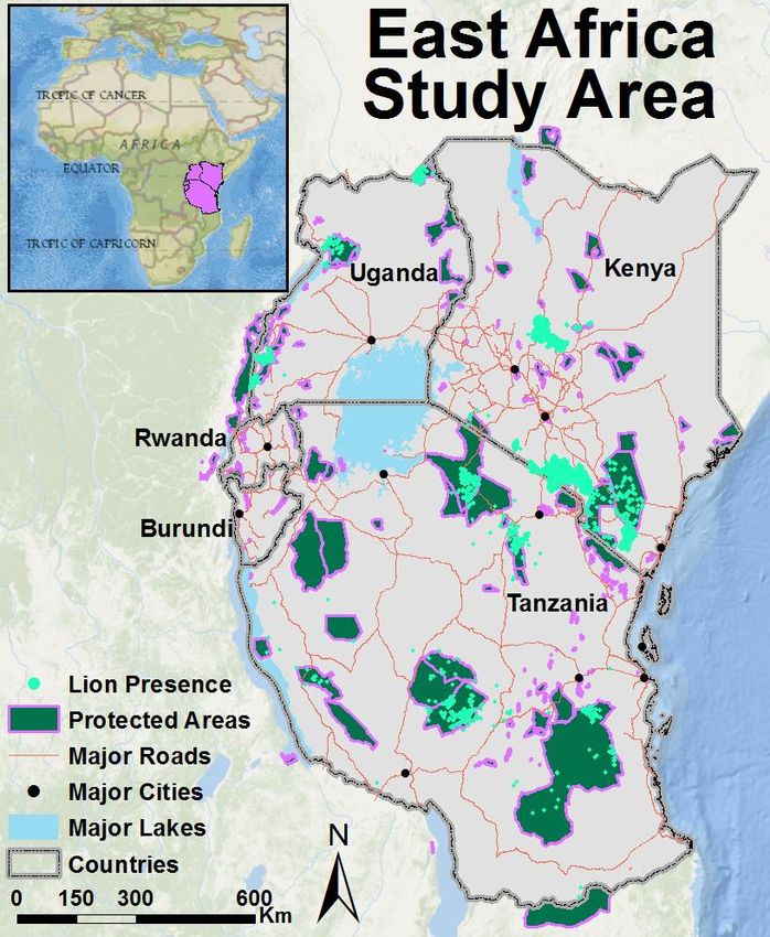
Abstract
Lion (Panthera leo) populations and habitat range are in steep decline. Lions are increasingly
isolated in protected areas and other pockets of habitat. Habitat fragmentation lowers effective
population size and increases vulnerability to threats such as inbreeding depression and localized
catastrophes. Conserving connecting habitat between lion populations is critical for mitigating
effects from fragmentation. With approximately half of all remaining lions and a rich network of
protected areas, the East African Community presents vital opportunities to preserve connectivity. I
collected 69,068 lion presence locations from field researchers and overlaid these locations with a
suite of environmental variables. Due to strong biases in the presence data, I used an intuitive
approach of creating a habitat envelope from observed presence data, and then identified
combinations of environmental conditions that are conducive to lion presence. By determining the
distribution of these environmental conditions, I predict areas with habitat through which lions can
disperse, though may not be resident. I then identify contiguous patches of connecting habitat that
link protected areas with documented lion populations. I find that while many protected areas
remain connected, Uganda’s lion populations in Murchison Falls and Queen Elizabeth National
Parks are critically isolated. Furthermore, my analysis suggests several bottlenecks and gaps that
constitute high priority areas for conserving or restoring connectivity.

                                                                                                      1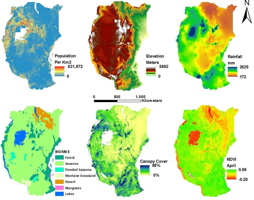
Contents
Abstract ......................................................................................................................................................... 1
Introduction .................................................................................................................................................. 4
   Connectivity Modelling ............................................................................................................................. 8
   Previous Studies ...................................................................................................................................... 10
   Study Area ............................................................................................................................................... 13
   Objectives ............................................................................................................................................... 16
Methods ...................................................................................................................................................... 17
   Data ......................................................................................................................................................... 17
       Presence Data ..................................................................................................................................... 17
       Environmental Data ............................................................................................................................ 18
       Vegetation........................................................................................................................................... 18
       Climate ................................................................................................................................................ 19
       Landscape features ............................................................................................................................. 21
       Human Population .............................................................................................................................. 21
       Sampling.............................................................................................................................................. 22
   Dispersal Habitat Analysis ....................................................................................................................... 22
       Annuli Formulation ............................................................................................................................. 23
       Exploratory Data Analysis ................................................................................................................... 26
       Habitat Envelope ................................................................................................................................. 27
       Paired Interactions .............................................................................................................................. 29
       Complex Interactions .......................................................................................................................... 31
       Refined Connecting Habitat ................................................................................................................ 31
Results ......................................................................................................................................................... 32
   Exploratory data analysis ........................................................................................................................ 32
       Woodland Model ................................................................................................................................ 35
   Envelope Model ...................................................................................................................................... 35
   Paired Interactions .................................................................................................................................. 40
   Complex Interactions .............................................................................................................................. 42
   Refined Model......................................................................................................................................... 46
   Improving the Model .............................................................................................................................. 56
   Applications............................................................................................................................................. 57

                                                                                                                                                                  2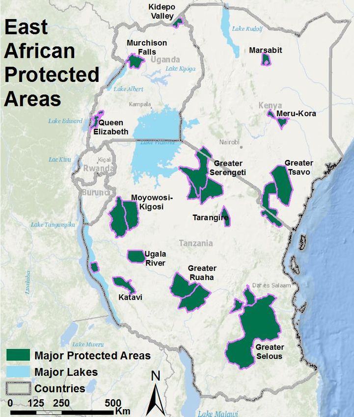
Acknowledgements..................................................................................................................................... 58
References .................................................................................................................................................. 59
Appendices.................................................................................................................................................. 66
   Appendix A: IUCN Classification of East African Protected Areas .......................................................... 66
   Appendix B: Lion Population Estimates: East Africa (excerpted from Bauer et al. 2005) ...................... 67
   Appendix C: Lion Presence Data Sources and Methods. ........................................................................ 68
   Appendix D: Correlations between environmental variables. ................................................................ 69
   Appendix E: Results of Woodland Model. .............................................................................................. 70
   Appendix F: Range of each variable in lion dispersal habitat envelope. ................................................ 71
   Appendix G: Annuli for each variable within the envelope of suitable dispersal habitat for lions. ....... 72

                                                                                                                                                              3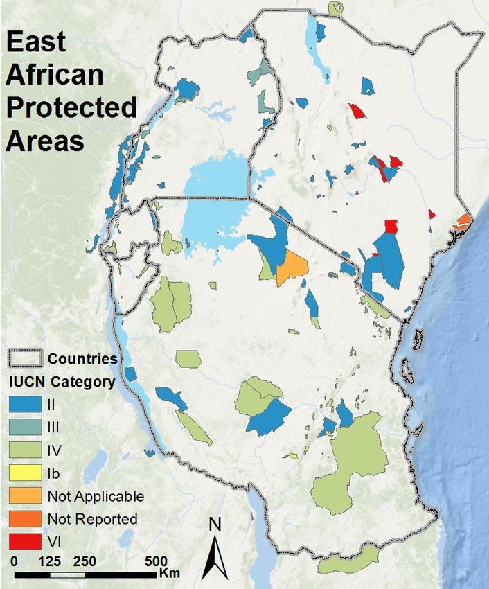
Introduction
Lion (Panthera leo) populations have declined precipitously in both size and extent, with losses
more severe than for other African carnivores (Patterson et al. 2004, Bauer et al. 2005, IUCN 2006).
Losses will continue (Riggio et al. 2013). Recent estimates suggest that approximately 35,000 lions
remain in Africa, but that lions currently occupy only 25% of their former range (Riggio et al. 2013).
In contrast to the current population, as many as 500,000 lions may have existed in 1950 (Myers
1975). As lions’ range shrinks, they face severe threats including loss of prey, habitat disturbance,
and conflict with humans (Nowell & Jackson 1996, Ray et al. 2005, IUCN 2006, Bauer 2008, Linnell
et al. 2008). People are the ultimate source of these threats. Furthermore, populations in protected
areas frequently suffer losses through edge effects when lions on the periphery of protected areas
come into conflict with adjacent human populations (Woodroffe & Ginsburg 1998). Several studies
find that human presence is a driving factor of lion decline and extinction. A rough estimate of
twenty-five people per km2 is the maximum human population density that resident lions can
tolerate (Woodroffe 2000, Loveridge & Canney 2009, Riggio et al. 2013). Protection of only a small
portion of lions’ range (Nowell & Jackson 1996, Crooks 2011) exacerbates threats to lions. Without
concerted conservation efforts, lions will go extinct or become extremely rare (Loveridge & Canney
2009).

Lions are a valuable species and a useful tool for the conservation of ecological communities. They
perform ecological functions that may benefit human communities (Ripple et al. 2014). As an apex
predator (Vanak et al 2013), lions play a critical ecological role (IUCN 2006, Sergio et al. 2008,
Ripple 2014), and their decline may result in trophic cascades that fundamentally alter
communities and reduce biodiversity (Crooks & Soule 1999, Ripple et al. 2014). One of the famed
“Big Five” African mammals, lions are a primary attraction of the tourism industry (Nowell &
Jackson 1996, Ray et al. 2005, IUCN 2006, Naidoo et al. 2011) and bring significant financial
benefits to countries and some local communities (Packer et al. 2009, Lindsey et al. 2007). Lions
contribute to the conservation of wild habitat that might otherwise be converted for human use
(Lindsey et al. 2012). As a habitat generalist (Nowell & Jackson 1996, Bauer et al. 2005), lions are an
effective conservation umbrella species (Carroll et al. 2001, Ray et al. 2005, Caro 2010, Caro &
Riggio 2013); their conservation benefits a host of other wildlife populations (Branton &
Richardson 2010). Carnivores are also good indicator species for studying habitat disturbance and
for conservation planning (Soule & Terborgh 1999, Morrison Et al. 2007). Thus lion declines have
significant repercussions for both ecological and human communities.

                                                                                                        4
As a result of population losses and anthropogenic threats, lions are becoming rare outside of
protected reserves and other fragments of suitable habitat (Woodroffe 2001, Ogada et al. 2003,
Patterson et al. 2004, Packer et al. 2005, Loveridge & Canney 2009, Mesochina 2010, Bauer et al
2012). The loss of habitat, both spatially and qualitatively, is the foremost threat to carnivores
(Crooks et al. 2011), and rapid human population growth and economic development in Africa lead
to higher anthropogenic pressure across lions’ range (Loveridge & Canney 2009). As a result,
despite the continent’s rich community of carnivores, connectivity for these populations is lower
than in other geographic regions (Crooks et al. 2011). Carnivores are more vulnerable to
fragmentation than other taxa, primarily because they live at lower densities than their prey
species (Noss et al. 1996, Woodroffe & Ginsberg 1998, Ceballos & Ehrlich 2002, Kissui 2008, Ripple
et al. 2014). Carnivores such as lions that are classified as Vulnerable to extinction (IUCN 2013)
suffer significantly higher rates of fragmentation than species of Least Concern (Crooks et al 2011),
strong evidence that connectivity is directly linked to lion conservation.
The area of a habitat patch and the severity of its isolation are primary factors affecting the
abundance of its carnivore populations (Crooks 2002). Furthermore, the habitat area needed to
sustain a particular abundance of a carnivore is related to the size of that carnivore (Crooks 2002).
Thus lions require larger habitat patches than some other African carnivores and are particularly at
risk from fragmentation (Crooks 2002). Local threats are not the only concern, as species with
fragmented ranges are more vulnerable to climate change and other range-wide transformations
(Heller & Zavalenta 2009).
Isolated lion populations pose serious conservation challenges. The smallest populations are most
vulnerable (Nowell & Jackson 1996). Isolation causes inbreeding depression and can reduce
fertility (Nowell & Jackson 1996, Frankham 2005), as occurred with lions in Ngorongoro Crater
(Packer et al. 1991, Ray et al. 2005). Fragmentation reduces lion abundance and effective
population size, and increases vulnerability to extinction (Nowell & Jackson 1996, Frankham 2005,
Hilty et al. 2006). Isolation may cause genetic drift (Soule & Mills 1998). In addition, marginal
populations may depend on immigrants from more productive source populations to maintain
stable numbers (Hanby et al. 1995). Without immigrants, these populations may not persist.
Genetic variation in lions shows that historically, populations were connected throughout Eastern
and Southern Africa (Dubach et al. 2013). Male lions always disperse from their natal prides and
female dispersal is a primary factor in population expansion (Dolrenry et al. 2014).
5Bjorklund (2003) found that lion populations require at least 50 prides to avoid inbreeding
depression, but that 100 prides are preferable. Inbreeding decreases survival and lowers fecundity.
The number of lions and the area necessary to sustain a minimal viable population changes in
response to wide variation in pride size (VanderWaal et al. 2009) and territory size (Bjorklund
2003). In terms of genetic stability, however, large prides are not a substitute for the space needed
to sustain 50 exclusive pride territories. Few reserves and national parks are sufficiently large to
sustain minimum viable populations (Nowell & Jackson 1996, Bjorklund 2003). In addition, lions
often depend on areas adjacent to reserves for additional resources (Kissui 2008). Africa suffers
high birth rates, rapid economic development, and extensive land conversion (Balmford et al. 2001,
Doos 2002). As a result, habitat on the periphery of protected areas is dwindling rapidly or has
already disappeared. Thus, when populations containing 50 prides are not feasible, it is imperative
that lions immigrate from other populations. Furthermore, Bjorklund (2003) found that a lack of
dispersal from natal prides leads to inbreeding, and so it is important for lions to emigrate out of
populations in addition to immigrating into them.
One method for mitigating habitat fragmentation for lions is to conserve connectivity between
populations (Brown & Kodric-Brown 1977, Hilty et al. 2006). Ecological connectivity is “the
movement of organisms or ecological processes across landscapes” (Crooks et al. 2011). A corridor
is a geographic area of habitat “in a dissimilar matrix, that connects two or more larger blocks of
habitat and that is proposed for conservation on the grounds that it will enhance or maintain the
viability of specific wildlife populations in the habitat blocks” (Beier & Noss 1998). It is critical that
a corridor provide a functional link between habitat patches, as opposed to just a theoretical link
(Crooks et al. 2012). Well-designed studies consistently find that corridors can reduce the impacts
of fragmentation (Brown & Kodric-Brown 1977, Beier & Noss 1998). More specifically, Norton et al.
(2010) found that naturally occurring corridors are more effective than human-created alternatives
and that designated corridors can increase movement between patches by 50%. Well-connected
landscapes can also influence meta-population dynamics through mechanisms such as a rescue
effect, whereby immigrants contribute demographically and genetically to a population (Brown &
Kodric-Brown 1977, Packer et al. 1991). The rescue effect increases population resiliency
(Loveridge & Canney 2009) and decreases the risk of a population going extinct (Nowell & Jackson
1996).
Connectivity is essential for lion conservation (Dubach et al. 2013). Dolrenry et al. (2014) modelled
the effects of connectivity between several lion populations in East Africa and found that male lions
6can disperse at large distances while females exhibit shorter dispersal, but are requisite for
recolonizing habitat patches. Connectivity has enabled lions to recolonize areas (Dolrenry et al.
2014) and subsidize marginal populations (Hanby et al. 1995). However, while numerous studies
have geographically mapped the resident range of lions, thus far no one has mapped, at a regional
scale, the distribution of habitat that may not sustain resident lion populations but can act as
corridors linking populations. Mesochina et al. (2013) found that lions use a significant portion of
their range through Tanzania only temporarily, which confirms lions’ movement through non-
resident areas. Large carnivores have also demonstrated an ability to tolerate high human
population density under certain conditions (Athrey et al. 2013, Linnell et al. 2001). Ascertaining
those conditions is critical to distinguishing between resident habitat and dispersal habitat.
Lions are well-studied, but research has been biased towards populations in protected areas (Bauer
et al. 2005, Loveridge & Canney 2009). Our knowledge of lion distribution and behavior outside
reserves, particularly in areas with high human impacts, is deficient (Chardonnet 2002, Van Dyck &
Baguette 2005, IUCN 2006, Dolrenry 2013). Yet one-third of lions live outside of reserves (Riggio et
al. 2013). In order to develop conservation strategies for maintaining connectivity, it is critical that
we improve our understanding of dispersal habitat that may function as corridors (Dubach et al.
2013). Vanak et al. (2013) found that dispersing lions broaden their diet from the species’ main
prey base, and that prey availability is a factor in lion movement. That study also found that lions
demonstrate a preference for thick riverine vegetation during the dry season and that they tended
to avoid woodland and open scrub. Several studies found that lions in pastoral lands were less
active during daylight than lions in neighboring reserves with similar habitat, and that lions in
human-dominated landscapes alter their feeding behavior (Maddox 2003, Mogensen 2011).
Similarly, Mogensen et al. (2011) found that lions in pastoral lands acted more like reserve lions
during periods of high vegetation growth. These findings suggest that dispersing lions adapt to
their circumstances. Assumptions about lion foraging from resident populations may not apply to
dispersing individuals.
Research on other large carnivores corroborates the notion that lions dispersing outside of
protected areas may act differently than lions in ideal habitat. Dickson et al. (2005) tracked cougars
and found that they moved through riparian vegetation more than grassland, woodland, or desert
habitat. The cougars moved rapidly through human-dominated areas. In India, a population of
leopards exists in areas with 300 people per km2 by adapting their diet; other carnivores also
inhabit the same landscape matrix of agricultural lands and wild habitat (Athreya et al. 2013).
7Atypical populations such as these leopards provide a compelling argument for approaching
conservation at the landscape level rather than managing protected areas in isolation (Athreya et al.
2013). In the absence of persistent and ubiquitous persecution, carnivores are very adaptable and
can survive in situations previously thought intolerable.
Management practices further complicate strategies for conserving carnivore habitat and
connectivity. Linnell et al. (2001) found that North American carnivore density can increase in
areas of growing human population if land use policies are well-designed. Their research found no
direct correlation between carnivore and human abundance. Their findings suggest that population
density thresholds are not absolute, but depend on other factors such as how humans use the
landscape.
It is clear from this body of literature that lions and other carnivores demonstrate tendencies in
their movement patterns and some of these tendencies relate to combinations of factors, rather
than individual variables. For example, estimates of human density thresholds that preclude
resident lion populations are useful for management, but do not necessarily account for individuals
moving rapidly through an area. Other factors likely influence the relationship between lions and
human population density (Loveridge & Canney 2009).
Lion connectivity studies are further limited by insufficient data to determine maximum dispersal
distances for individuals, though males can likely emigrate to populations more than 300 km
distant from the source (Dolrenry et al. 2014). However, even 300 km may not be their maximum
dispersal distance. Tigers can emigrate up to 650 km (Joshi et al. 2013).
Connectivity Modelling
Numerous studies have sought to model connectivity for large carnivores and other taxa.
Conventional models have two components: habitat suitability modelling and corridor modelling.
Studies typically estimate habitat suitability from statistical models or from expert opinion
(Rabinowitz & Zeller 2010, Kertson et al. 2011, Poor et al. 2012). The second step predicts which
areas in the landscape function as corridors based on paths through suitable habitat. Many analyses
depend on models that identify corridors based on routes of minimum cost-distance or routes
predicted based on electrical circuit theory (Poor et al. 2012). However, these models are poor
predictors of actual animal movement (LaPoint et al. 2013). Customized stochastic movement
models, an alternative approach, incorporate variation and individual decision-making in
8dispersing animals (Gardner & Gustafson 2004). But they require prodigious data to parameterize
correctly, which are particularly difficult to obtain for rare carnivores.
Probability models of suitable habitat assume that dispersing animals act according to conditions
where the species is most abundant. Dispersal habitat is not the same as resident habitat, but
connectivity models derived from species distribution models do not recognize the distinction
(Carroll et al. 2011). Connectivity analyses based on distribution models are therefore likely to
under-predict movement potential, especially in landscapes where conditions outside of protected
areas may be widely different from conditions in protected areas. This issue is especially relevant to
my research, which incorporates presence-only data primarily from clusters of unrepresentative
research areas. Few statistical models are suitable for the presence-only data I collected. Many
statistical models also assume linearity in relationships between predictor and response variables.
However, linearity rarely represents ecological reality (Loveridge & Canney 2009).
Constraints in the data further limit my analysis. With a large study area and a fairly coarse grain
size for connectivity modelling, the environmental datasets used for this analysis contain error and
may not represent fine-scale patterns in lion movement. Statistical models also assume unbiased
input data. However, the presence data I collected exhibit clear biases. There were no consistent
sampling protocols and research areas reflect sites of ongoing lion research, namely in areas where
lions are most common. The data are clustered in the areas where researchers work and, therefore,
are spatially autocorrelated. Without consistent data on dates of samples, I was unable to account
for temporal autocorrelation in the data as well.
With a primary interest in the behavior of lions away from lion population centers and aware of the
constraints of the presence data, I eschewed statistical approaches in favor of a model that
identifies all ecological conditions in which lion presence is recorded, rather than the most
probable conditions. By identifying where similar ecological conditions occur across the landscape,
I can predict all areas where we would expect lions to occur, even if only temporarily. This focus on
all habitats that lions use, as opposed to habitats where lions are most abundant, is a fundamental
advantage in predicting dispersal habitat.
Annuli – concentric, exclusive distance classes – present an intuitive method for parsing the
landscape and examining environmental conditions in which lions occur. Many ecological analyses
incorporate distance classes, such as tests of autocorrelation (Diniz-Filho et al. 2003), and annuli
9have been used to spatially compare occurrence rates of ecological phenomena (Nakamura et al.
1997, Santos & Tabarelli 2002, Joppa et al 2008, van Noordwijk 2011).
The most important constraints to my analysis are sampling biases in the lion presence data and
error in interpolated (rainfall), remotely sensed (vegetation indices, elevation), and modelled
(population density) datasets. Distance classes, whether geographic or distributional, control for
this error and accurately represent the precision of my analysis. Given the presence-only nature of
the lion occurrence data, distance classes create clear, understandable buffers around observed
occurrence that can capture some areas of false-absence in the occurrence dataset and imprecision
in environmental datasets.
Previous Studies
This paper builds off a foundation of research that explores habitat distribution and connectivity for
lions, and connectivity more broadly in East Africa. Most recently, Dolrenry et al. (2014) used
incidence function models to predict the dispersal of lions between major populations. They
analyzed how dispersal affects population demographics, but did not spatially predict where lions
move through the landscape that separates resident habitat patches. Instead, the authors used data
collected from dispersing lions to predict average and maximum dispersal distances for male and
female lions. Their models further constrain connectivity based on patch size and spatially explicit
human density data. Their research reveals significant differences between male and female
dispersal: male lions disperse further and “rescue” populations regularly, whereas female lions
disperse shorter distances but have a greater colonizing effect than males. Crucially, the authors
note the importance of lion survival during dispersion and that even large populations still require
dispersal to remain viable.
Jones et al. (2009) took a different approach to connectivity by evaluating individual wildlife
corridors throughout Tanzania. They gathered expert knowledge to classify corridors’ status and
estimate the scope and severity of threats to each corridor. The paper describes 31 separate
corridors that link protected areas. The authors concluded that Tanzania’s wildlife corridors are
critically threatened, with most likely to disappear by the end of this year. The principle threats to
connectivity, the study finds, are land conversion, the bushmeat trade, and extractive industries.
Other studies take a broader view, modelling the distribution of lions throughout Africa. Loveridge
and Canney (2009) mapped the distribution of lions using two methods to estimate the extent of
lions’ range and their density across that range. The first method predicts lion density in response
10to data on prey density and its correlates, rainfall and soil nutrients. The second model applies
statistical hurdle models that predict presence or absence and estimate population density, and
then combine the two outputs to estimate abundance. Both parts of the hurdle model regress lion
data against a suite of environmental variables. The authors conclude that in some areas, their
models over-predict lion abundance, but in others, such as the Selous-Niassa ecosystem, the models
are highly representative.
Similarly, Celesia et al. (2009) modelled lion distribution and density throughout Africa in relation
to climactic factors, biotic variables, and landscape features. Like Loveridge and Canney, they used
regressions to relate lion data to environmental variables, but they acquired all of their lion data
from just 21 protected populations. The authors applied hierarchical partitioning to determine the
individual importance of each predictor variable independently. They found that climactic factors
explain most of the variation in lion distribution and density, while landscape features explain
approximately another third.
The latter two studies are critical to our knowledge of where lions occur and what conditions
constitute resident habitat, but they are less effective at predicting dispersal habitat. The former
two studies inform our understanding of the role connectivity plays in lion population dynamics
and where wildlife corridors occur in a large portion of the study area. However, neither explicitly
identifies dispersal habitat specifically for lions that links resident populations. This paper applies
a regional analysis that bridges the gap in scale between the continental distribution models and
the national and transnational connectivity studies. It also seeks to link the mapping component of
the Tanzanian wildlife corridors with the meta-population dynamics that Dolrenry et al. describe.
These goals reflect the work of Rabinowitz and Zeller (2010) to map corridors for jaguars
throughout their range in the Americas. Their research was founded on similar principles as this
study: fragmented populations, high vulnerability to isolation, a need for connectivity to mitigate
these threats, and a desire to inform regional conservation strategies. However, Rabinowitz and
Zeller base their analysis on expert opinion rather than biological data, and rely on simplistic least-
cost paths to predict habitat. This paper, on the other hand, takes an approach rooted in biological
data. It improves on statistical models because it does not emphasize resident habitat over
dispersal habitat.
11Figure 1: Map of the East African Community study area and recorded lion occurrence.
12Study Area
The five countries of the East African Community (henceforth East Africa) cover more than 1.7
million km2 of land (28.86o – 41.89o E, 11.75o S – 4.63o N) from the Great Lakes region of central
Africa to the continent’s east coast (Figure 1). The five countries have a combined human
population of 154.3 million people ranging from 10 million in Burundi to 46.6 million in Tanzania.
The region is characterized by high population growth rates ranging from 2.1% – 3.3%, and a total
population density of approximately 90 people per km2 (CIA 2014). However, while several large
population centers (e.g. Nairobi, Dar Es Salaam, Kampala, Lake Victoria) are spread across the
region, much of the landscape has minimal human presence. Human population is dense in the
smaller countries in the west and around Lake Victoria, and less dense in Kenya and Tanzania,
particularly in areas of low rainfall, such as northern Kenya and rain shadows west of mountain
ranges.
Figure 2: Environmental characteristics of East Africa.
13The landscape ranges in elevation from sea level along the coast to 5882 m at the top of Mt.
Kilimanjaro (Jarvis et al. 2008, Figure 2). The vast majority of the region lies above 500 m. Annual
total rainfall (172 – 2625 mm) is lowest in the arid Somali region of the northeast and greatest
around Lake Victoria and on the mountains of northern Tanzania and Kenya (Hijmans et al. 2005).
The region experiences bimodal rainfall (Bradfield & DeWitt 2012), with most precipitation
occurring in October – December and March – May (Gelorini & Verschuren 2013). However, rainfall
patterns vary widely both regionally and temporally based on climate systems such as the
Intertropical Convergence Zone and the el Nino-Southern Oscillation (Gelorini & Verschuren 2013).
Recent years suggest significant declines in rainfall during the March – May period (Bradfield &
DeWitt 2012), which creates uncertainty about the effects of climate change on the region.
East Africa includes seven biomes, but is particularly renowned for three. It consists primarily of
Tropical and Subtropical Grasslands, Savannas, and Shrublands (Olson et al. 2004). Arid savannas
occur in areas with less than 820 mm of annual rainfall and moist savanna occurs in areas with at
least 1000 mm annually (East 1984). In a transition zone in central Tanzania, the savanna gives way
to miombo woodland landscapes that dominate southern Tanzania. While most of the landscape
has less than 20% canopy cover, patches of ecologically diverse montane rainforest occur across
East African mountain ranges. The eastern arc mountains stretching from southeastern Kenya to
east-central Tanzania exhibit the world’s highest rates of endemic plants and vertebrates per unit
area (Myers et al. 2000).
East Africa hosts numerous protected areas ranging in size from the 48,000 km2 Selous Game
Reserve to many smaller national parks, wildlife reserves, forest reserves, and community reserves
(IUCN & UNEP 2009, Figure 3, Appendix A). Several ecosystems, all with contiguous networks of
national parks and reserves, host lion populations with more than 500 individuals, in particular the
greater Serengeti, Selous, Ruaha, and Tsavo ecosystems (Bauer & Van Der Merwe 2004, Riggio et al.
2013).
Historically, lions have been widespread across East Africa (Bauer and Van Der Merwe 2004).
Largely as a result of the population centers in its large protected areas, East Africa holds
approximately half of all lions (Mesochina 2010, Riggio et al. 2013), with estimates of total lion
populations ranging from 7,199 – 22,335 individuals (Buaer et al. 2005, Appendix B). Bauer & Van
Der Merwe (2004) inventoried known populations and estimated 11,000 individuals. East African
populations exhibit the least genetic distance of all regional populations (Dubach et al. 2013), which
14suggests that its populations have been well-connected. Research from Kenya and Tanzania,
however, shows that lion dispersal is currently limited (Dolrenry et al. 2014). Jones et al. (2009)
found that a majority of corridors in Tanzania were critically threatened and unlikely to persist
after five years because of habitat loss. Thus, the historical links between populations are in dire
jeopardy.
I designated the spatial extent of the study area by including the entire administrative areas of the
five countries and excluding regions classified as lake ecoregions (Olson et al. 2004). I did not
include islands in the Indian Ocean or lakes in any analyses.
Figure 3: Major protected areas of East Africa
15Objectives
With approximately 50% of all lions (Mesochina 2010), extensive lion research (Bauer et al. 2005,
Dolrenry et al. 2014), a rich network of protected areas, and high variation in ecological conditions
and human impacts, the five countries of the East African community—Burundi, Kenya, Rwanda,
Tanzania, and Uganda—present many of the best and most pressing opportunities for conserving
connections between populations. Their shared political institutions and cultural history are
conducive to transnational conservation projects.
This paper is concerned specifically with the movement of individual lions and their genes across
their range. This research is intended to guide conservation planning and help researchers
prioritize areas of concern. I aim to accomplish three objectives that will enable conservation of
dispersal habitat, and thus preserve lion connectivity, across East Africa: 1) identify geographic
areas that are suitable for lion dispersal, 2) identify priority areas for connectivity, and 3) identify
populations that have the highest risk of isolation.
To accomplish these objectives I analyze 69,068 lion presence points that I acquired from 16 field
research teams and relate lion presence to a suite of environmental variables. My analysis focuses
on where lions are capable of occurring (i.e. habitat conducive to dispersal) rather than areas
where lions are resident or most common. I use an intuitive approach of creating a habitat envelope
and then use annuli to examine the interactions of variables to predict conditions that are
compatible with lion dispersal, even if they are not compatible with permanent habitation. Within
the broader context of my objectives, I seek to answer the following research questions:
1) Which variables most strongly influence lion presence?
2) What environmental factors influence lion tolerance of human presence?
3) In what combinations of variables do lions occur and where in East Africa do those
combinations occur?
4) How do areas with these environmental conditions spatially relate to existing
populations of lions, and which patches of dispersal habitat intersect two or more
protected areas with lion populations?
5) Which areas of dispersal habitat are most critical to preserving connections between
lion populations?
6) Where do gaps occur between patches of dispersal habitat that constitute prime targets
for restoring connectivity?
167) Which existing lion populations are most isolated from other populations, and thus
most in need of active management to ensure the long-term viability of lions?
Methods
Data
I conducted all data processing using ArcGIS 10.2 (Esri 2013). With the exception of input datasets,
I performed all analyses using a 500 m grain size.
Presence Data
I collected 69,085 lion presence data from 17 researchers or research teams working in Kenya,
Tanzania, or Uganda (Appendix C). Communication with researchers revealed no contemporary
presence data for lions in Burundi or Rwanda.
Researchers’ methods for data collection included telemetry data, sightings, spoor counts, and
confirmed incidences of lion-human conflict. Some researchers provided occurrence data as GPS
coordinates using a variety of coordinate systems, all of which I reprojected into WGS 1984
geographic coordinates. For researchers who listed a distance to sighting, I excluded points with a
distance greater than 250 m, one-half of the grain size of my analysis. Other researchers provided
grid cells with confirmed lion presence, primarily from telemetry data; this method was used to
protect original data. All such grid datasets had a grain of 250 m or smaller. I converted the
presence cells to centroids referenced to the WGS 1984 datum. Few researchers provided data on
date, time, or number of individuals for their data. Data points were collected from 2004 – 2013.
I then aggregated all 69,085 lion point locations and reprojected them into the WGS 1984 Africa
Albers Equal Area Conic coordinate system. I used this coordinate system for all subsequent
analyses. I removed 17 locations that were clearly inaccurate, such as a point off the coast of
Tanzania, a point in the middle of Lake Turkana, Kenya, and several points just outside national
borders, and thus outside the study area. The final dataset of lion presence consisted of 69,068
locations (Figure 1).
I randomly assigned 90% (62,160) of the points as training data and the remaining 10% (6,908) of
points as test data to validate the model.
I created a stratified random sample of 10,000 pseudo-absence or background data points to
compare environmental conditions across the landscape with conditions at the lion presence
locations. I stratified the background points by WWF ecoregion (Olson et al. 2004), weighted by
17ecoregion area. I selected a stratified random sample in order to ensure that the background points
captured the full variation of environmental conditions across the landscape.
Environmental Data
I selected environmental variables based on a review of the literature and publicly available
datasets for the study area. Such studies form a consensus around including both ecological and
anthropogenic predictor variables. Rabinowitz & Zeller (2010), considered vegetation cover,
human population density, elevation, distance to roads, and distance from settlements in their
study of Jaguar connectivity throughout the Americas. Loveridge and Canney (2009), modelled the
distribution of lions across Africa in relation to precipitation, vegetation cover (NDVI), soils,
livestock density, a human footprint dataset, temperature, protected areas, and human population
density, and found that mean NDVI is a good predictor of lion residency. Kissui et al. (2010) found
that cub production is higher near rivers and in thick vegetation, but that distance from roads has
no impact. Similarly, Joshi et al. (2013) studied connectivity for tigers and found that human
settlements and road density impact movement, but distance to roads does not.
For this report, I considered 15 variables (Table 1): human population density at three scales,
distance to dense human populations, distance to rivers, distance to lakes, distance to major roads,
distance to protected areas, April NDVI, August NDVI, percent canopy cover, total annual rainfall,
dry-season (June – October) rainfall, elevation, and slope. I did not include land use data because
national data sets are incompatible and because conventional global land use and land cover
datasets are poor predictors of mixed savanna and agricultural landscapes (Riggio et al. 2013).
All environmental datasets were reprojected into the WGS 1984 Africa Albers Equal Area Conic
coordinate system. Whenever possible, I collected data for an area that extended to a 20 km buffer
around the study area to account for influence of environmental factors along the borders of East
Africa. All input datasets were processed at 500 m resolution using a snap raster such that grids for
each variable aligned.
Vegetation
A review of the literature suggests that vegetation quantity and structure affects large carnivore
behavior and movement (East 1984, Hayward et al. 2007, Loveridge & Canney 2009, Rabinowitz &
Zeller 2010, Joshi et al. 2013, Loarie et al. 2013).
The Normalized Difference Vegetation Index (Rouse et al. 1973) is a measure of vegetation
abundance derived from remote sensing data. NDVI relates to a wide range of ecological processes
18(Pettorelli et al. 2005), including wildlife distribution and behavior (Pettorelli et al. 2011). Above-
ground vegetation correlates with herbivore abundance in Africa (Coe et al 1976), which represents
prey availability for lions (Loveridge & Canney 2009). Prey abundance, in turn, is the primary factor
in a habitat’s carrying capacity for carnivores, explaining approximately 60% of the variation
(Hayward et al. 2007). Vegetation also influences hunting behavior, with males typically hunting in
areas with shorter line-of-sight than where they rest (Loarie et al. 2013). Several studies include
NDVI as a predictor variable when modelling distribution of lions (Loveridge & Canney 2009), or
connectivity for other large carnivores (Joshi et al. 2013).
NDVI data were collected from NASA’s MODIS MOD13Q1 16-day composite global dataset of
vegetation indices, with a resolution of 230 m (Huete et al. 2002). I acquired scenes during the
rainy season sampled April 22 – May 7 and during the dry season, sampled August 12 – August 27.
For each season, I mosaicked seven scenes that covered the entire study area for each of the last
five years for which data were available, 2008 – 2012. The MOD13Q1 dataset includes a pixel
reliability layer. I masked out pixels classified as No Data, Snow/Ice, and Cloudy. I calculated 2008 –
2012 average NDVI for each sampling period, including only values of suitable reliability.
Vegetation Continuous Fields, also known as percent canopy cover, is available from NASA’s MODIS
MOD44B annual dataset at 230 m resolution (Hansen et al. 2002), with sampling beginning and
ending in March. The most recent available datasets are for 2010 – 2011, and so I mosaicked the
seven scenes covering the study area for each year with the sampling period beginning in 2008 –
2010 and calculated average canopy cover from those datasets.
Climate
Studies show that climatic factors correlate with lion distribution (Celesia et al. 2009, Loveridge &
Canney 2009). Rainfall also correlates with African herbivore abundance (East 1984). Celesia et al.
(2009) found that temperature and precipitation collectively explain 62% of the variation in lion
demographics across its global range. This report, however, treats elevation as a substitute for
temperature, as temperature does not fluctuate across the study area at the same scale as discussed
in Celesia et al. Precipitation is a reliable predictor of habitat for lions, particularly through its
correlation with herbivore density (Coe et al. 1976, East 1984). Precipitation explains 28% of the
variation in lion demographics across their range (Celesia et al. 2009), and 70% of the variation in
prey biomass, which in turn shows a correlation with lion abundance of 0.92 (Loveridge & Canney
2009).
19Table 1: Summary of sources and processing steps for environmental datasets.
Variable Source Pre-processing
Vegetation Averaged monthly NDVI values (230 m pixels) over five years (2008 -
MODIS NDVI
Index 2013) after removing low-quality pixels from each dataset.
Canopy Averaged annual percent canopy cover (230 m pixels) over the three
MODIS VCF
Cover most recent years for which data are available (2008-2010)
Collected average monthly precipitation under current conditions. I
summed all twelve months and resampled to 500 m pixels to estimate
Rainfall WorldClim
total annual rainfall. I also summed the months of June - October and
resampled to 500 m to estimate dry season rainfall.
Collected from USGS at 250 m resolution. I did not perform pre-
Elevation SRTM
processing.
Slope SRTM I calculated slope from the SRTM elevation dataset.
I selected pixels classified as "lakes" or "reservoirs" and calculated the
Lakes WWF GLWD-3
distance to these areas for each 500 m pixel in the study area.
I collected the GLWD-3 flow accumulation data and manually applied
a threshold of at least 1,000 accumulated pixels to designate rivers. I
Rivers WWF GLWD-3
based this threshold on manual comparison of flow accumulation with
rivers evident from satellite imagery.
WWF I designated ecoregions by the WWF Eco-Number. I excluded the
Ecoregion
Ecoregions "lakes" ecoregion from the study area.
I selected primary and tarmac roads from the Tracks4Africa dataset
Roads Tracks4Africa and calculated the distance from roads for each 500 m pixel in the
study area.
Protected I selected all protected areas within 20 km of East Africa with an IUCN
WDPA
Areas classification. I also included the Ngorongoro Conservation Area.
Human I calculated people per km2 at spatial scales of 1 ha, 1 km focal radius,
AfriPop
Density and 5 km focal radius.
I set 228 people per km2 as the maximum tolerated human density
Distance
and the threshold for high population density (Table 3). I calculated
to Human AfriPop
the distance to areas of high human population density for each 500 m
Population
pixel in the study area.
I collected current monthly rainfall data from Worldclim (Hijmans et al. 2005), a global interpolated
dataset, at 30 arc-second (~1 km) resolution. I resampled to 500 m resolution. I summed monthly
average to determine annual rainfall, and summed average rainfall for the months of June – October
to determine dry-season rainfall.
I collected elevation data from the USGS Shuttle Radar Topography Mission (Jarvis et al. 2008) at
250 m resolution.
20Landscape features
I acquired spatial and qualitative data on protected areas from the World Database of Protected
Areas (IUCN & UNEP 2009) and subset the database to include only protected areas within East
Africa or its 20 km buffer. I calculated distance from protected areas for a 500 m raster dataset.
I derived slope from the SRTM dataset at 250 m resolution.
I derived rivers from the WWF HydroSHEDS dataset (Lehner et al. 2006). The HydroSHEDS stream
network is based on flow accumulation, and does not precisely match the location of rivers. I
manually compared flow accumulation from the HydroSHEDS stream network to satellite imagery
and established a threshold of 1,000 accumulated cells as an indicator of actual stream presence. I
subset the stream network to only include features with a flow accumulation above this threshold,
and calculated distance from streams across the entire study area for a 500 m raster dataset.
I derived distance from lakes for a 500 m raster dataset from the WWF Global Lakes and Wetlands
Database Level 3 dataset (Lehner & Doell 2004), which I subset to include only water bodies
designated as lakes or reservoirs.
I derived major roads from the Tracks4Africa Enterprises road dataset (Tracks4Africa 2010),
subset to include types 1 – 6 (highways and main roads) and 11 (secondary tar roads).
Human Population
I collected data on human population density from the AfriPop Alpha version 2010 (Linard et al.
2012) estimates of people per 1 ha grid square for each of the five countries in the study area. I
multiplied cell values by 100 in order to represent the values in terms of people per km2. I
calculated the mean population density within a 1 km radius and a 5 km radius in order to test the
effects of human presence at varying scales, while also retaining the original 1 ha scale. I therefore
incorporate three measures of population density into the analysis.
I created a distance to settlement dataset by identifying a threshold for high human population
density (see results), and then calculating the distance to areas of high population density for a 500
m raster dataset. I did not use a settlement layer because I did not have a dataset consistent across
the study area at the scale of this analysis. Population at the one-hectare scale of the AfriPop
dataset, however, provides a fine-scale metric of high-impacted areas that I can relate directly to
the occurrence of lions across the landscape.
21Other studies have included variables such as livestock density, land use, and land cover. For many
variables, I determined that data quality was insufficient (e.g. land cover, Riggio et al. 2013), or
datasets were inconsistent or incomplete for the study area (land use).
I considered including density variables for roads and rivers. I decided, however, that these
datasets contain too much uncertainty. In particular, I lacked confidence in distinguishing road
characteristics such as number of vehicles per day. This factor is potentially critical as some minor
roads may facilitate lion movement, while others may hinder it (Zeke Davidson, personal
communication, October 9, 2013).
Sampling
I sampled each environmental dataset at each presence location within the training dataset, and at
a composite dataset of all training data and background points. In all cases, I performed sampling
using bilinear interpolation because the lion presence locations lack precision. Bilinear
interpolation samples the eight cells surrounding each point. It assigns a value to each point based
on the weighted average of the surrounding cells, with the closest cells having the greatest
influence. Bilinear interpolation accounts for the fact that points occurring on the periphery of a cell
may represent a lion occurrence that actually was located in an adjacent cell.
Dispersal Habitat Analysis
I analyze habitat conducive to lion dispersal by applying several successive methods that
repeatedly refine predictions of suitable habitat (Figure 4). Each step is critical to providing a more
restricted study area for subsequent steps. I process suitable habitat in five steps: 1) explore data to
identify significant relationships between environmental factors and lion occurrence, 2) create an
envelope model to constrain the relevant landscape, 3) analyze paired interactions of
environmental annuli, 4) analyze complex annuli interactions between sets of variables, and 5)
identify habitat patches that connect lion populations in protected areas.
22Presence Data Environmental
Data
Envelope Paired Complex
Model Interactions Interactions
Refined
Habitat Model
Validation
& Conclusions
Figure 4: Flowchart of habitat analysis methods.
Annuli Formulation
I separated variables into two categories: localized and non-localized. Localized variables refer to
landscape features that are present in certain locations and absent elsewhere. Where the feature is
absent, the landscape is classified by the distance of each pixel to the nearest feature. This category
includes protected areas, roads, rivers, lakes, and areas of high human density. Non-localized
variables refer to variables for which every pixel in the study area has a value that represents a
quantity or metric of that variable. Non-localized variables include all vegetation indices, rainfall,
elevation, slope, and human population density.
For localized features, I applied annuli at 10 km intervals up to a maximum of 50 km (Joppa et al.
2009), with a final class encompassing all areas beyond 50 km (Figure 5). Thus I had seven classes,
0, 0 – 10, 10 – 20, 20 – 30, 30 – 40, 40 – 50, and greater than 50 km from the nearest feature. For
features represented as lines – rivers and roads – a value of 0 represents all areas within 1 km of
the nearest feature. A value of 0 – 10 represents areas 1 – 10 km from the nearest feature.
23For non-localized variables, I apply annuli in distributional space using intervals of 0.5 standard
deviations above and below the mean (Figure 6). Because the variable values are not normally
distributed, this interval was necessary to parse data with heavily skewed or leptokurtic
distributions.
Figure 5: Annuli representing 10 km distance intervals from protected areas in East Africa.
242
Figure 6: Distributional annuli for mean people per km within a 1 km radius of each 500m cell. Each class represents the
2 2
number of one-half standard deviations (9 people per km ) above or below the mean population density (12 people per km )
at lion occurrence locations. Annulus 8 includes all areas above the 99.9% threshold for tolerable population density.
Ecological relationships between lions and predictor variables change over large geographic scales
(Loveridge & Canney 2009) such as my study area. Most of the lion presence locations come from
study sites in semi-arid open grasslands of Kenya, rather than the miombo woodland or forest
ecosystems of southern Tanzania (where the Selous ecosystem is suspected to harbor the largest
single lion population worldwide) and western East Africa. I therefore tested two models. The first
model treated the entire study area as a single unit; the second divided the study area into two
regions based on classifications from Nangendo et al. (2007, Figure 7): open grassland landscapes
(canopy cover less than 10%) and wooded landscapes (canopy cover greater than 10%). I classified
each pixel as either above or below the 10% threshold, and then reclassified each cell based on
whether the majority of the landscape within an 8.5 km radius was open or wooded. I selected the
227 km2 focal area as the median home range size observed in East African lion populations
25(Celesia et al. 2009). I ran identical analyses for both the unified and divided models to predict
dispersal habitat.
Figure 7: Grassland/Woodland zones for two-part model.
Exploratory Data Analysis
I performed exploratory data analysis in R x64 2.15.2 statistics software (R Core Development
Team 2012) using the ecodist package (Goslee & Urban 2007). I tested each environmental dataset
for a significant (α = 0.05) correlation with presence – pseudo-absence locations and with each
other dataset. I set 0.7 as a correlation coefficient threshold above which I would consider
environmental variables strongly correlated. However, because I do not apply statistical models, I
did not exclude strongly correlated variables from further analysis. The purpose was instead to
determine how much variation across the landscape this suite of variables captures.
26You can also read