The SPHERE infrared survey for exoplanets (SHINE) - arXiv
←
→
Page content transcription
If your browser does not render page correctly, please read the page content below
Astronomy & Astrophysics manuscript no. paperF100IIfinalb                                                                           ©ESO 2021
                                              March 9, 2021

                                                              The SPHERE infrared survey for exoplanets (SHINE)
                                                   II. Observations, Data reduction and analysis, Detection performances and
                                                                                  early-results
                                              M. Langlois1, 2 , R. Gratton3 , A.-M. Lagrange4, 5 , P. Delorme4 , A. Boccaletti5 , M. Bonnefoy4 , A.-L. Maire7, 6 , D. Mesa3 ,
                                                 G. Chauvin4, 20 , S. Desidera3 , A. Vigan2 , A. Cheetham8 , J. Hagelberg8 , M. Feldt6 , M. Meyer9, 10 , P. Rubini, H. Le
                                              Coroller2 , F. Cantalloube6 , B. Biller6, 12, 13 , M. Bonavita11 , T. Bhowmik5 , W. Brandner6 , S. Daemgen10 , V. D’Orazi3 , O.
                                              Flasseur1 , C. Fontanive13 ,3 , R. Galicher5 , J. Girard4 , P. Janin-Potiron5 , M. Janson28 ,6 , M. Keppler6 , T. Kopytova6 ,30 ,29 ,
                                              E. Lagadec14 , J. Lannier4 , C. Lazzoni27 , R. Ligi14 , N. Meunier4 , A. Perreti8 , C. Perrot5 ,24 ,25 , L. Rodet4 , C. Romero4 ,16 ,
                                              D. Rouan5 , M. Samland28 ,6 , G. Salter2 , E. Sissa3 , T. Schmidt5 , A. Zurlo17, 18, 2 , D. Mouillet4 , L. Denis26 , E. Thiébaut1 ,
arXiv:2103.03976v1 [astro-ph.EP] 5 Mar 2021

                                                  J. Milli4 , Z. Wahhaj16 , J.-L. Beuzit2 , C. Dominik19 , Th. Henning6 , F. Ménard4 , A. Müller6 , H.M. Schmid10 , M.
                                                     Turatto3 , S. Udry8 , L. Abe14 , J. Antichi3 , F. Allard1 A. Baruffolo3 , P. Baudoz5 , J. Baudrand5 , A. Bazzon10 ,
                                                    P. Blanchard2 , M. Carbillet14 , M. Carle2 , E. Cascone3 , J. Charton4 , R. Claudi3 , A. Costille2 , V. De Caprio23 ,
                                                  A. Delboulbé4 , K. Dohlen2 , D. Fantinel3 , P. Feautrier4 , T. Fusco21, 2 , P. Gigan5 , E. Giro3 , D. Gisler10 , L. Gluck4 ,
                                                C. Gry2 , N. Hubin15 , E. Hugot2 , M. Jaquet2 , M. Kasper15, 4 , D. Le Mignant2 , M. Llored2 , F. Madec2 , Y. Magnard4 ,
                                                 P. Martinez14 , D. Maurel4 , S. Messina31 , O. Möller-Nilsson21 , L. Mugnier21 , T. Moulin4 , A. Origné2 , A. Pavlov6 ,
                                               D. Perret5 , C. Petit21 , J. Pragt4 , P. Puget4 , P. Rabou4 , J. Ramos4 , F. Rigal4 , S. Rochat4 , R. Roelfsema22 , G. Rousset5 ,
                                              A. Roux4 , B. Salasnich3 , J.-F. Sauvage21, 2 , A. Sevin5 , C. Soenke15 , E. Stadler4 , M. Suarez15 , L. Weber8 , and F. Wildi8
                                                                                                          E. Rickman8
                                                                                                (Affiliations can be found after the references)

                                                                                                         Received ???; accepted ???

                                                                                                                 ABSTRACT

                                              Context. Over the past decades, direct imaging has confirmed the existence of substellar companions (exoplanets or brown dwarfs) on wide orbits
                                              (>10 au) from their host stars. To understand their formation and evolution mechanisms, we have initiated in 2015 the SPHERE infrared survey
                                              for exoplanets (SHINE), a systematic direct imaging survey of young, nearby stars to explore their demographics.
                                              Aims. We aim to detect and characterize the population of giant planets and brown dwarfs beyond the snow line around young, nearby stars.
                                              Combined with the survey completeness, our observations offer the opportunity to constrain the statistical properties (occurrence, mass and orbital
                                              distributions, dependency on the stellar mass) of these young giant planets.
                                              Methods. In this study, we present the observing and data analysis strategy, the ranking process of the detected candidates, and the survey perfor-
                                              mances for a subsample of 150 stars, which are representative of the full SHINE sample. The observations were conducted in an homogeneous
                                              way from February 2015 to February 2017 with the dedicated ground-based VLT/SPHERE instrument equipped with the IFS integral field spectro-
                                              graph and the IRDIS dual-band imager covering a spectral range between 0.9 and 2.3 µm. We used coronographic, angular and spectral differential
                                              imaging techniques to reach the best detection performances for this study down to the planetary mass regime.
                                              Results. We have processed in a uniform manner more than 300 SHINE observations and datasets to assess the survey typical sensitivity as a
                                              function of the host star, and of the observing conditions. The median detection performance reaches 5σ-contrasts of 13 mag at 200 mas and
                                              14.2 mag at 800 mas with the IFS (YJ and YJH bands), and of 11.8 mag at 200 mas, 13.1 mag at 800 mas and 15.8 mag at 3 as with IRDIS in H
                                              band, delivering one of the deepest sensitivity surveys so far for young nearby stars. A total of sixteen substellar companions were imaged in this
                                              first part of SHINE: seven brown dwarf companions, and ten planetary-mass companions. They include the two new discoveries HIP 65426 b and
                                              HIP 64892 B, but not the planets around PDS70 not originally select in the SHINE core sample. A total of 1483 candidates were detected, mainly
                                              in the large field-of-view of IRDIS. Color-magnitude diagrams, low-resolution spectrum when available with IFS, and follow-up observations,
                                              enabled to identify the nature (background contaminant or comoving companion) of about 86 % of them. The remaining cases are often connected
                                              to crowded field missing follow-up observations. Finally, although SHINE was not designed for disk searches, twelve circumstellar disks were
                                              imaged including three new detections around the HIP 73145, HIP 86598 and HD 106906 systems.
                                              Conclusions. Nowadays, direct imaging brings a unique opportunity to probe the outer part of exoplanetary systems beyond 10 au to explore
                                              planetary architectures as highlighted by the discoveries of one new exoplanet, one new brown dwarf companion, and three new debris disks
                                              during this early phase of SHINE. It also offers the opportunity to explore and revisit the physical and orbital properties of these young giant
                                              planets and brown dwarf companions (relative position, photometry and low-resolution spectrum in near-infrared, predicted masses, contrast to
                                              search for additional companions). Finally, these results highlight the importance to finalize the SHINE systematic observation of about 500 young,
                                              nearby stars, for a full exploration of their outer part to explore the demographics of young giant planets beyond 10 au, and to nail down the most
                                              interesting systems for the next generation of high-contrast imagers on very large and extremely large telescopes.
                                              Key words. instrumentation: adaptive optics – instrumentation: high angular resolution – planets and satellites: detection – Techniques: high
                                              angular resolution – Infrared: planetary systems – (Stars): planetary systems –

                                                                                                                                                                   Article number, page 1 of 30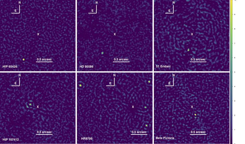
A&A proofs: manuscript no. paperF100IIfinalb

Article number, page 2 of 30
M. Langlois et al.: The SPHERE infrared survey for exoplanets (SHINE). II.

1. Introduction and context                                            differential image processing. With enhanced detection perfor-
                                                                       mances, the objective is to significantly increase the number of
The discovery of the first brown dwarf companion Gl 229 B ben-         imaged planets to characterize, but also to provide better statisti-
efited from the combined technological innovation of infrared          cal constraints on the occurrence and the characteristics of exo-
detectors and high contrast techniques (Nakajima et al. 1995).         planets at wide orbits (>10 au). This should give us a more global
Following this discovery, the first generation of dedicated planet     picture of planetary systems architecture at all orbits to improve
imagers on 10-m class telescopes (NaCo at VLT, NIRC2 at Keck,          our understanding of planetary formation and evolution mecha-
NICI at Gemini) conducted systematic surveys of young and              nisms. Early-results already confirm the gain in terms of detec-
nearby stars. They led the first direct detections of planetary        tion performances compared with the first generation of planet
mass companions in the early 2000’s. These companions were             imagers (Nielsen et al. 2019; Vigan et al. 2020).
detected at distances larger than several hundreds astronomical             The near-infrared wavelengths (H and K-bands) have been
units (au) and/or with a mass ratio not much smaller than a tenth      used intensively. They are a good compromise between low-
with respect to their host primaries (except for brown dwarf pri-      background noise, high angular resolution and good Strehl cor-
maries), giving hints of formation via gravo-turbulent fragmen-        rection. However, thermal imaging at L or M-bands has been
tation (Hennebelle & Chabrier 2011) or gravitational disk insta-       very competitive in terms of detection performances as the
bility (Boss 1997). Thanks to the improvement of direct imag-          planet-star contrast and the Strehl correction are more favorable
ing observation and data analysis techniques with ground-based         in those wavelengths despite an increased thermal background
adaptive optics systems (AO) or space telescopes, a few plan-          and larger inner working angle. For instance, SPHERE could be
etary mass objects and low-mass brown dwarfs have been de-             in some cases less sensitive than NaCo for the detection of giant
tected since the first detection by Chauvin et al. (2004). More-       planets around young, nearby M dwarfs at typical separations
over, these developments, enabled the discoveries of giant plan-       larger than 500-1000 mas.
ets within 100 au around young, nearby, and dusty early type                Both SHINE and GPIES surveys have recently discovered
stars like HR8799 b,c,d,e (Marois et al. 2008, 2010), β Pictoris b     three new exoplanets (Macintosh et al. 2015; Chauvin et al.
(Lagrange et al. 2009), and more recently HD 95086 b (Rameau           2017b; Keppler et al. 2018), and a few additional higher mass
et al. 2013a), and GJ 504 b (Kuzuhara et al. 2013a).                   brown dwarfs (Konopacky et al. 2016; Cheetham et al. 2018).
     Direct imaging is the only viable technique to probe for plan-    Smaller surveys using SPHERE and GPI also discovered several
ets at large separations with single epoch observations, but de-       substellar companions (Milli et al. 2017a; Wagner et al. 2020;
tecting them requires to overcome the difficulties caused by the       Bohn et al. 2020). They offer unprecedented detection, astromet-
angular proximity and the high contrast involved. With improved        ric and spectrophotometric capabilities which allow us to charac-
instruments and data reduction techniques, we are currently ini-       terize fainter and closer giant planets, such as the recent discov-
tiating the characterization of the giant planet population at wide    ery of 51 Eri b (2 MJup at 14 au, T5-type, of age 20 Myr; Mac-
orbits, between typically 10-100 au. More than a decade of direct      intosh et al. 2015; Samland et al. 2017), HIP 65426 b, a young,
imaging surveys targeting several hundred young, nearby stars          warm, and dusty L5-L7 massive jovian planet located at about
have lead to the discovery of approximately a dozen sub-stellar        92 au from its host star (Chauvin et al. 2017b), and the young
companions excluding the companions to brown dwarfs located            solar analogue PDS 70 now known to actually host two plan-
in the star vicinity (within 100 au). Despite the relatively small     ets PDS 70 b discovered during the SHINE campaign (Keppler
number of discoveries compared with other techniques, such as          et al. 2018; Müller et al. 2018) and PDS 70 c by MUSE (Haf-
radial velocity and transit, each new imaged giant planet has pro-     fert et al. 2018). Such surveys also provide key spectral and or-
vided unique clues on the formation, evolution and physics of          bital characterisation data for known exoplanets (e.g. De Rosa
young massive Jupiters.                                                et al. 2016; Samland et al. 2017; Chauvin et al. 2018; Wang
     Early surveys performed using the first generation of planet      et al. 2018; Cheetham et al. 2019; Lagrange et al. 2019; Maire
imagers enabled to conduct systematic surveys relatively mod-          et al. 2019). Despite these new discoveries, SHINE and GPIES
est in size sampling each less than hundreds of young nearby           have yielded significantly fewer exoplanet detections than pre-
stars (Chauvin et al. 2018). Various strategies were followed          dicted using extrapolations of radial velocity planet populations
for the target selection of these surveys: i/ complete census          to larger semi-major axes (e.g. Cumming et al. 2008). This re-
of given associations (Chauvin et al. 2003; Masciadri et al.           sults in setting strong statistical constraints on the distribution of
2005; Kasper et al. 2007; Chauvin et al. 2010), ii/ selection          giant exoplanets at separations >10 au from their stars, as well
of young, intermediate-mass stars (Janson et al. 2011; Rameau          as sub-stellar companions to young stars (Nielsen et al. 2019;
et al. 2013b; Nielsen et al. 2013), iii/ or very low-mass stars (De-   Vigan et al. 2020). As these systems are young (
A&A proofs: manuscript no. paperF100IIfinalb

we describe the reduction and calibration of the data sets. Sec-      used for the IRDIFS and IRDIFS-EXT observations respectively,
tion 4 is dedicated to the main results of the survey, including      and in IRDIS all first epoch observations were performed with
the detection limits of the survey. Finally, we summarize, in Sect    the DB-H23 and DB-K12 dual-band filter pairs (Vigan et al.
5, the characterization of newly discovered and known substellar      2010). Due to the presence of known companions and/or the de-
companions along with a description of the circumstellar disks        tection of (new) candidate companions, some targets were ob-
detected within the survey data. The conclusions and prospects        served multiple times for astrometric monitoring. In addition
are drawn in section 7. The relative astrometry and photometry        to the initial selected filters, follow-up observations were per-
of companion candidates from the sample is listed in Annex A.         formed in different configurations with IRDIS, for example with
                                                                      the broad-band BB-H and dual-band DB-J23 filters, as listed in
                                                                      the filter column of Table 1. This resulted in a varying number
2. The SHINE survey
                                                                      of observations for each target.
The SpHere INfrared survey for Exoplanets (SHINE: Chauvin
et al. 2017a) has been designed for 200 telescope nights, allo-
                                                                      2.2. Observations Optimized planning: SPOT
cated in visitor mode, using the SPHERE consortium guaran-
teed time. SHINE has been designed by the SPHERE consor-              Given the large number of targets, each associated with a prior-
tium to: (i) identify and characterized new planetary and brown       ity and an urgency (how soon the observation has to be made),
dwarf companions; (ii) study the architecture of planetary sys-       and the various observing constrains, including those connected
tems (multiplicity and dynamical interactions); (iii) investigate     to Angular Differential Imaging (ADI: Marois et al. 2006) obser-
the link between the presence of planets and disks (in synergy        vations, we built a dedicated tool, SPOT, to deliver an optimised
with the GTO program aimed at disk characterization); (iv) de-        scheduling of the observations, both on long and short terms.
termine the frequency of giant planets beyond 10 au; (v) investi-     SPOT is based on simulated annealing. It is described in in de-
gate the impact of stellar mass (and even age if possible) on the     tails in Lagrange et al. (2016).
frequency and characteristics of planetary companions over the             In brief, SPOT uses as inputs the calendar of allocated ob-
range 0.5 to 3.0 M .                                                  serving nights, the list of targets available for e.g. the whole
    The SHINE survey started in February 2015 and will be com-        semester, together with their associated instrumental set up (that
pleted in mid-2021, with observations of 500 targets out of a         is associated with specific overheads) and any specific schedul-
larger sample of 800 nearby young stars aiming at searching for       ing constrains (needed for second epoch observations), the tar-
new sub-stellar companions. The sample is oversized with re-          gets coordinates and magnitude, the minimal coronagraphic ex-
spect to the available telescope time by a factor of approximately    position duration, the maximum air mass, the maximum propor-
two, on the basis of the adopted observing strategy, which re-        tion (in time) of the observation that is allowed either before
lies on observations surrounding meridian passage in order to         or after the meridian crossing, the minimum exposure time, the
achieve the maximum field-of-view (FoV) rotation for optimal          amount of FoV rotation during the observation. It must be noted
angular differential imaging. This requires some flexibility in the   that the amount of FoV rotation depends on the target coordi-
target list in order to optimize the scheduling.                      nates and on the actual time and duration of observations. As it
    The general design of the survey, the sample selection and        also drives the exposure time, we also set a maximum exposition
the simulations performed for building it, the parameters of the      time, to avoid extending too much the duration of the exposure.
individual targets used in this early statistical analysis, and the        Classical, additional scheduling constraints are applied on
general properties of the sample used in this series of papers are    all targets: minimal angular distance to the Moon, avoidance of
described in detail in Desidera et al. (submitted). We describe       zenith observations. Poor atmospheric conditions may also be
in this paper early results obtained from the analysis of about a     taken into account through pointing restrictions that usually de-
third of the large SHINE survey sample, considering only those        pend on the wind direction and speed and through magnitude re-
targets whose first observations were done before Feb 2017.Sev-       strictions in case of non photometric conditions. Finally, SPOT
eral second epochs observations were also performed between           also takes into account the various overheads and the need for
2016 and 2019 to discriminate companions from background              astrometric and spectro-photometric calibrations. The astromet-
stars on the selected sample described in this paper. This selected   ric calibrations were to be observed as much as possible in the
sample dataset including 150 targets, is already large enough for     first night of each run, and the spectro-photometric in the fol-
reviewing the survey efficiency, to discuss the incidence of mas-     lowing night. After optimisation SPOT returns a schedule, and
sive planets at a separation > 10 au, and to have new indications     produces the Observing Blocks (OBs) that can be automatically
about the formation scenarios for giant planets.                      transferred to P2 (the ESO observing preparation tool).
                                                                           In practice, we generally request the coronagraphic data to be
2.1. Observations setup                                               obtained while the target is crossing the meridian at least 15 min
                                                                      before and after the meridian passage, and with at least 30 de-
All the observations were performed with the Spectro-                 grees of FoV rotation, unless it required more than 7200 s. The
Polarimeter High-contrast Exoplanet REsearch (SPHERE;                 minimum exposure time was set to 3600 s. The scheduling of
Beuzit et al. 2019) combining its SAXO extreme adaptive optics        the targets was always optimal; the efficiency of the night could
system (Fusco et al. 2006; Sauvage et al. 2016; Fusco et al. 2014)    be as high as 100% when typically 2-3 time more targets were
and its apodized pupil Lyot coronagraphs (Boccaletti et al. 2008;     available than actually those scheduled. Yet, when not enough
Carbillet et al. 2011; Guerri et al. 2011). Observations were ac-     targets were available as inputs, short (typically 30 min) holes
quired in either IRDIFS or IRDIFS-EXT mode, i.e. with both            could be present in the schedules during the nights. These holes
NIR sub-systems, IFS (Claudi et al. 2008) and IRDIS (Dohlen           were used to observe fillers requiring short exposure times (bi-
et al. 2008), observing in parallel (Zurlo et al. 2014; Mesa et al.   naries, stars with RV trends, astrometric and spectrophotometric
2015). The IFS covers a 1.700 ×1.700 FoV and IRDIS covers a           standards). By comparing with other surveys executed in service
more or less circular, unvignetted FoV of diameter ∼900 . The         such as BEAST (Janson et al., in preparation), we conclude that
APLC_YJHs and APLC_Ks coronagraphic configurations were               use of SPOT allowed an increase of more than 30% in the field
Article number, page 4 of 30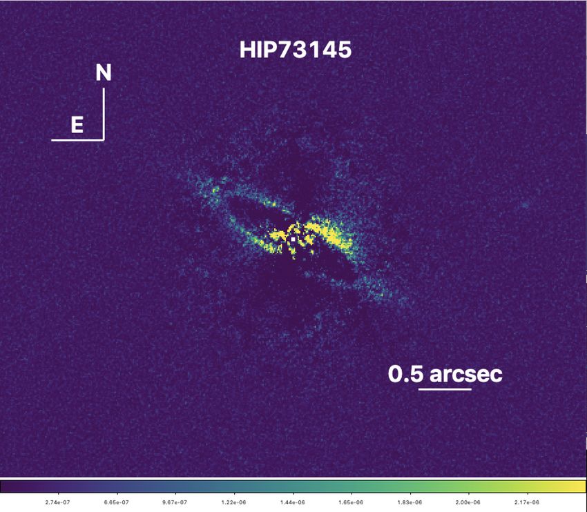
M. Langlois et al.: The SPHERE infrared survey for exoplanets (SHINE). II.

rotation angles for identical observing time with respect to the          large scatter in the Strehl distributions indicates that the seeing
service scheduling routinely used at ESO.                                 is also, as expected, a parameter influencing the Strehl among
                                                                          others such as τ0 and the star magnitude. Despite this large scat-
                                                                          ter the (Top Left) plot from the same Figure shows a linear de-
2.3. Observing conditions and Data quality
                                                                          crease trend of the Strehl with the seeing. This decrease is on av-
The SPHERE Instruments are fed by an extreme adaptive optics              erage 1.8% Strehl for an increase in seeing of 0.1” which is sim-
(AO) system called SAXO. It delivers a very high Strehl ratio,            ilar to the Strehl behavior versus seeing obtained by Milli et al.
which reaches above 90% in H-band for very good observing                 (2017b) when correction is applied according to the SPARTA
conditions by correcting both perturbations induced by the at-            versus DIMM measurements dependency. While the SPARTA
mospheric turbulence and from the internal aberrations of the             seeing provides an estimate which is closer to the image quality
instrument itself. A comprehensive description of the SAXO de-            in the science frames, it has been shown that the SPARTA see-
sign can be found in Fusco et al. (2016) and Beuzit et al. (2019).        ing estimations are smaller than the ESO DIMM measurements,
We derived here the overall statistical AO telemetry data from            a fact that may be accounted for the turbulence outer scale. The
SAXO and from the ESO MASS-DIMM measurements for the                      overall impact of the performance limitation from the seeing on
survey observations and relate these parameters to the Strehl ra-         our survey is clearly important as illustrated by the large number
tio, raw contrast and processed contrast in order to evaluate the         of observations occurring for seeing greater than 0.8” (Fig. 1 -
performance constraints from these observations. The telemetry            Top-Left).
data points are spread over 130 different nights and cover more                The Top-Right part of Fig. 1 shows the distribution of the
than 200 different observations. The AO telemetry data (avail-            Strehl as a function of the coherence time for our full sample.
able for a large number of our survey observations) includes es-          There is a steep rise in Strehl ratio with the coherence time (for
timates from the real-time computer (called SPARTA) several               τ0 < 3 ms) followed by plateau for larger coherence times (for
quantities of interest that could be related to the final perfor-         τ0 < 5 ms). This shows that for low coherence times, the AO per-
mances (hereafter SPARTA data) such as: the Strehl ratio and              formances are limited by the temporal bandwidth error as men-
additional atmospheric parameters including the seeing and the            tioned in Cantalloube et al. (2020) which also derives a 3 ms
coherence time. The Strehl is defined at 1.6 µm, while the seeing         threshold from the system point of view. This is in agreement
and coherence time are defined at 500 nm.                                 with the laboratory and first on-sky measurements described in
     These quantities are also connected here with the brightness         details in Petit et al. (2012). The overall impact of this perfor-
of the target (V and H magnitudes), retrieved from the Simbad             mance limitation on our survey is likely important as illustrated
database, and used as a proxy in V-Band for the number of pho-            by the large number of observations occurring when τ0 < 4 ms
tons received by the WFS1 . The distribution in magnitude for             (i.e 70% of the observations). Further analysis of the impact of
the sample considered here (for targets with telemetry measure-           this effect should include the seeing contribution in the Strehl
ments) is shown in Fig. 1 (Bottom Right). It illustrates the fact         error budget to disentangle the seeing and coherence time corre-
that our target selection as described in Desidera et al. (submit-        lations.
ted) was based on setting a magnitude limit (V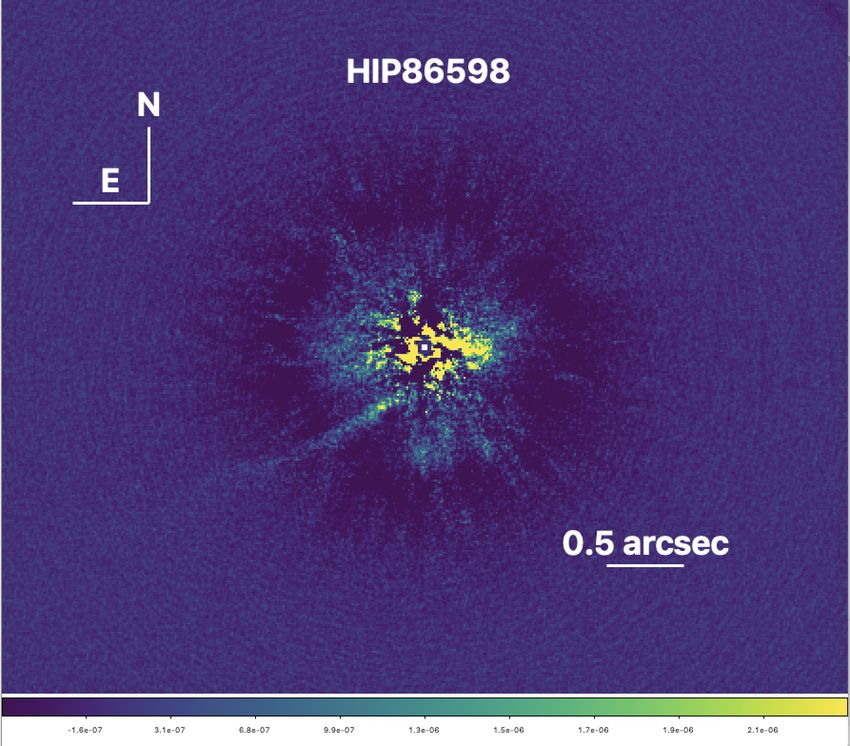
A&A proofs: manuscript no. paperF100IIfinalb

Fig. 1: Observing conditions and AO performances in IRDIFS observing mode: (Top-Left) Strehl ratio as a function of the seeing
measured by SPARTA. (Top-Right) Strehl Ratio as function of the atmospheric coherence time estimated by SPARTA. A linear fit
is overlaid in red on the Top figures. (Bottom-Left) Strehl ratio as function of the star V magnitude. The blue data points represent
the data taken with coherence time smaller than 3 ms.(Bottom-Right) Histogram illustrating the repartition of the observations
(including multiple observations of the same target) as function of the star magnitude in V (dark blue) and H-bands (light blue). The
apparent large number of observations of R=3.5 stars is an artificial effect due to the large number of observations targeting Beta
Pictoris.

3.1. SPHERE Calibration                                                rate (sub-mas) astrometry from Hubble Space Telescope (HST)
                                                                       or ground-based diffraction limited observations: 47 Tuc (Bellini
3.1.1. Astrometry                                                      et al. 2014; Soto et al. 2017; Bellini et al. 2017); NGC 6380
We present in this section the astrometric calibration of the          (Bellini et al. 2011; Soto et al. 2017) and Noyola (private com-
SHINE survey which depends on several factors described in             munication); NGC 3603 (Harayama et al. 2008; Khorrami et al.
detail in the following paragraphs: i/ platescale, True North and      2016; Rochau et al. 2010); and Trapezium B1-B4 (Close et al.
distorsion correction, ii/ angular offset (between field and pupil-    2012, 2013) (see Figure 2).
tracking and parallactic angle correction), iii/ star-centering.           IRDIS was used for all astrometric calibrations, because its
This section also presents as a conclusion, iv/ a sanity check of      field of view allows observation of a large number of stars, in
the calibration startegy based on Gaia-DR2 results.                    most cases between 50 and 100. Only seven stars were available
                                                                       for the Trapezium B1-B4 field, leading to a less accurate cali-
                                                                       bration of the field orientation (by 1%) and on the plate scale
Platescale, True North and distorsion An extensive descrip-            (by 0.1%), and was used only when the other calibration fields
tion of astrometry with SPHERE can be found in Maire et al.            were not accessible from February 2015 to March 2016. Due to
(2016b) and Beuzit et al. (2019). For what concerns in partic-         the less good accuracy of the catalog positions for NGC 6380
ular the SHINE survey, the astrometric calibration consisted in        and the smaller number of calibrating objects, we used this field
the correction for the instrument anamorphism (0.60±0.02% be-          only twice in May-June 2015 and once in June 2017. Using sev-
tween the horizontal and vertical directions of the detector, i.e. 6   eral calibrators enable to perform calibrations throughout the
mas at 1 arcsec), correction for constant offset angles (between       year and to do cross-calibration. Because the coronagraph has
the IFS and IRDIS fields of view, between pupil-tracking mode          a small effect on the pixel scale, the astrometric fields were ob-
and field-tracking mode), and determination of the values for the      served with a coronagraphic plate (including an offset for the
pixel scale and the correction to the true north. We find small but    Trapezium B1-B4 field observation, to shift the B1 star out of
non negligible variations of the last quantities with time requir-     the coronagraphic mask).
ing dedicated calibration for each observing runs. Appropriate             The pixel scale is slightly different for the H2, H3, K1, and
values were estimated for each run using several reference fields      K2 filters, with mean values of 12.255, 12.250, 12.267, and
of view in clusters with a large number of stars and having accu-      12.263 mas/pixel, respectively. For IFS, we used a constant value
Article number, page 6 of 30
M. Langlois et al.: The SPHERE infrared survey for exoplanets (SHINE). II.

Fig. 2: IRDIS H2 images of the fields used for the astrometric calibration. Upper left panel: 47 Tuc; upper right panel: NGC 3603;
lower left panel: NGC 6380; lower right panel: Orion B1B4. A logarithmic intensity scale is used to show also faint stars.

of the pixel scale of 7.46 ± 0.02 mas/pixel. Variations in this case   mode for ADI purposes, the astrometric fields were observed in
have less impact on the results due to the small field of view.        field-tracking mode. The offset between the pupil-tracking and
The typical measurement accuracy of the pixel scale is ±0.012          field-tracking modes was measured at the beginning of the sur-
mas/pixel using our two best fields 47 Tuc and NGC 3603, while         vey to be equal to -135.99±0.11 degree. The parallactic angle
the true north correction (weighted value -1.77 degree) typically      is computed from the data FITS header: timestamp, RA/DEC of
has an error of ±0.07 degree. For IFS, an additional offset of         the derotator (INS4.DROT2.RA/DEC) which are more accurate
100.48 degree in the clockwise direction is applied to account for     than the "RA" and "DEC" keywords (J2000 coordinates of the
the orientation of the instrument FOV. This leads to uncertainties     target). In case these parameters are used it is possible to cor-
in the position of 3–4 mas at the edge of the IRDIS field of view      rect for the precession of coordinates between 2000 and the date
and less than 1 mas for IFS. For comparison, typical accuracy          of observation. In order to derive the precise parallactic angle
of GPI using their best calibrations are ±0.021 mas/pixel in the       of each DIT from the timestamp we also included a paramet-
pixel scale and ±0.12 degree in the true north correction (De          ric model of the overheads. We observe a systematic error in
Rosa et al. 2019). The better calibration accuracy obtained for        the parallactic angle estimation due to backlash in the derotator
SPHERE is due to the wider field of view of IRDIS that allows          mechanism of ∼0.05◦ , as demonstrated in Beuzit et al. (2019).
the use of stellar cluster fields as calibrators with more accurate    In pupil-stabilized mode, this leads to a ∼0.4 pixel difference in
catalog positions.                                                     the position of an object located at the edge of the IRDIS FoV
                                                                       on either side of the meridian.

Field/Pupil tracking and parallactic angle calibration While
the SHINE science observations are taken in pupil-tracking
                                                                                                              Article number, page 7 of 30
A&A proofs: manuscript no. paperF100IIfinalb

Star centering The astrometry we consider in this paper is rel-            IRDIS FOV (sep>6.5 arcsec), both leading to inaccurate astrom-
ative to the star. Since the star point spread function peak is            etry. Gaia measurements are most likely unreliable for very high
hidden by the coronagraphic mask and to avoid concerns due                 contrasts. This is the case of HD1160C, for which the Gaia con-
to the non uniform intensity distribution of the coronagraphic             trast is 8.24 mag. Binary periods for these stars are so long that
leakage, its position was determined using a special calibration           they should not affect the result. However, a couple of the ob-
(STAR-CENTER) where four faint replicas of the star image are              jects are not binaries but rather background stars (HIP82430 and
created by giving a bi-dimensional sinusoidal profile to the de-           PDS 70). We took into account the relative proper motion be-
formable mirror (see Beuzit et al. 2019; Makidon et al. 2005).             tween the SHINE observation and the Gaia epoch (2015.5). At
The STAR-CENTER calibration was repeated before and after                  the end we have seven good comparative measurements.The sep-
each science observation, and results center estimations were av-          aration measured by SHINE is slightly larger than that measured
eraged. While this calibration greatly reduces uncertainties in the        by Gaia DR2. The mean offset is −2.8 ± 1.5 mas, with a root
exact position of the star and the center of the field rotation, ex-       mean square (rms) of 3.9 mas. The position angle measured by
perience shows that small drifts of a few mas of the star center           SHINE is similar to that measured by Gaia DR2: the mean off-
during long sequences of ∼1–2h can occur. For this reason in or-           set is 0.06 ± 0.04 degree, with an rms= 0.11 degree. The rms
der to increase the star centering accuracy, we generally used, for        agrees well with the expected uncertainties in these quantities in
the second epochs, when doing (candidate) companions follow                the SPHERE data.
up, the STAR-CENTER setup solely for the science exposure.                     We conclude that the minimum accuracy of the astrometric
    We performed specific measurements to estimate the accu-               calibration of SHINE data is ±2 mas at separations < 1 arcsec,
racy of the central star position when the STAR-CENTER setup               and ±3 mas at larger separations. These values are similar to
is not used for the science exposure (i.e most cases presented             the scatter typically observed for GPI astrometric calibrators (De
in this paper). To do so we measured the position of the central           Rosa et al. 2019). In practice, the astrometric accuracy on the
diffraction peak on the IFS datacubes collapsed in wavelengths,            position of faint substellar companions detected in the SHINE
and making the mean over all Detector Integration Time (DIT);              data is limited by the measurement uncertainties from the image
as mentioned above, errors are likely independent of the errors            post-processing (Sect. 3.3) and by the companion magnitude.
in the STAR-CENTER procedure. We found that the mean posi-
tion of the center is offset with respect to the nominal position
along the Left-Right direction in the pupil reference frame by a           3.1.2. Photometry
small but significant amount 0.52 ± 0.10 mas for Y-H observa-              We describe below the strategy to derive the relative photom-
tions, while there is no offset for the Y-J mode (0.03 ± 0.05 mas)         etry of the SHINE candidates considering the unsaturated and
or along the Top-Bottom direction in the pupil reference frame in          coronographic observations of a scientific target, and two tests
both modes. The root mean square (rms) scatter of the residuals            done by using IFS to validate our strategy for both IRDIS and
after a 3-σ clipping are 1.35 mas (1.23 mas) in RA and 1.24 mas            IFS which have very similar photometric biases.
(1.43 mas) in declination, for the Y-H (Y-J) mode. Most outliers
are found in data sets that were not validated and a few of them
are binaries. There are 5% of the validated observations that have         Strategy In the SHINE survey, photometry of candidate com-
much larger dispersion of the position of the peak than usual;             panions and limiting magnitudes for non detections are relative
these anomalous cases make ∼10% of the observations acquired               in contrast to the central star. Since the star is behind the coro-
before February 2016, while the fraction reduces to ∼2% after              nagraphic mask, simultaneous photometry is not possible. We
that epoch. This is likely due to improvements in the AO cali-             thus include a flux calibration (STAR-FLUX) for both IRDIS and
bration, that resulted in less distorted diffraction peaks. A few          IFS that is acquired just before and after the science exposure
of these residual cases may be unresolved binaries. We conclude            by offsetting the Differential Tip-Tilt Stage (DTTS) by about 0.5
that a reasonable estimate for the accuracy of the absolute central        arcsec with respect the coronagraphic mask using the SPHERE
star position is ±1.5 mas for both IFS and IRDIS.                          tip/tilt mirror (Beuzit et al. 2019). When performing this calibra-
                                                                           tion, suitable neutral density filters are inserted to avoid detector
                                                                           saturation. The transmissions of these neutral density filters were
Cross-check with Gaia DR2 An external check of the accu-                   carefully calibrated from 0.9 to 2.3 microns (see Beuzit et al.
racy of our astrometry is provided by wide companions in the               2019 and ESO website 3 ) and are taken into account for the con-
Gaia Data Release 2 catalogue (Gaia Collaboration et al. 2018).            trast estimation. This procedure works very well in stable condi-
The number of sources in the IRDIS field of view with a con-               tions, but it may be affected by variations of the Strehl ratio from
trast adequate to be detected with Gaia is limited because stars           evolving observing conditions. Higher photometric accuracy can
with known bright companions were not included in our sam-                 be achieved by using the waffle pattern continuously (for com-
ple to avoid problems for the AO and heavy saturation of the               panion candidates follow up) during the observing sequence to
detector. By comparison with the SPHERE results, we find that              monitor the Strehl variations.
Gaia DR2 limiting contrast (in the visual G-band) corresponds
to contrasts in the near infrared of ∆H=2.5 mag for separation
sep< 2.5 arcsec and 6 mag for sep> 4 arcsec2 . For this com-               Cross-check with catalogues and binary companions A first
parison, we considered 34 IRDIS close companion candidates                 test of the photometric calibration accuracy is provided by com-
(some of them not included in the sample described in this pa-             paring the peak counts of the diffraction image of the flux cal-
per) with ∆H2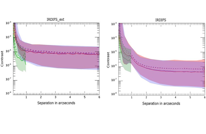
M. Langlois et al.: The SPHERE infrared survey for exoplanets (SHINE). II.

Fig. 3: Spectra of the white dwarfs used as spectrophotometric standards compared with predictions from model atmospheres (solid
lines). Different symbols are results obtained from different epochs. We normalized the observed spectra at the median flux in a
narrow range around 1.25 micron.

ity and the impact of variability on the Strehl ratio. Using J-band     of the spectra determined by our method with atmospheric mod-
IFS data, we obtain an rms of residuals of 0.15 mag for observa-        els is given in Figure 3.
tion in the Y-H mode, and 0.19 mag for those in the Y-J mode.                We conclude from these measurements that a reasonable
This has been computed after eliminating the expected variations        photometric errors estimate for both the limiting contrast and
due the Strehl ratio and after clipping outliers deviating greater      for companions characterisation (not including the ADI post
than 2.5 standard deviation from the mean with an iterative pro-        processing error contribution), is around ±0.2 mag. It is domi-
cedure (about 12% of the data). A similar value is obtained by          nated by the STAR-FLUX variation which is also the case for
considering the rms scatter of the estimate of the coronagraph          the survey data photometric error which is on average equal to
central transmission - measured as the ratio between the maxi-          ±0.25 mag.
mum counts of the diffraction peak in the coronagraphic image
and in the flux calibration (corrected for the length of the integra-
tion and neutral density filter transmission). The average corona-      3.2. SPHERE Data Center preprocessing
graphic transmission measured in this way are 0.00168±0.00005           3.2.1. IRDIS-only steps
for the Y-H mode, and 0.00208 ± 0.00001 for the Y-J mode, re-
spectively, for a median SHINE observation.                             The SHINE survey was reduced by the SPHERE Data Cen-
                                                                        tre (hereafter SPHERE-DC) 4 . For IRDIS data, the first reduc-
                                                                        tions steps (dark/background, flat, and bad pixel correction) rely
    A second test of the photometric calibration accuracy is pro-       on the SPHERE Data Reduction and Handling (hereafter DRH)
vided by the photometry of three standard systems (HD2133,              pipeline Pavlov et al. (2008) provided by ESO. We used the on
HD114174, and REJ1925-563) composed of a main sequence                  sky background because there is a significant difference between
star and a white dwarf with separations in the range 0.2-0.7 arc-       day-time background calibrations and the on sky background
sec, we have observed during the survey. These systems were ob-         recorded in the science frames. This is the case mostly in K-
served several times, with typically at least one observation per       band with a systematic, spatially variable, offset (typically of the
run. For schedule optimization, these observations were acquired        order of 100 ADU for 64s exposure time) which is due to the sky
in ADI with the star quite far from meridian and in poorer ob-          background contribution itself. A similar effect is also visible in
serving conditions, than typical survey targets: we consider here       H-band, on a smaller level (typically of only few ADU).
only those observations that were obtained in fair to good atmo-            Since most of the SHINE observations use the pupil-tracking
spheric conditions. Photometry of the faint companions was ob-          observing mode, a very accurate determination of the star center
tained by inserting a negative scaled point spread function at the      is needed in order to successfully use both the angular differ-
position of the companion in the raw datacube, i.e before com-          ential imaging and spectral differential imaging methods. Also
bining the various DITs. We then measured the rms residuals             since IRDIS is used in dual-band imaging, the star center in both
of the differential image obtained through monochromatic prin-          IRDIS channels is used to combine them. By default, we use
cipal component analysis (PCA: Soummer et al. 2012) around              the DRH sph-ird-star-center routine to determine the star
the companion. The procedure then minimizes these residuals             center position, using the waffle images acquired for this pur-
by simultaneously adjusting the contrast and the position. The          pose just before and after the science observations. This very
values we consider are the mean of the results obtained using           fast routine provides an accurate centering in many cases, but
2 to 6 PCA modes. The average contrasts in the J-band ob-               could fail for weak waffle spots, especially in the K-band where
tained with this procedure using the main sequence star and             these spots can be hidden beneath a much stronger thermal back-
the white dwarfs are 7.68, 10.04, and 6.10 mag for HD2133,              ground noise but also when the deformable mirror offsets to cre-
HD114174, and REJ1925-563, respectively. The rms value for              ate this pattern are set too low. We therefore designed an auto-
the contrasts in the J-band/H-band are 0.11/0.05, 0.18/0.08, and        mated way to check the quality of the DRH centering by com-
0.05/0.07 mag for HD2133 (8 observations), HD114174 (14 ob-             paring the two center positions derived out of the four waffles.
servations) and REJ1925-563 (6 observations). The photometric           When the distance between these two possible center positions
errors as expected increase with magnitude and as a consequence         was found to be greater than 0.9 pixel, we used a SPHERE-DC
are smaller in H-band than in J-band. This may be also attributed       made IDL routine that is more robust to identify weak waffle
to a higher impact of the variation of the SR and of the speckle
                                                                        4
noise for fainter targets and shorter wavelengths. A comparison             http://sphere.osug.fr/spip.php?rubrique16&lang=en

                                                                                                                Article number, page 9 of 30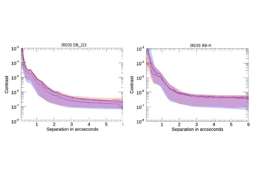
A&A proofs: manuscript no. paperF100IIfinalb

spots. This routine is able to detect weaker waffles by locat-           et al. (2018) software which offers various ADI options. We
ing them within small circular apertures located at the expected         selected for the homogeneous reduction TLOCI (Marois et al.
(wavelength-dependent) position and by using in combination a            2014; Galicher et al. 2018) and Principal Component Analysis
high-pass spatial filtering, sky-background subtraction and me-          (PCA: Soummer et al. 2012) for IRDIS and PCA Angular and
dian stacks of all waffle images available in order to increase          Spectral Differential Imaging (ASDI: Mesa et al. 2015) for IFS.
their SNR.                                                                    In the TLOCI approach (Lafrenière et al. 2007), the PSF-
    A small fraction of the SHINE datasets use continuous waffle         reference is estimated for each frame and each location. Linear
mode observations, meaning that the waffle spots are activated           combinations of all data are computed to minimize the residuals
during the entire observation, for better astrometric monitoring         into an optimization zone, which is much bigger than the sub-
(with some localized loss in the limiting contrast because of the        traction zone to avoid the self-removal of point-like sources.The
secondary spots). In this specific cases, we perform individual          SpeCal version of the TLOCI algorithm is derived from the one
re-centering of each frame in the sequence using the SPHERE-             described in Galicher et al. (2018) assuming a flat planet spec-
DC dedicated star-centering routine described above. This im-            trum in contrast. Adjustable parameters are used to select the
proves the quality by correcting any drift or jitter of the targeted     frames and to describe the regions of interest. In SpeCal, the
star behind the coronagraph, and as a result improves the quality        gap between this region and the region of interest is set to 0.5
of the astrometric measurements by removing these sources of             Full Width Half-Maximum (FWHM). Hence, the optimizing re-
error.                                                                   gion is far enough from the region of interest so that the flux of a
                                                                         source in the latter does not significantly bias the linear combina-
                                                                         tion. Finally, an additional parameter sets the radial width of the
3.2.2. IFS-steps                                                         optimizing region. We considered here a radial width of the sub-
For IFS data we use the Data Reduction and Handling (DRH                 traction zone of 1 FWHM in radius; a radial-to-azimuthal width
Pavlov et al. 2008) pipeline but complement it with additional           ratio of 1.5; a standard surface of the optimization zone was N =
steps implemented at the SPHERE Data Center (Mesa et al.                 20 PSF FWHM and 10% is used for the minimum residual flux
2015; Delorme et al. 2017a) to improve the wavelength cali-              ratio due to self subtraction compared to the flux of a putative
bration, apply a correction for cross-talk, and improve the han-         candidate.
dling of bad pixels. The improvements of the wavelength cali-                 For historical reasons, two PCA algorithms are implemented
bration are obtained by using a cubic fit whose coefficients are         in SpeCal. The first version can be applied on IRDIS or IFS
estimated from the wavelength shifts of the spots generated by           data using ADI or ASDI. This algorithm follows the equation
the STAR-CENTER calibration - that are known to scale linearly           of Soummer et al. (2012). In the ADI case, which is the option
with wavelength. The cross-talk correction is performed using            selected to reduce IRDIS data in this paper, the principal com-
an iterative procedure that corrects for the spectrograph PSF, us-       ponents are calculated for each spectral channel independently.
ing coefficients derived using appropriate tests performed in the        Each frame is then projected onto a limited number of modes. In
laboratory during the instrument assembly. Bad-pixels are cor-           the ASDI case, the algorithm is the same but it works simulta-
rected using a dedicated sky observation acquired at the end of          neously on the spatial and spectral frames. The second version
each science exposure. This procedure yields more accurate re-           of PCA used to reduce IFS data in this paper, is very similar to
sults than the one based on the flat field calibration within the        the first version we have described but it was applied only on
DRH.                                                                     IFS data using the ASDI option (Mesa et al. 2015). In addition,
                                                                         it is worth mentioning that both PCA algorithms we use have
                                                                         no frame selection to minimize the self-subtraction of point-like
3.2.3. Final steps common to IRDIS and IFS                               sources when deriving the principal components.
                                                                              For PCA and TLOCI algorithms that bias the photometry of
After these pre-reduction steps, both IRDIS and IFS datasets are         off -axis point sources, SpeCal estimates the throughput at each
corrected for the instrument anamorphism and the astrometric             position in the field by generating a datacube of fake planets for
solution (pixel scale and True north) estimated from the calibra-        which the ratio of the flux in the resulting image to the flux of the
tion described in Sec. 3.1.1 is applied to the dataset. The out-         fake planet is calculated to obtain the centro-symmetrical 1D-
put data is composed of a pre-reduced master cube combining              throughput as a function of the angular separation which is then
all frames obtained during a given observation sequence, that is         applied to the images. For PCA, Specal estimates the through-
used as input for all Angular Differential Imaging (ADI Marois           put by inserting fake planets injections which are only 10 times
et al. 2006) algorithms. We also associate to this master cube           brighter than the local stellar residuals level after PCA. This
a vector of de-rotation angles for each frames, using the accu-          makes it possible to be close to the level of interest while be-
rate timing and overheads for each frame, to produce a frame-to-         ing sufficiently above the residual to minimize the bias in the
frame determination of the parallactic angle.                            throughput estimation. For TLOCI, the throughput is calculated
                                                                         from an analytical formula (see section 2.10.2 of Galicher et al.
3.3. ADI and ASDI postprocessing                                         (2018). The contrast curves, we derived in the following, for
                                                                         each spectral channel are based on the azimuthal standard de-
For both IRDIS and IFS, we obtain a good-quality re-centered             viation calculated in annuli of 0.5 FWHM width. Finally, the
images gathered in a single master cube associated with their            5σ detection limits are derived by taking into account the flux
parallactic angle values. Subsequent steps follow to estimate and        loss from ADI self-subtractions, the transmission of the coro-
subtract the stellar halo from each images, followed by derota-          nagraph at short separations (close to the inner working angle
tion and stacking of the residuals. The most critical step is the es-    (IWA: 0.1”) and the transmission of the neutral-density filter if
timation of the stellar halo that drives the level of the noise resid-   used when registering the PSF. These detection limits are thus
uals. We applied different Angular Differential Imaging (ADI)            normalized by the unsaturated PSF flux. Both 1D and 2D con-
algorithms to optimize the detection performances and to iden-           trast maps are estimated following these steps for each star for
tify associated biases. We rely mainly on the SpeCal (Galicher           each reduction technique.
Article number, page 10 of 30
M. Langlois et al.: The SPHERE infrared survey for exoplanets (SHINE). II.
All target stars were processed for each instrument in a ho- 4. High contrast Performances
mogeneous way using at least TLOCI or PCA with similar sets
of parameters. We considered 50, 100 and 150 PCA modes for 4.1. Contrast curves
IFS and 5 for IRDIS. We inspected by eye at least three residual
maps for each star and for both IFS and IRDIS to look for candi- We derived the 5-σ IRDIS and IFS contrast curves of each ob-
date companions (CC). We also included small number statistic servation for all the targets in the sample as presented on Figures
correction. In addition to the standard SpeCal reductions, we also 4 and 5. These detection limits are derived based on the noise
used, on several cases, ANDROMEDA (Cantalloube et al. 2015) in the speckle-subtracted image, compensated for the through-
and PACO (Flasseur et al. 2018, 2020b) algorithms to search for put of the algorithm (calibrated with fake planet injections), the
points sources. Given their statistical robustness to derive detec- transmission of the coronagraph (calibrated from measurements
tion limits and to better identify false detections these algorithms in SPHERE), and the small sample statistics (Mawet et al. 2014).
will become the main algorithms for the final analysis of the More details are provided in Galicher et al. (2018). Two types of
SHINE survey. contrast are discussed in detail in this section: the raw contrast,
computed on the median coronagraphic image of each observa-
tion and the contrast after post-processing described above. As
3.4. Astrometric and Photometric extraction for point sources illustrated on Fig B.1 and B.4, the raw coronagraphic contrast at
various separations shows a strong dependency with the Strehl
PCA and TLOCI algorithms are known to distort the images of and seeing both estimated by the average of the SPARTA values
any off-axis point-like source. To retrieve accurately the relative during the coronagraphic sequence. The two smaller separations
photometry and astrometry of the detected candidate compan- (from 100 to 700 mas) are within the AO control radius located
ions (CC) with their uncertainties, SpeCal fits a model of an off- at 840 mas separation radius in the H-band.
axis point source image to the detected point source and adjusts
its position and flux to locally minimize the flux. After build- This dependency remains clearly visible on post-processed
ing a model of the point source using the technique described in data especially at 500 mas, despite other factors also coming into
(Galicher & Marois 2011), the flux and the position of this syn- considerations such as the field rotation and the stability of the
thetic image are adjusted within a disk of diameter 3 FWHM so conditions (see Fig B.2). At small separation, these scatter plots
that it includes the positive and the negative parts of the point shows that one can easily gain one magnitude in raw contrast
source image. To optimize the computation time, instead of cal- by increasing the Strehl by 10% or the decreasing the seeing by
culating the synthetic image each time we test a new planet po- 30%. As a consequence it is clear that conducting the survey in
sition, we shift the synthetic planet image to its rough position. visitor mode which does not offer the best seeing condition had
Once the optimization is completed, we measure the excursion some impact on the survey ultimate contrast performances. Out-
of each parameters that increases the minimum residual level by side the AO correction radius, at separation greater than 900 mas,
a factor of 1.15. These excursions correspond to the 1 σ accuracy there is still a smaller dependency of the contrast with the seeing
due to the fitting errors in the SpeCal outputs. The spectrum ex- due to the residual light scattering outside the AO control ra-
traction from IFS data is performed similarly by processing the dius and the lower height of the diffraction peak. As part of this
wavelength channels separately. For the channels with no detec- study, the dependency of the post-ADI contrast on parameters
tion above 1 σ we provide an estimation of the upper limit only. tracing the quality and stability of the conditions were also in-
In conclusion, we summarize the astrometric and photomet- vestigated as illustrated on Fig B.1, B.4 and B.2. We considered
ric error budget given by Specal considering both calibrations the dispersion in the seeing, coherence time, Strehl, during the
and ADI/ASDI extraction errors. duration of the pupil-stabilised sequence. No significant correla-
For astometry, this budget includes: tion could be drawn from this sample. It is worth noticing that at
small separation (100 mas) the processed contrast is lower than
1. calibration with uncertainties of the detector distorsion, plate the raw contrast because of the very small angular rotation, the
scale and True North, small throughput of the algorithm (from self subtraction) and the
2. determination of the correction for constant offset angles stronger coronagraphic residuals.
(between the IFS and IRDIS fields of view, between pupil- The gain from raw contrast to post-processed contrast is
tracking and field-tracking modes); clearly visible on Fig 6 which shows a typical improvement
3. calculation of the parallactic angle variation (correction of greater than 5 magnitudes at short separations for both IRDIS
precession and timestamp), and IFS. It is worth noticing that the contrast gain in the IFS
4. central star position, field of view is consistent for all separations and reach at least 7
5. determination of the companion/candidate relative position magnitude. For the shorter separation located at the edge of the
with Specal (Galicher et al. 2018). coronagraph (100 mas) there is marginal improvement for IFS
from ASDI and no improvement for IRDIS in contrast due to
For photometry, it includes:
the very small angular rotation, the small throughput of the algo-
1. Contrast estimation with proper calibration of neutral den- rithm and the stronger coronagraphic residuals for both instru-
sity, exposure time, and associated error related to the vari- ments. At larger separation than the AO cutoff, the improvement
ation between Start/End STAR-FLUX calibrations but not from the post-processing range from 2 to 4 magnitudes.
including the strehl variation during the observing sequence We also plot on Fig B.3 the processed contrast as function
(psf), of the star magnitude for both IFS and IRDIS at various separa-
2. Temporal variations of the stellar coronographic flux be- tions. From these figures it is clear that there seem to be small
tween 30-50 pixels during the observing sequence (Seq), correlation between these parameters when the post-processing
3. Companion flux determination considering ASDI signature, if performed using TLOCI. On the contrary the PCA method for
taking into account flux cancellation from the algorithm both IRDIS and IFS seems to be affected by the magnitude of
used, and coronograph attenuation correction as described the star at least for the largest separations which is likely related
in (Galicher et al. 2018). . to the noise from the instruments background.
Article number, page 11 of 30A&A proofs: manuscript no. paperF100IIfinalb
Fig. 4: Contrast curves at 5 σ obtained for the full sample for irdifs-ext (Left) and irdifs (right) modes observations. The solid line
gives the median value of the contrast. The dash line gives the mean value of the contrast. Red color is for IRDIS data reduced in
PCA ADI, Blue color is for IRDIS data reduced in TLOCI ADI, and green color is for IFS with PCA ASDI reduction
We also highlight that one clear cause of contrast degradation Vigan et al. (2020). For IRDIS contrast curves, we convert the
in the post-ADI contrast is the presence of a smooth halo within contrast curves using the evolutionary models computed in the
the AO-corrected region which results from either bad seeing or appropriate dual-band filter, while for the IFS contrast curves we
from high-altitude wind related to the jet stream as discussed in use the predictions in the J-band filter for YJ data and in the H-
(Cantalloube et al. 2018) leading to a non symmetrical halo in band filter for YJH data. As demonstrated in Vigan et al. (2015),
the direction of the wind (called the wind driven halo, WDH). this approach for the IFS detection limits provides an accurate
This halo is rotating in the pupil-stabilised data set because it is estimation of the detection limit.
fixed on the sky as described in (Cantalloube et al. 2020). In post- For a selection of companions presented in 5.1, we show
ADI frames, it therefore appears as a brighter elongation along the detection of planet-like limits achieved by the survey in Fig.
the wind direction, with negative counterparts at 90 degrees. The 10. Several targets appear to be relatively easy (HR 8799 bcd,
impact of this effect does not appear to be very strong on the HIP 65426 and HIP 64892) for this survey, allowing for exquisite
azimuthal averaged contrasts we have plotted but is noticeable characterisation. Other targets appear to be much more challeng-
on the 2D contrast maps. Increasing the temporal bandwidth of ing mainly because they are at separations closer than 20 AU.
SAXO is the foreseen solution to help mitigate this effect. This The detection limits for these typical objects reach few Jupiter
is considered as one option in a forthcoming upgrade of the in- masses at such small separation while it can reach around 1
strument, SPHERE+ (Boccaletti et al. 2020). Jupiter mass at separations greater than 50 AU.
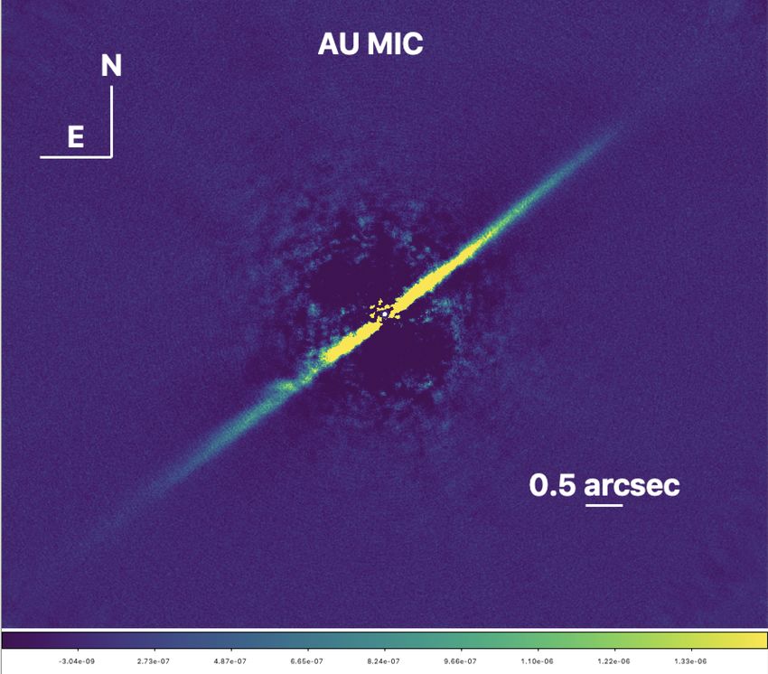
4.2. Mass detection limits 5. Exoplanet, Candidate Companion Detections
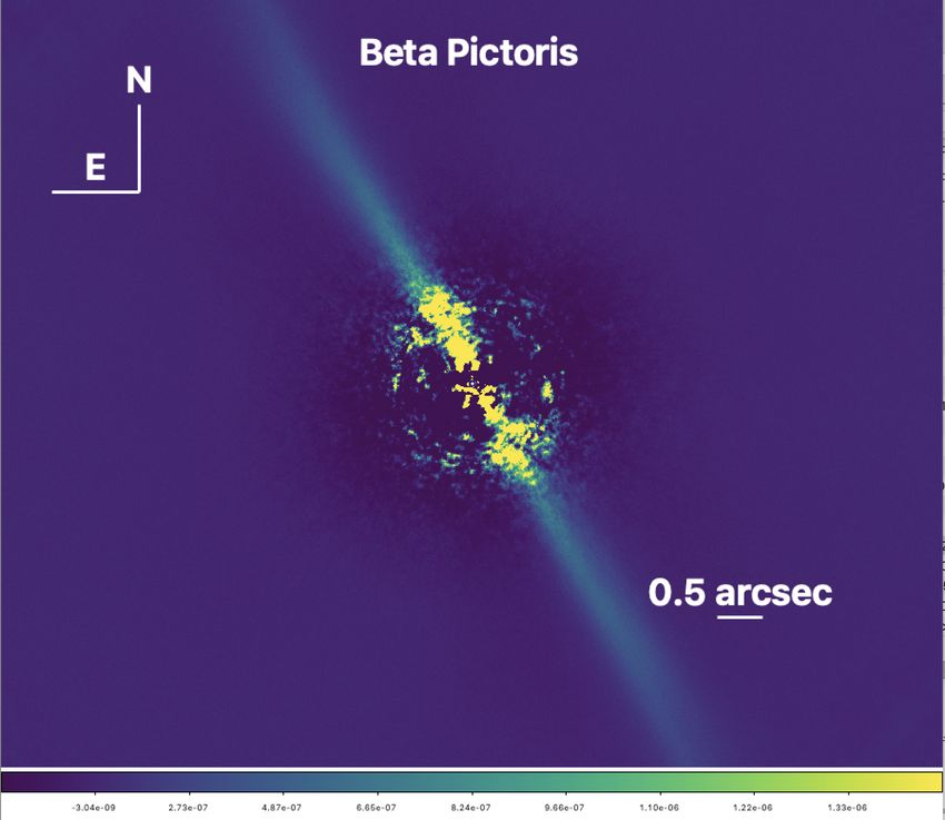
5.1. Brown dwarfs and exoplanets
The contrast curves are converted into mass limits using mass-
luminosity relationships. Whereas for old (& 1 Gyr) systems this A total of sixteen substellar companions were imaged in
relationship is essentially unique for gas giants at large sepa- the course of this part of the SHINE survey, including
ration (Burrows et al. 1997; Baraffe et al. 2003), at young ages seven brown dwarf companions (PZ Tel B, η Tel B, CD -
the value of the post-formation luminosity still remains uncertain 35 2722 B, HIP 78530 B, HIP 107412 B, GSC 8047-0232 B and
(Marley et al. 2007; Spiegel & Burrows 2012; Marleau & Cum- HIP 64892 B), and ten planetary-mass companions (51 Eri b, β
ming 2014). We present here a mass conversion of the contrast Pictoris b, HD 95086 b, HR8799 bcde, GJ 504 b, AB Pic b and
curves for a few specific targets using the canonical predictions HIP 65426 b). Two new companions have been discovered in
of the COND-2003 evolutionary models (Baraffe et al. 2003). this sample: the exoplanet HIP 65426 b (Chauvin et al. 2017b)
The impact of using other mass-luminosity relationships on the and the brown dwarf companion to HIP 64892 B (Cheetham
sensitivity of the SHINE survey are explored in more details in et al. 2018). PDS 70 was not originally part of the SHINE sam-
Article number, page 12 of 30You can also read