Extremely low frequency radio spectroscopy of the interstellar medium as important instrument of studies of the tenuous, cold, and partially ...

Extremely low frequency radio spectroscopy of the

interstellar medium as important instrument of studies of
    the tenuous, cold, and partially ionized objects.

            S.V. Stepkin, A.A. Konovalenko, D.V. Mukha.
      Institute of Radio Astronomy of the National Academy of
                          sciences of Ukraine
           4 Chevonopraporna St, Kharkov 61002, Ukraine.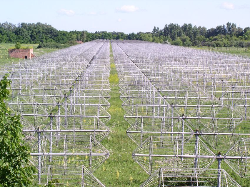

Abstract

Radio spectroscopy at extremely low frequencies provides unique opportunities
   for studies of the cold low-density partially ionized interstellar medium. The
     radio recombination lines (RRL) of carbon are observed in many galactic
   directions up to the middle decametric waves. The biggest atoms which have
    been detected in space with RRL correspond to quantum numbers as big as
     1009. Such atoms have a classical diameter of about 108 µ (~0.1 mm) and
   they are larger by a factor of ~ 106 compared to the ground state atom. The
  partially ionized and cold interstellar plasma can play significant role in many
     astrophysical phenomena (among them, for example, are processes of star
         formation). The experience obtained with the biggest low frequency
    instruments such as UTR-2 (Ukraine) shows that the low frequency carbon
        RRL can be observed not only against strong background source like
  Cassiopeia A but also against non thermal background galactic radio emission.
   It is confirmed by the detection of absorption carbon RRL in the direction of
  galactic plane at frequencies near 25 - 26 MHz. Low intensity of such features
       causes the necessity of really big instruments in order to carry out these
     investigations and LOFAR can open new spectrum of opportunities in the
                                         field.

Theory of RRL
RRLs are produced by transitions of recombining electrons between two
  atom levels in ionized gas. Their frequencies can be calculated using
  Rydberg’s formula:

             2  me 1        1
 ν n = cZ R(1 −    )( 2 −        2)
                M a n ( n + ∆ n)
c is speed of light, Z is the nuclear charge of the ion , R is the Rydberg
    constant for the taken species, me and Ma are electron and nuclear mass,
    n and ∆n are principal quantum number and its change.
The possibility of RRL observation was predicted by Kardashev in 1959.
    They were detected in 1963-1964 by Dravskikh and Dravskikh at 5.7 GHz
    (n=105) and Sorochenko and Borodzich at 8.9 GHz (n=91). A lot of high
    frequency RRL have been observed towards classical hot HII regions.
    Also, for example, they have been detected in planetary nebulae, external
    galaxies, and in some circumstellar envelopes.

n>600, ν< 30 MHz
∆TL/TC =-τL*bnβn=f(Ne, Te, S, ME)
τL*=2*106 Ne2 S/Te2. 5
The profile of RRL is determined by several broadening effects.
Doppler broadening caused both by thermal particles motion and
turbulence in the ISM leads to a Gaussian shape.
Collisions in the gas (Stark effect) and influence of background
radiation are responsible for a Lorentzian curve.

∆νD=∆νL ∆V/c
∆νp~Ne n5. 2
∆νR~n5. 8
The distance between adjacent features         δνL~3ν/n
In 20 … 30 MHz band there are ~ 90 lines.

RRL profile
The combination of Doppler and Lorentzian broadening
  effect produces a Voigt profile which is the convolution
  of the Gaussian and Lorentzian curves

                             ∞                 2
                  2 ln 2 a                e − t dt
         V (ν ) =
                   π ∆νDπ    ∫                                      2
                                      2 ln 2 (ν − ν 0 )        
                          .− ∞ a +
                                2                      −   t 
                                          ∆νD                  
where

                         ln 2∆ ν L
                  a=
                          ∆ν D

Observations of the very low frequency RRLs

Detection of carbon RRLs at 26 MHz in 1980 opened new
  field of extremely low frequency radio spectroscopy of
  the ISM.
The dependence of line parameters against conditions in
  the interstellar medium (such as temperature, density,
  and turbulence in the clouds) are stronger than this at
  high frequencies.
Carbon RRLs at frequencies less than 100 MHz arising in
  cold clouds have been observed at UTR-2 (Ukraine),
  Gee-Tee (34.5 MHz, Bangalore, India), NRAO (34-78
  MH, USA), DKR-1000 (42 MHz, Russia), Parkes 64-m
  telescope in Australia (76.5 MHz)

Carbon in the ISM
Carbon is the most abundant element having the
    ionization potential less than H
            (C/H=0.00037, Ec=11.2eV, EH=13.6eV).
It is almost completely ionized in the diffuse interstellar
    gas outside HII regions by ultraviolet photons
(912 Å

Simplified models of the objects where carbon
               RRL can arise

Also carbons LF RRls can be connected with molecular gas

Equipment for radio spectroscopy at UTR-2

                                    Usually, for
                                      observation is
        UTR-2 Output                  used one of
                                      the arms of
                                      UTR-2:
          Receiver                  North – South or
                                      West –East
(bandwidths ~1MHz, 0.5MHz)
                                    Fourier
                                      transform of
                                      averaged
                                      auto-
Autocorrelator (4096 channels)        correlation
                                      function gives
                                      power spectra
                                      of received
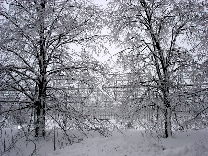
         Computer                     emission

Outlook of the North arm of UTR-2

South arm of UTR-2 in winter time

Observations of carbon RRLs towards Cassiopeia A

The interstellar clouds lying against a
  supernova remnant Cassiopeia A are the
  best studied objects with low frequency
  carbon RRLs. They have been observed in
  wide frequency range from 12 MHz to 1.5
  GHz. Up to ~ 120 MHz RRLs are observed
  in absorption.

Carbon RRLs measured in the direction towards Cas
                A with UTR-2
   20 MHz range – C683 … C696α , C860 …C877β (~30 h)
26 MHz range – C627…C636α, C790…C802β, C904…C917γ,
                 C994…C1009 δ (~500h)
    30MHz range – C599…C606α, C755…C764β (~90 h)
     31 MHz range – C592…C598α, C746…C754β (20 h)

Folded C627…C636 α RRLs measured towards Cas A
                            In our case of very high atom
                               quantum states n>>∆n and
                               adjacent features can be
                               considered as equivalent.
                               Thus, we could fold
                               individual transitions and
                               improve measurement
                               sensitivity considerably.
                               Moreover, such an approach
                               provides more reliable line
                               parameters measurements
                               because different transitions
                               are observed simultaneously
                               with the same antenna and
                               medium conditions.

Interference reduction
Usually spectroscopic observations at UTR-2 are carried out using
   four minute frames, which are stored in computer.
In order to remove hindering signal from processed spectrum we
   subtract from measured autocorrelation function a model of
   interference. It is described by

                                                                  
                                        
                                 iπ ∆ f                         −   
            []
          Ri =
               2A
                  exp −                  cos 2π  f − f  i   1
                                                                     
               r1    
                           ( 2 ln 2) f    o  f d 
                                      2  
                                       d

where R[i] – autocorrelation function of hindering signal, А –
  amplitude of hindering signal , r1 – autocorrelation function point
  number, ∆f – bandwidth of hindering signal, fd – sampling
  frequency fo – frequency of the local oscillator.

Observed and real line intensities

             TB >>TF   (Cas A case)

       ∆ TL         ∆ TL    TCasA + TB 
              =                   
        TC  real  TC  obs  TCasA 

The size of the atoms producing decametric
                    carbon RRLs

For transitions at different n, the size of the atom is given
  by

                          2   −1
           d = 2a0n Z                nm

where a0 = 0.05 nm, the Bohr radius, Z – effective nuclear
  charge of recombining ion, it is equal 1 in our case.

So, for n=1009, d=0.108 mm.

How many levels can be in an atom in space

Alkali and alkaline earth metals like potassium and
  barium have been excited to high quantum levels (up to
  n~1,100) in the laboratory by using tunable dye lasers.
When we take into account the typical conditions of the
  ISM in the Galaxy, the fundamental limit of the highest
  bound state of a Rydberg atom is near n=1,700. These
  are arrived at by estimating the quantum level at which
  the rate of depopulation exceeds the orbital frequency
  of the electron.
But if we take into account the radiation broadening due
  to background radiation in the Galaxy (its brightness
  temperature increases quickly with drop of frequency),
  the maximum quantum level at an atom could be less
  then mentioned above value.

Conclusions

• Study of LF RRLs is important approach of the ISM
  diagnostic.
• In order to obtained high quality LF RRL data we need
  effective instrument.
• Opportunities that will be opened by LOFAR in the
  field are very promising

References

1.   Konovalenko, A. A., Sodin, L. G. The 26.13 MHz absorption line in
     the direction of Cassiopeia A. Nature 294, 135 (1981).
2.   Kantharia, N. G., Anantharamaiah, K. R. & Payne, H. E. Carbon
     recombination lines between 35.5 and 770 MHz toward Cassiopeia
     A. Astrophys. J. 506, 758–772 (1998).
3.   Gordon, M. A., Sorochenko, R. L. Radio Recombination Lines:
     Their Physics and Astronomical Application. , (Kluwer, 2002).
4.   Stepkin, S. V., Konovalenko, A. A. , Kantharia, N. G., & Udaya
     Shankar, N. Radio recombination lines from the largest bound
     atoms in space. Mon. Not. R. Astron. Soc. 374, 852-856 (2007).