Towards aerodynamically equivalent COVID19 1.5 m social distancing for walking and running

Page created by Gabriel Paul

Current Events

English

Like
Share
Embed
Fullscreen
Slides
Download HTML
Download PDF
Abuse

←

→

Page content transcription

If your browser does not render page correctly, please read the page content below

Preprint

Towards aerodynamically equivalent COVID19 1.5 m
social distancing for walking and running
B. Blocken 1,2, F. Malizia 2, T. van Druenen 1, T. Marchal 3
Corresponding author: b.j.e.blocken@tue.nl
1
Building Physics and Services, Department of the Built Environment, Eindhoven University of Technology,
P.O. box 513, 5600 MB Eindhoven, the Netherlands

2
Building Physics Section, Department of Civil Engineering, KU Leuven, Kasteelpark Arenberg 40 - bus 2447,
3001 Leuven, Belgium
3
Ansys Belgium S.A., Centre d'Affaires “Les Collines de Wavre”, Avenue Pasteur 4, 1300, Wavre, Belgium

Abstract
Within a time span of only a few months, the COVID-19 virus has managed to spread to many countries in the
world. Previous research has shown that the spread of this type of viruses can occur effectively by means of
saliva, often in the form of micro-droplets. When a person sneezes, coughs or even exhales, he or she is emitting
small droplets – often too small to see with the naked eye – that can carry the virus. The receiving persons can
be infected by inhaling these droplets, or by getting these droplets on their hands and then touching their face.
That is why during the COVID-19 crisis, countries world-wide have declared – sometimes by law – a “social
distance” of about 1.5 m to be kept between individuals. This is considered important and effective because it is
expected that most of the droplets indeed fall down and reach the floor and/or evaporate before having traveled
a distance of 1.5 m. However, this social distance has been defined for persons that are standing still. It does not
take into account the potential aerodynamic effects introduced by person movement, such as walking fast,
running and cycling. This aerodynamics study investigates whether a first person moving nearby a second person
at 1.5 m distance or beyond could cause droplet transfer to this second person. CFD simulations, previously
validated and calibrated with wind tunnel measurements of droplet movement and evaporation and of airflow
around a runner, are performed of the movement of droplets emitted by an exhaling walking or running person
nearby another walking or running person. External wind is considered absent and different person
configurations are analyzed, side by side, inline and staggered, and the exposure of the second person to the
droplets emitted by the first person is assessed. The results indicate that the largest exposure of the trailing person
to droplets of the leading person for walking and running is obtained when this trailing person is in line behind
the leading person, i.e. positioned in the slipstream. The exposure increases as the distance between leading and
trailing person decreases. This suggests that avoiding substantial droplet exposure in the conditions of this study
and in a way equivalent to the 1.5 m for people standing still can be achieved by one of two actions: either by
avoiding to walk or run in the slipstream of the leading person and keeping the 1.5 m distance in staggered or
side by side arrangement, or by keeping larger social distances, where the distances increase with the walking or
running speed.

Keywords: Social distance; Building physics; Wind engineering; Aerodynamics; Droplet dispersion; Sports

1. Introduction

Studies in medical and other journals have provided a lot of information following the SARS (Severe
Acute Respiratory Syndrome) epidemic that started end of 2002. Seto et al. (2003) investigated the effectiveness
of precautions against droplets and contact in prevention of the transmission of SARS. They performed a control
study in five Hong Kong hospitals, with 241 non-infected and 13 infected staff with documented exposure to 31
index patients with SARS during patient care. Four precautions were considered: using masks, gloves, gowns
and hand-washing. All the participants were monitored for these actions. The 69 staff members that were reported
to use all four measures were not infected, while all infected staff members had omitted at least one measure.
They noted that the practice of droplet precaution and contact precaution is effective to significantly reduce the
risk of infection and they concluded that the infection is transmitted by droplets. Yang et al. (2007) investigated
the size distribution of coughed droplets and of the droplet nuclei by test persons. They found that the total
average size distribution of the droplet nuclei was 0.58–5.42 m, and 82% of droplet nuclei centered in 0.74–
2.12 m. The entire average size distribution of the coughed droplets was 0.62–15.9 m, and the average mode
size was 8.35 m, while the size distribution of the coughed droplets was multimodal with peaks at
approximately 1 m, 2 m, and 8 m. Johnson and Morawska (2009) studied the mechanism of breath aerosol
formation. They analyzed the aerosol size distribution in exhaled breath for normal breathing, varied breath-
holding periods, and contrasting inhalation and exhalation rates. They found that deep exhalation yielded a four-
to sixfold increase in concentration and rapid inhalation a further two- to threefold increase in concentration,
while rapid exhalation had little effect on the measured concentration. Xie et al. (2009) performed experiments
to measure the number and size of respiratory droplets produced from the mouth of healthy persons during talking
and coughing. They found a considerable subject variability and an average size of droplets of about 50 – 100
m using glass slides and a microscope, although smaller droplets were also found using the aerosol spectrometer.
Also many researchers in civil engineering, including building physics and wind engineering, and some
other fields have investigated the transmission of diseases such as SARS by liquid droplets in the air. Zhu et al.
(2004) investigated SARS infection via droplets of coughed saliva by means of experiments. They concluded
that infection can occur when in close contact with SARS patients through coughed saliva droplets. Wang et al.
(2005) also stated that micro-scale liquid droplets could act as the SARS carriers in the air when released from
an infected person by breathing, coughing or sneezing. They developed a model to investigate the effect of the
relative humidity on the movement of these liquid droplets in the air and found that higher relative humidity
could lead to droplets evaporating less quickly and therefore falling faster and reducing the probability of droplet
inhalation. Zhu et al. (2006) studied the transport characteristics of cough droplets in a calm indoor environment.
They found that for the subjects studied and during each individual cough, more than 6.7 mg of saliva was
expelled at speeds of up to 22 m/s during each individual cough and that the saliva droplets could travel further
than 2 m. They also observed that the movement of droplets of 30 m of less was primarily driven by the indoor
airflow patterns rather than gravity due to their small size. Droplets of 50–200 m fell as the flow field weakened
and larger droplets of 300 m and more were more affected by inertia than gravity and did not fall that quickly.
Ai and Melikov (2018) reviewed studies on the airborne spread of expiratory droplet nuclei between the
occupants of indoor environments, with specific focus on the spread of droplet nuclei from mouth/nose to
mouth/nose for non-specific diseases. They indicated that the spread of the nuclei was well investigated under
steady-state conditions and with steady-state Reynolds-averaged Navier-Stokes (RANS) computational fluid
dynamics (CFD) simulations. They indicated that future research is needed in three specific areas: the importance
of the direction of indoor airflow patterns, the dynamics of airborne transmission and the application of CFD
simulations.
As mentioned earlier, it is often assumed that most of the respiratory droplets fall down and reach the
floor and/or evaporate before having traveled a distance of 1.5 m, which is what has inspired the COVID-19
social distance of 1.5 m. However, micro-droplets have very little inertia and when two people are walking or
running in each other’s vicinity, even at 1.5 m distance, due to the airflow patterns and people movements, these
micro-droplets could be transferred from person A to person B due to the airflow patterns generated by the
persons’ movement. This study investigates whether this can be the case To the best of our knowledge, no
previous studies have focused on the potential spread of droplets from a person to another when both are moving
fast, such as in walking fast or running exercises outdoors. More specifically, the objective of this study is to
investigate to what extent the social distance of 1.5 m should be adjusted to provide a similar level of “non-
exposure” to droplets from the mouth of person A to the face of person B as for the case with 1.5 m between two
people standing still and talking to each other. This study employs numerical simulations with CFD, validated
with previously performed wind tunnel experiments by the authors and also wind tunnel experiments published
by other authors in the scientific literature. Unsteady RANS CFD simulations are employed on high-resolution
grids with near-wall cell sizes down to 50 m to also resolve the thin viscous sublayer on the surface of the
persons. This study fits in two of the three specific areas identified by Ai and Melikov: the movement of the
persons creates specific airflow patterns that will influence the dynamic movement of the droplets. In addition,
pseudo-transient CFD simulations are required in order to provide sufficiently accurate representations of the

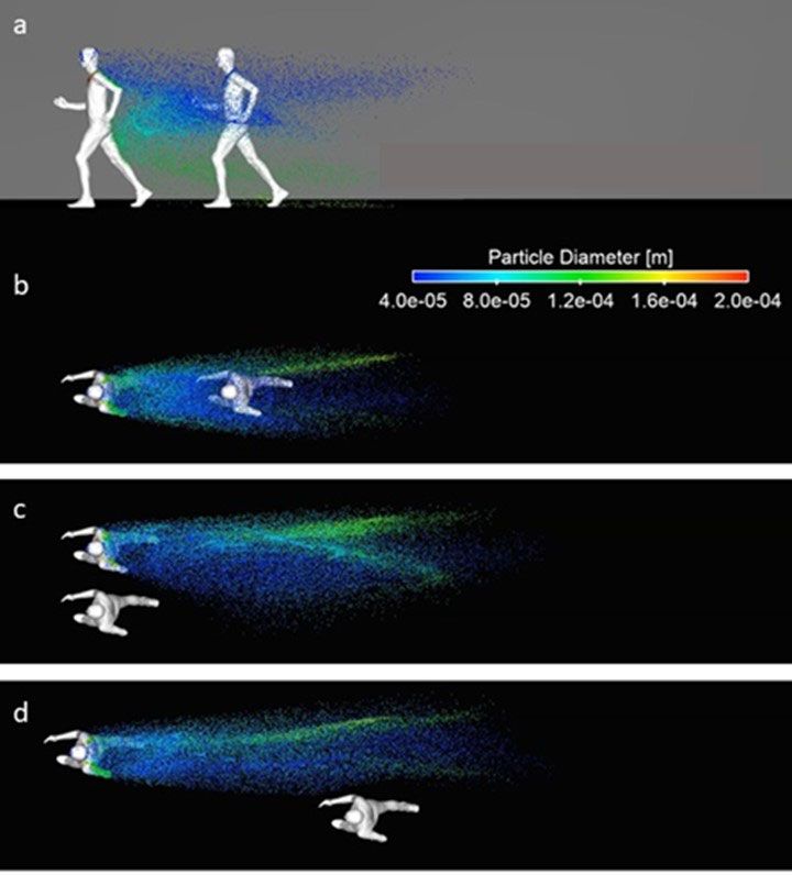
flow field around persons walking fast or running, as has been demonstrated in recent studies for cycling
(Blocken et al. 2018a; 2018b; 2019; Mannion et al. 2019).
The paper is organized as follows. Section 2 presents the validation with the wind tunnel experiments in
two parts, first the validation of the CFD simulations of micro-droplet movement and evaporation and second
the validation of the CFD simulations of the runner geometry that will also be used in the next sections. Section
3 outlines the computational settings and parameters of the CFD simulations. Section 4 shows the research results.
Section 5 (discussion and limitations) and Section 6 (summary and conclusions) conclude the paper.

2. CFD validation study 1: Droplet movement and evaporation

2.1. Wind tunnel measurements

The wind tunnel measurements were described in detail in two earlier studies (Sureshkumar et al. 2008;
Montazeri et al. 2015a), therefore only the main items are mentioned here.
Sureshkumar et al. (2008) studied the evaporative cooling performance of a hollow-cone nozzle spray
system in an open-circuit aeronautical wind-tunnel with a uniform mean wind speed. The wind tunnel had a
cross section of 0.585 m x 0.585 m and a length of 1.9 m (Fig. 1a). The dry bulb temperature (DBT) and wet
bulb temperature (WBT) variations of the air were measured at the inlet plane of the test section, where the
spray nozzle was installed, and the outlet plane, for different air flow conditions and spray characteristics. The
inlet air DBT and WBT were measured by two thermocouples placed upstream of the nozzle. The outlet air
DBT and WBT were measured using 18 thermocouples (Fig. 1b). The air velocity was measured with a
thermal probe installed upstream of the spray nozzle. The mean velocity measurement accuracy was less than
+/-0.05 m/s for air velocity up to 2 m/s and +/-0.2 m/s for air velocity between 2 and 4 m/s. Wetting of the
thermocouples was avoided by a drift eliminator with z-shaped plates placed close to the tunnel outlet to
collect the remaining water droplets in the air flow. The sump water was collected in a separate tank to avoid
mixing of supply and sump water in order to keep the water inlet temperature constant during each set of
experiments. The inlet and outlet water temperatures were measured using two thermocouples upstream of the
nozzle and downstream of the drift eliminator, respectively. Water pressure was also measured by a pressure
gauge upstream of the nozzle.
Four identical nozzles but with different discharge openings of 3, 4, 5 and 5.5 mm were used. Each
nozzle was installed in the middle of the test section (Fig.1a) and designed in a way that the exiting water
forms a hollow-cone sheet disintegrating into droplets. The droplet diameter distribution was determined using
an image-analyzing technique with a measurement accuracy for the mean droplet size was estimated to be +/-
22%. The half-cone angle was measured in still air and reported as a function of nozzle diameter, water
pressure and background wind speed.
The experiments were conducted in April-June in a hot and dry meteorological conditions. The DBT
and relative humidity (RH) ranged between 35 and 45 °C, and 10 and 35%, respectively. The inlet water
temperature varied between 33 and 36 °C. Measurements were conducted for 36 cases; four different nozzle
discharge diameters (i.e. 3, 4, 5 and 5.5 mm), three inlet nozzle gauge pressures (1, 2 and 3 bar) and three
background wind speeds (1, 2 and 3 m/s). The three cases with a nozzle discharge diameter of 4 mm and a
gauge pressure of 3 bar were taken for the present validation study since droplet size distribution data were
also available for these cases. Table 1 summarizes some key parameters.

Fig. 1 (a, b) Wind-tunnel measurement setup with measurement positions in the outlet plane (modified from
Sureshkumar et al. 2008). Dimensions in meter.

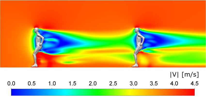
Table 1: Some key parameters of the three cases studied

2.2. CFD simulations

2.2.1. Geometry, grid and boundary conditions

Validation studies of droplet movement and evaporation have been performed earlier by our team members
(Montazeri et al. 2015a; 2015b). Therefore, only the headlines of those studies are reported here. The multi-
phase simulations are performed with the Lagrangian-Eulerian (LE) approach. The computational domain
represented the wind-tunnel test section. The computational grid contained 1,018,725 hexahedral cells (Fig. 2(b))
with a stretching ratio of 1.05 around the nozzle. The grid resolution resulted from a grid-sensitivity analysis
reported in Montazeri et al. (2015a). A uniform mean inlet velocity and a turbulence intensity I of 10% were
imposed, from which the turbulent kinetic energy k and turbulence dissipation rate ε were obtained as in the
equations below where C is a constant (=0.09). The turbulence length scale, l, in this equation is taken as 0.07DH
where DH is the hydraulic diameter of the domain equal to the test section width (= 0.585 m).

A constant temperature and a fixed vapour mass fraction were also imposed at the inlet. The walls of the
computational domain were modelled as adiabatic no-slip walls with zero roughness height kS = 0 in the
standard wall functions (Launder and Spalding 1974). Zero static gauge pressure was applied at the outlet
plane. Special attention is needed for the discrete phase boundary conditions to take the effect of the wind-
tunnel walls into account. More information can be found in Montazeri et al. (2015a; 2015b).

Fig. 2 (a) Computational domain (dimensions in meter). (b) Computational grid (1,018,725 cells).

                                                          4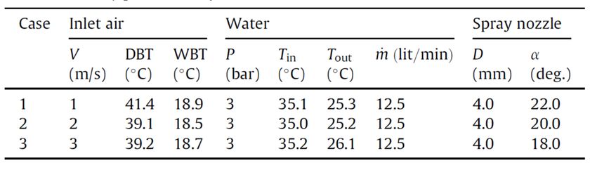

2.2.2. Droplet characteristics

Sureshkumar et al. (2008) used an image-analyzing technique to measure the droplet size distributions. Fig.
3(a) shows the discrete number density distribution for the case that the nozzle diameter and water pressure
were 3 mm and 4 bar, respectively.

Fig. 3. Rosin-Rammler curve fit (solid line) and experimental data of YD (dots).

2.2.3. Solver settings

The 3D steady RANS equations were solved in combination with the realizable k-ε turbulence model by Shih
et al. (1995). The SIMPLE algorithm was used for pressure-velocity coupling, pressure interpolation was
second-order and second-order upwind discretization schemes were used for both the convection terms and the
viscous terms of the equations. For the discrete phase, Lagrangian trajectory simulations were performed. The
discrete phase was modeled to interact with the continuous phase and the discrete phase model source terms
were updated after each continuous phase iteration. The Automated Tracking Scheme Selection was adopted
for the trajectory calculations to be able to switch between higher order lower order tracking schemes, which
can improve the accuracy and stability of the simulations (Subramanian 2013). In this study, trapezoidal and
implicit schemes are used for higher and lower order schemes, respectively. The solution of the droplet
momentum, heat and mass transfer equations are solved in a fully coupled manner.

2.3. CFD validation

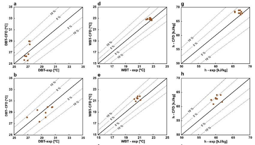
The CFD results from the simulations for the three cases in Table 1 are compared with the wind-tunnel
experiments in terms of the DBT, WBT and specific enthalpy values in the nine measurement points. Note that
the specific enthalpy of moist air, h, can be expressed as:

where hdry_air is the specific enthalpy of dry air (kJ/kgdry_air) given by CpT, where Cp is the specific heat capacity
of air (kJ/kgK). x is the humidity ratio (kgvapour/kgdry_air) and hv the specific enthalpy of water vapour. The
results in Fig. 5 show a good agreement, within 10% for DBT, 5% for WBT and 7% for the specific enthalpy
for all cases. The exact reasons for these deviations are not clear, but they are probably caused by a
combination of limitations of the LE approach and experimental uncertainties. Apart from the LE approach
limitations, the impact of collision of droplets, droplets impingement on solid surfaces and the drift eliminator
on the air flow are not considered into account in this study. Further discussion on these results can be found in
Montazeri et al. (2015a; 2015b). The good agreement obtained in this validation study indicates that droplet
movement and evaporation can be accurately modeled in CFD.

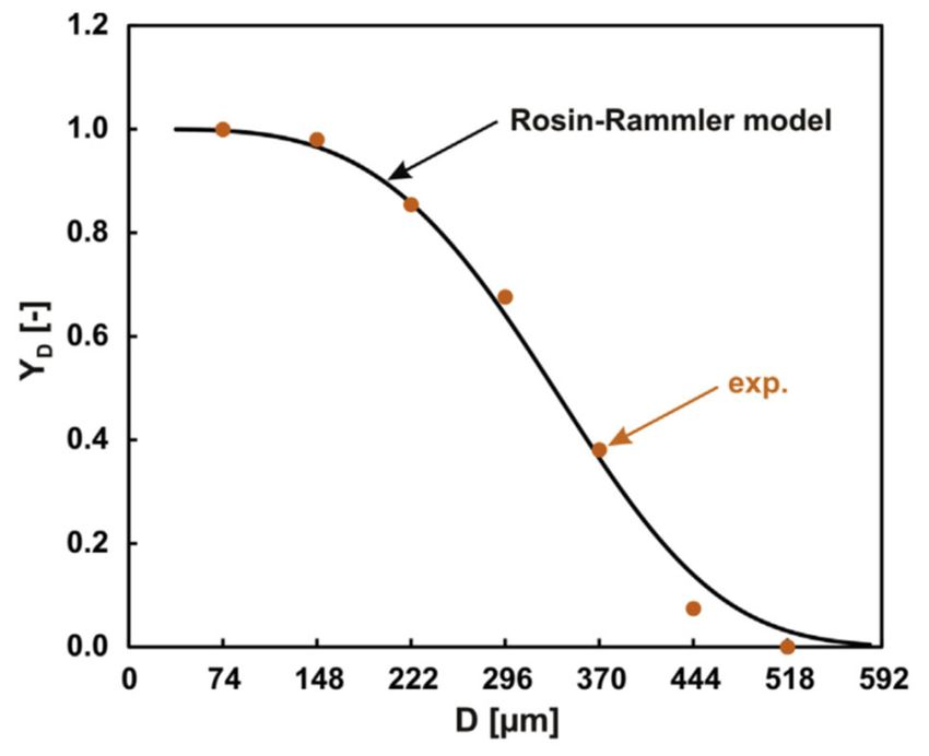
Fig. 5. Comparison of calculated (CFD) and measured (exp. by Sureshkumar et al. (2008)) (a,e,c) DBT, (b,e,f)
WBT and (g,e,i) specific enthalpy for case 1, 2 and 3, respectively.

3. CFD validation study 2: Aerodynamic drag on a runner

3.1. Wind tunnel measurements

A quarter-scale model of a runner was made by CNC cutting (Fig. 6). The geometry of the runner was obtained
by scanning an actual male runner with a height of 186 cm. He was positioned in a fixed running position and
wearing loose-fitting running clothes. The wind tunnel tests were performed in the wind tunnel of Eindhoven
University of Technology. A dedicated set-up with an elevated sharp-edged smooth horizontal plate and
embedded force balance was developed to limit boundary layer development. The drag force on the cyclist was
measured with a force transducer designed specifically for high-accuracy quarter-scale cyclist wind tunnel tests
(Blocken et al. 2018a) with an equipment accuracy of 0.001 N. Data were sampled at 10 Hz for 60 s. Tests
were performed at wind speeds of 15, 20, 25 and 30 m/s, where Reynolds number independence was noted
above 20 m/s. The Reynolds-number independent results were retained and will reported later together with the
CFD results. It was assumed that there is no crosswind, no head wind and no tail wind, therefore the wind
tunnel speed represented the running velocity. Based on these measurements, the repeatability of obtained drag
values was found to be ±0.8%, which corresponds to drag differences of ± 0.3 N for the isolated runner. Drag
measurements were corrected to match the conditions set in the CFD simulations of 101325 Pa, 15°C, 4 m/s
and full geometrical scale. The approach-flow turbulence was 0.3%. The measurement results will be reported
together with the CFD results in the next section.

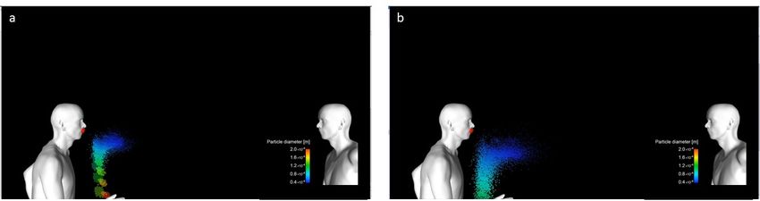
Fig. 6: Runner model on sharp-edged elevated plate in the wind tunnel.

3.2. CFD simulations: computational settings, parameters and validation

The CFD simulations were performed at full scale. The computational geometry of the runner was identical to
that of the wind tunnel model except for the wind tunnel model bottom plate and for the geometrical scale. The
computational domain was a rectangular prism according to best practice guidelines in urban physics and wind
engineering (Franke et al. 2007, Tominaga et al. 2008, Blocken 2015). The blockage ratio was below 5%. The
hybrid hexahedral-polyhedral computational grids were generated based on grid convergence analysis (not
reported here) and on CFD grid generation guidelines (Casey and Wintergerste 2000; Tucker and Mosquera
2001; Franke et al. 2007; Tominaga et al. 2008; Blocken 2015). This analysis indicated the necessity of a wall-
adjacent cell size of 50 micrometer (= 0.05 mm) and 40 layers of prismatic cells near the surfaces of the runner
(Fig. 4). This was required to accurately resolve the thin boundary layer including the viscous sublayer. The
dimensionless wall unit y* had values that were generally below 1 and everywhere below 5. Here, y* was defined
as y* = u*yP/ where u* = Cµ1/4kP1/2. Cµ was a constant (= 0.09) and kP was the turbulent kinetic energy in the
wall-adjacent cell center point P. Note that generally the parameters y+ and u+ were used instead of y* and u*
but that the latter parameters have the advantage that they can also be used to specify grid resolution requirements
at flow field positions where the shear stress is zero, such as stagnation and reattachment points. At these
positions, y+ is zero, irrespective of the local grid resolution yP, and therefore the parameter y+ cannot be used to
specify the grid requirements. The parameter y* however will not be zero because it is based on kP. The grid
convergence analysis also indicated the necessity of a cell size of 0.03 m in the area around the runner. Figure 7
shows the grid resolution on the surface of the runner. The total cell count is about 6x106 cells.

Fig. 7: High-resolution computational grid on the runner and in the vertical centerplane. Total cell count is
about 6x106 cells.

At the inlet, a uniform velocity of 4 m/s was imposed, which represents a running velocity of 14.4 km/h.
As in the wind tunnel tests, it was assumed that there is no crosswind, no head wind and no tail wind. At the
outlet, zero static gauge pressure was set. The bottom, side and top surfaces of the domain were slip walls. The
inlet turbulence intensity had to be set to 0.5% to obtain the same approach-flow values in the region directly
upstream of the motorcycle as in the wind tunnel.
The 3D unsteady Reynolds-averaged Navier-Stokes (URANS) equations were solved with the Shear
Stress Transport (SST) k- model (Menter 1994). Pressure-velocity coupling was taken care of by the coupled
algorithm with pseudo-transient under-relaxation and a pseudo-transient time step of 0.01 s. Pressure
interpolation was second order, gradient interpolation was performed with the Green-Gauss node based scheme
and second-order upwind discretization schemes were used for both the convection terms and the viscous terms
of the governing equations. Simulations were run for a total of 5000 pseudo-transient time steps and averaging
of the results was performed for the last 4000 time steps. Tests confirmed that the total number of 5000 was
sufficient to obtain stationary results.
The aerodynamic drag area of the runner was computed to be 0.301 m² and the measured value was 0.303
m² which is a very close agreement. Combined with previous successful CFD validation studies of athletes
(cyclists) with wind tunnel measurements (Blocken et al. 2018a; 2018b; 2019; Mannion et al. 2018), it was
decided to retain the current computational settings and parameters for the study in the next section.

4. CFD study of droplet dispersion around two walkers or two runners

4.1. CFD simulations: computational settings and parameters

The two validation studies support the simulations of the airflow and droplet dispersion around the two
walkers/runners. Different configurations of walkers/runners were considered: side by side at a distance of 1 m,
in line at distances of 1.5 m, 3 m, and beyond in steps of 1.5 m, and staggered at a lateral distance of 1 m and a
distance in the direction of movement of 1.5 m, 3 m, and beyond in steps of 1.5 m. Also a reference configuration
with two people standing still at 1.5 m “standard social distance” was considered. The CFD simulations were
again performed at full scale. The computational geometry of the two walkers/runners was identical to that in
Section 3. The computational domain and computational grid were based on best practice guidelines and a
similarly high grid resolution of 50 micrometer (= 0.05 mm) and 40 layers of prismatic cells were applied near
the surfaces of the runner. Figure 8 and 9 display parts of the computational grid. The total cell count was about
9x106 cells.

Fig. 8: Computational grid on the surfaces of the two runners, with specific refinement near the mouth opening.
Total cell count is about 9x106 cells.

Fig. 9: Computational grid in vertical centerplane. Total cell count is about 9x106 cells.

The computational settings and parameters were similar to those in Section 3 apart from the following
changes. The inlet velocity represented the walking/running velocity and was set at 1.11 m/s (= 4 km/h) for
walking (fast) and 4 m/s (= 14.4 km/h) for running. There is no head wind, tail wind or cross-wind. The exhaling
velocity was 2.5 m/s relative to the movement of the walker/runner, representing moderately deep breathing.
Saliva droplets were represented by water and released at a total flow rate of 1x10-14 mg/s with a Rosin-Rammler
droplet distribution with minimum diameter of 40 m, an average diameter of 80 m and a maximum diameter
of 200 m, in line with the values by Zhu et al. (2006) and Xie et al. (2009).

4.2. CFD simulations: results

The results are presented in the form of graphs and in a binary mode (whether droplets reach the second
person or not). Figure 10 shows the contours of airspeed in the vertical centerplane for two persons running in
line at a distance of 4.5 m, clearly indicating the wake (slipstream) behind each of the runners. Figure 11 shows
two snapshots for the case of two people standing still at 1.5 m distance. It shows droplets being exhaled at two
different moments in time, with the larger droplets falling down faster, as expected. Figure 11 Figure 12 shows
snapshots of a number of the simulations where the droplets exhaled by the leading runner are visualized. Figure
12a and b represent the two runners in line at a speed of 4 m/s and a separation distance of 1.5 m. The smaller
fraction of the droplets exhaled by the leading runner, because of their lower inertia, do not move along with the
leading runner but are entrained in his/her wake. The trailing runner present in this wake will be exposed to these
droplets. Figure 12c is a similar figure for runners side by side. The droplets again are entrained in the wake of
the exhaling runner and in this case do not reach the body of the second runner. Figure 12d finally displays the
situation for two runners in staggered formation at a distance of 3 m in the moving direction. Again, the droplets
are entrained in the wake and the trailing runner is not exposed to these droplets.

Fig. 10: Contours of air speed in the vertical centerplane when running at 4.5 m distance at 4 m/s.

Fig. 11: Particles released for two people at 1.5 m distance at different points in time.

Fig. 12: Droplet spreading when running at a speed of 14.4 km/h when (a,b) running behind each other; (c)
side-by-side; (d) in staggered arrangement.

                                                          10

5. Discussion and limitations

The simulations presented in Section 4 along with all simulations performed lead to the conclusion that for the
runners geometries, walking/running velocities, absence of external wind and the exhaling velocity and droplet
spectrum included in these simulations, the largest exposure to droplets systematically occurs when the trailing
runner is positioned in the slipstream of the leading runner. The smaller the distance between the runners, the
larger the fraction of droplets to which the trailing runner is exposed. Analyzing the results of all the simulations,
the main conclusion is that substantial droplet exposure occurs when the trailing runner is positioned in the
slipstream of the leading runner, up to a distance between both that depends on the traveling speed. For walking
at 4 km/h a distance of about 5 m leads to no droplets reaching the upper torso of the trailing runner. For running
at 14.4 km/h this distance is about 10 m. This implies that if one assumes that 1.5 m is a social distance to be
maintained for two people standing still, this value would have to be increased to 5 m or 10 m for slipstream
walking fast and slipstream running, respectively, to have a roughly equivalent non-exposure to droplets as two
people standing still at 1.5 m distance. This leads to the tentative advice to walkers and cyclists that if they wish
to run behind and/or overtake other walkers and runners with regard for social distance, they can do so by moving
outside the slipstream into staggered formation when having reached this distance of about 5 m and 10 m for
walking fast and running, respectively.
The study is subjected to a number of limitations that will give rise for further work. Further work will
consider the effect of head wind, tail wind and cross-wind. Cross-wind will cause the slipstream to be not straight
but obliquely positioned behind the runners, and while it is expected that also in this case the droplets will mainly
remain entrained in the slipstream, this should be confirmed by future simulations. External wind will also
increase the turbulence intensity and might cause stronger mixing of the droplets in the slipstream, and potentially
also allow a small fraction droplets to escape the slipstream. Further work can also consider walkers and runners
at different velocities overtaking each other and runners crossing each other. Finally, additional droplet spectra
can be considered containing smaller but also larger droplets, as produced by coughing and sneezing. In the
present study, it was decided to focus on droplets characteristics representative of exhaling and coughing, rather
than sneezing. The larger fraction of large droplets produced by sneezing will more rapidly fall down to the
ground yielding a lower exposure risk.

6. Summary and conclusions

Within a time span of only a few months, the COVID-19 virus has managed to spread to many countries in the
world. Previous research has shown that the spread of this type of viruses can occur effectively by means of
saliva, often in the form of micro-droplets. When a person sneezes, coughs or even exhales, he or she is emitting
small droplets – often too small to see with the naked eye – that can carry the virus. The receiving persons can
be infected by inhaling these droplets, or by getting these droplets on their hands and then touching their face.
That is why during the COVID-19 crisis, countries world-wide have declared – sometimes by law – a “social
distance” of about 1.5 m to be kept between individuals. This is considered important and effective because it is
expected that most of the droplets indeed fall down and reach the floor and/or evaporate before having traveled
a distance of 1.5 m. However, this social distance has been defined for persons that are standing still. It does not
take into account the aerodynamic effects introduced by person movement, such as walking fast, running and
cycling. This aerodynamics study investigates whether a first person moving nearby a second person at 1.5 m
distance or beyond could cause droplet transfer to this second person. CFD simulations, previously validated
with wind tunnel measurements of droplet movement and evaporation and of airflow around a runner, are
performed of the movement of droplets emitted by an exhaling walking or running person nearby another
walking or running person. External wind was considered absent and different person configurations are analyzed,
side by side, inline and staggered, and the exposure of the second person to the droplets emitted by the first
person is assessed. The results indicate that the largest exposure of the trailing person to droplets for walking
and running is obtained when this person is in line and with leading person and positioned in the slipstream of
this person. Exposure increases as the distance between leading and trailing person decreases. This suggests that
avoiding substantial droplet exposure in the conditions of this study can be achieved by one of two actions: either
by avoiding to walk or run in the slipstream of the leading person or by keeping larger social distances, where
the distances increase with the walking or running speed. The equivalent social distance for walking and running
in the slipstream is defined as the distance that should be kept between the leading and trailing walker/runner to
avoid substantial exposure to slipstream droplets, similar to the case where two people are standing still at 1.5 m
distance. In the absence of head wind, tail wind and cross-wind, for walking fast at 4 km/h this distance is about
5 m and for running at 14.4 km/h this distance is about 10 m. Further work should consider the effect of head
wind, tail wind and cross-wind, and different droplet spectra.

References

Ai ZT, Melikov AK. 2018. Airborne spread of expiratory droplet nuclei between the occupants of indoor
environments: A review. Indoor Air 28: 500-524.
Blocken B, van Druenen T, Toparlar Y, Malizia F, Mannion P, Andrianne T, Marchal T, Maas GJ, Diepens J.
2018a. Aerodynamic drag in cycling pelotons: new insights by CFD simulation and wind tunnel testing.
Journal of Wind Engineering & Industrial Aerodynamics 179: 319-337.
Blocken B, van Druenen T, Toparlar Y, Andrianne T. 2018b. Aerodynamic analysis of different cyclist hill
descent positions. Journal of Wind Engineering & Industrial Aerodynamics 181: 27-45.
Blocken B, van Druenen T, Toparlar Y, Andrianne T. 2019. CFD analysis of an exceptional cyclist sprint position.
Sports Engineering 22:10.
Blocken B. 2015. Computational Fluid Dynamics for urban physics: Importance, scales, possibilities, limitations
and ten tips and tricks towards accurate and reliable simulations. Build Environ 91:219–245
Casey M, Wintergerste T. 2000. Best Practice Guidelines. ERCOFTAC Special Interest Group on ‘‘Quality and
Trust in Industrial CFD’’. ERCOFTAC
Franke J, Hellsten A, Schlünzen H, Carissimo B. 2007. Best practice guideline for the CFD simulation of flows
in the urban environment, COST action 732
Johnson GR, Morawska L. 2009. The mechanism of breath aerosol formation. Journal of Aerosol Medicine and
Pulmonary Drug Delivery 22(3): 229-237.
Launder BE, Spalding DB. 1974. The numerical computation of turbulent flows. Comput Methods Appl Mech
Eng 3:269-289.
Mannion P, Toparlar Y, Blocken B, Hajdukiewicz M, Andrianne T, Clifford E. 2019. Impact of pilot and stoker
torso angles in tandem para-cycling aerodynamics. Sports Engineering 22: 3.
Menter FR. 1994. Two-equation eddy-viscosity turbulence models for engineering applications. AIAA Journal
32(8): 1598–1605
Montazeri H, Blocken B, Hensen JLM. 2015a. CFD analysis of the impact of physical parameters on evaporative
cooling by a mist spray system. Applied Thermal Engineering 75: 608-622.
Montazeri H, Blocken B, Hensen JLM. 2015b. Evaporative cooling by water spray systems: CFD simulation,
experimental validation and sensitivity analysis. Building and Environment 83: 129-141.
Rosin P, Rammler E. 1933. The laws governing the fineness of powdered coal. J Inst Fuel 31: 29-36.
Seto WH, Tsang D, Yung RWH, Ching TY, Ng TK, Ho M, Ho LM, Peiris JSM. 2003. Effectiveness of
precautions against droplets and contact in prevention of nosocomial transmission of severe acute respiratory
syndrome (SARS). Lancet 361(9368): 1519-1520.
Shih T-H, Liou WW, Shabbir A, Yang Z, Zhu J. 1995. A new k-ε eddy viscosity model for high Reynolds
number turbulent flows. Computer Fluids 24: 227-238.
Subramaniam S. 2013. Lagrangian-Eulerian methods for multiphase flows. Prog Energy Combust Sci 39: 215-
245.
Sureshkumar R, Kale SR, Dhar PL. 2008. Heat and mass transfer processes between a water spray and ambient
air - I. Experimental data. Applied Thermal Engineering 28: 349-360.
Tominaga Y, Mochida A, Yoshie R, Kataoka H, Nozu T, Yoshikawa M, Shirasawa T. 2008. AIJ guidelines for
practical applications of CFD to pedestrian wind environment around buildings. J Wind Eng Ind Aerodyn
96:1749–1761
Tucker P, Mosquera A. 2001. NAFEMS introduction to grid and mesh generation for CFD. NAFEMS CFD
Work. Group.
Wang B, Zhang A, Sun JL, Liu YH, Hu J, Xu LX. 2005. Study of SARS transmission via liquid droplets in air.
Journal of Biomechanical Engineering – Transactions of the ASME 127(1): 32-38.
Xie X, Li Y, Sun H, Liu L. 2009. Exhaled droplets due to talking and coughing. J. R. Soc. Interface 6: 703-714.
Yang S, Lee GWM, Chen CM, Wu CC, Yu KP. 2007. The size and concentration of droplets generated by
coughing in human subjects. Journal of Aerosol Medecine 20(4): 484-494.
Zhu S, Kato S, Yang JH. 2006. Study on transport characteristics of saliva droplets produced by coughing in a
calm indoor environment. Building and Environment 41: 1691-1702.
Zhu SW, Kato S, Yang JH. 2004. Investigation of SARS infection via droplets of coughed saliva. Built
Environment and Public Health, Proceedings. 2nd International Conference on Built Environment and Public
Health (BEPH 2004), pp. 341-354.

You can also read