Fast Magnetic Reconnection induced by Resistivity Gradients in 2D Magnetohydrodynamics
←
→
Page content transcription
If your browser does not render page correctly, please read the page content below
Fast Magnetic Reconnection induced by Resistivity Gradients in 2D Magnetohydrodynamics

                                                    Fast Magnetic Reconnection induced by Resistivity Gradients in 2D
                                                    Magnetohydrodynamics
                                                                Shan-Chang Lin,1, a) Yi-Hsin Liu,1 and Xiaocan Li1
                                                                Dartmouth College, Hanover, NH 03750
                                                                (Dated: 17 September 2021)
                                                                Using 2-dimensional (2D) magnetohydrodynamics (MHD) simulations, we show that Petschek-type magnetic recon-
                                                                nection can be induced using a simple resistivity gradient in the reconnection outflow direction, revealing the key
                                                                ingredient of steady fast reconnection in the collisional limit. We find that the diffusion region self-adjusts its half-
                                                                length to fit the given gradient scale of resistivity. The induced reconnection x-line and flow stagnation point always
arXiv:2109.07526v1 [physics.plasm-ph] 15 Sep 2021

                                                                reside within the resistivity transition region closer to the higher resistivity end. The opening of one exhaust by this re-
                                                                sistivity gradient will lead to the opening of the other exhaust located on the other side of the x-line, within the region of
                                                                uniform resistivity. Potential applications of this setup to reconnection-based thrusters and solar spicules are discussed.
                                                                In a separate set of numerical experiments, we explore the maximum plausible reconnection rate using a large and spa-
                                                                tially localized resistivity right at the x-line. Interestingly, the resulting current density at the x-line drops significantly
                                                                so that the normalized reconnection rate remains bounded by the value ' 0.2, consistent with the theoretical prediction.

                                                    I.   INTRODUCTION                                                        magnetic fields near the end of the diffusion region, which
                                                                                                                             is critical in supporting the open geometry of the Petschek
                                                       Magnetic reconnection is a ubiquitous phenomenon in                   solution. Kulsrud further pointed out the importance of the
                                                    plasma systems that efficiently converts magnetic energy to              resistivity gradient (in the outflow direction) between the x-
                                                    plasma kinetic energy. In astrophysical environments, obser-             line and the end of the diffusion region. The fact that a stable
                                                    vations suggest that magnetic reconnection is the driver of so-          Petschek open geometry can be realized in 2D MHD simu-
                                                    lar flares [e.g., Ref. ? ] and magnetospheric substorms [e.g.,           lations with a localized resistivity at the x-line supports this
                                                    Ref. ? ]. Particles accelerated by magnetotail reconnection              idea? .
                                                    can also be responsible for the generation of aurora borealis               In this work, we demonstrate that a stable Petschek-type
                                                    and aurora australis [e.g., Ref. ? and references therein].              reconnection can be realized by imposing the resistivity that
                                                       Sweet-Parker model? ? and Petschek model? are the two                 has a simple one-dimensional (1D) hyperbolic tangent profile
                                                    most famous classical reconnection models proposed using                 varying along the outflow direction. This result is consistent
                                                    the resistive-MHD framework. Reconnection in the Sweet-                  with the finding of Baty et. al.? , where only half of a lo-
                                                    Parker model develops an elongated diffusion region and                  calized resistivity is used in MHD simulations. In this work,
                                                    has a much smaller reconnection rate compared to that of                 we further show that the resistivity gradient in the outflow
                                                    the Petschek model. While the generalized Sweet-Parker                   direction, not in the inflow direction, is the key to inducing
                                                    model shows agreements with experiments? in the collisional              Petschek-type reconnection in 2D resistive-MHD. This is also
                                                    regime, its reconnection rate is many order of magnitude                 consistent with the result of Yan et. al.? , where they localized
                                                    lower in comparison to that inferred by the energy release               resistivity in the outflow direction only. With a hyperbolic
                                                    time-scale of solar flares? .                                            resistivity profile, we can change the transition region length-
                                                       On the other hand, reconnection in Petschek’s model has a             scale and we find that the reconnection diffusion region will
                                                    short (localized) diffusion region and the outflow is bounded            self-adjust its length so that half of the diffusion region just
                                                    by a pair of standing slow mode shocks. In this reconnec-                fits into this resistive transition region, not longer nor shorter.
                                                    tion geometry, not only the diffusion region thickness is on             The x-line and the flow stagnation point always reside within
                                                    the microscopic scale, but also its length. This is in sharp             this transition region near the high resistivity end. This find-
                                                    contrast to the system-size long diffusion region length in the          ing further supports Kulsrud’s idea? . We also show that the
                                                    Sweet-Parker model. The resulting larger diffusion region as-            averaged-equation method proposed by Baty et. al.? can, in
                                                    pect ratio corresponds to a faster rate, which is fast enough            certain limits, quantitatively predict the spatial profiles of crit-
                                                    to explain the time-scale of solar flare observations and ge-            ical quantities, including the reconnected magnetic field, the
                                                    omagnetic substorms. However, numerical simulations show                 outflow speed, and the reconnection layer thickness. Over-
                                                    that Petschek reconnection can not form in two-dimensional               all, we find that the reconnection rate is determined by both
                                                    resistive-MHD simulations if the resistivity is uniform? ? .             this transition region length and the resistivity value at the
                                                    Such systems appear to lack any mechanism that shortens (lo-             x-line. However, if the background resistivity is too high to
                                                    calizes) the diffusion region length. To explain this result,            have a clear separation between the slow shock transitions
                                                    Kulsrud? suggested that uniform resistivity can not sustain              that bound the outflow exhaust, then the excessive resistive-
                                                    the magnitude of reconnected (normal to the current sheet)               diffusion therein can reduce the reconnection rate. With this
                                                                                                                             understanding in mind, we go back to study Petschek-type re-
                                                                                                                             connection using a two-dimensional (2D) localized resistivity
                                                                                                                             of different peak strength. Interestingly, we find that the cur-
                                                    a) Electronic   mail: shan-chang.lin.gr@dartmouth.edu                    rent density (J) right at the x-line can drop significantly when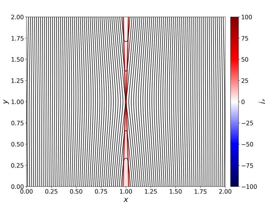
Fast Magnetic Reconnection induced by Resistivity Gradients in 2D Magnetohydrodynamics 2
a large localized resistivity (η) is imposed. The resulting max- free current sheet, described by
imum plausible normalized reconnection rate (ηJ) is around
0.2, likely being constrained by the force-balance upstream ~B = B0 tanh x − xc ŷ + B0 sech x − xc ẑ, (5)
of the diffusion region? ; i.e., the diffusion region physics ap- λ λ
pears to play a passive role and is forced to match this value. where B0 is the magnitude of the anti-parallel magnetic field,
This paper is organized in the following way. The simu- λ is the current sheet half-width and xc is the x-location of the
lation setup and one of the reconnection simulations with a current sheet. We use B0 = 1, λ = 0.04, xc = 1, and initial
hyperbolic tangent resistivity profile are described in section β = p/(B2 /2µ) = 0.1 in all simulations and let simulations
II. In section III, we explain how resistivity-gradient helps evolve to quasi-steady states. The Alfvén speed based on the
maintain reconnected magnetic field, realizing Petschek-type reconnecting magnetic field B0 and the background density
reconnection, as originally proposed by Kulsrud? . We inves- n0 = 1 is therefore VA = 1 in our unit. The simulation domain
tigate the details of the resistive-MHD simulations in section in both the x- and y-directions is from 0 to 2. The resolution
IV A by performing a scaling study using the simple hyper- is 2/512 ∼ 4 × 10⁻³ unless otherwise mentioned. The con-
bolic tangent resistivity profile where we change the transition clusion discussed in this paper do not change with an initial
region length-scale and the background value of the resistivity. Harris sheet configuration (not shown). Especially, the recon-
In section IV B, we study the reconnection rates in simulations nection rate in the nonlinear stage is not sensitive to the choice
using exponentially localized resistivity. In particular, we ex- of the force-free current sheets versus Harris sheets.
amine how the system responds if one dramatically increases We apply a hyperbolic tangent resistivity profile varying in
the resistivity right at the x-line. Finally, we summarize and the y-direction,
discuss the implication and application of this work in sec-
tion V. In the appendix, we briefly summarize the theoretical y−1
ηtanh (y) = 0.5η1 1 − tanh + η2 , (6)
framework by Baty et. al.? that predicts key quantities within lη
the reconnection layer; for a given resistivity profile one can
where lη is the resistivity gradient scale. Equation 6 gives
solve for the outflow speed, the half-width of the reconnec-
asymptotic η = η1 + η2 at y < 1 (i.e., the lower half-plane
tion layer, and the reconnected (normal) magnetic fields. This
in Fig. 1(a) and other similar figures) and η = η2 at y > 1
prediction is compared with our simulation results.
(i.e., the upper half-plane). Simulations show asymmetric
Petschek-type reconnection similar to the results of Baty et.
al.? , in which they used a localized resistivity profile in the
II. MHD SIMULATION WITH A HYPERBOLIC TANGENT
upper half-plane and a uniform resistivity in the lower half-
RESISTIVITY PROFILE
plane. In their simulations, the upper and lower half-planes
are connected by a sharp step-like transition.
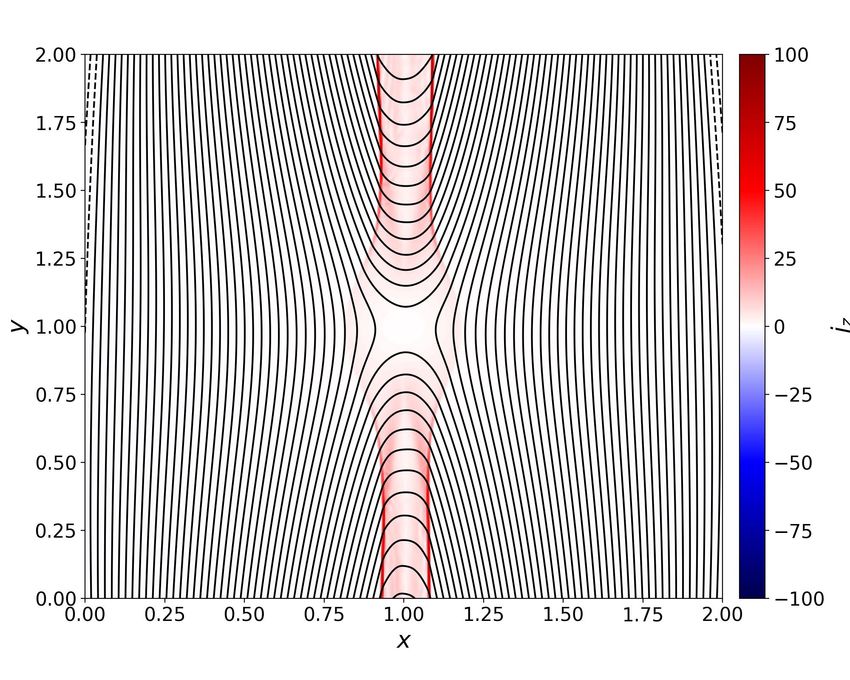
We use Athena? , a grid-based MHD code, to simulate mag- Figure 1 shows a representative run with the hyperbolic tan-
netic reconnection in resistive MHD. The governing equations gent η-profile. The asymptotic resistivity at the upper half-
are plane is 2 × 10⁻⁴ , and that at the lower half-plane is 1 × 10⁻³
with the transition length scale lη = 0.05 (i.e., Run T 1 in Ta-
∂t ρ + ∇ · (ρ~v) = 0 (1) ble I). Panel (a) shows the current density in the z-direction
B2 Jz . The dashed curve in figure 1(a) marks the boundary of one
∂t (ρ~v) + ∇ · [ρ~v~v − ~B~B + (p + )I] = 0 (2) side of the current sheet predicted by the averaged-equations
2
B2 for the given resistivity profile (discussed in Appendix A).
∂t e + ∇ · [(e + p + )~v − ~B(~B ·~v)] = ∇ · (~B × η J)
~ (3) Figure 1(b) shows the cut of the outflow speed. Figure 1(c)
2 shows the cut of the reconnected field. Both panels show the
∂t ~B − ∇ × [~v × ~B − η J]
~ = 0, (4) simulation results (blue solid curve), those predicted by the
averaged-equations (orange dashed curve), and resistivity η
where the energy density e = p/(γ − 1) + ρv2 /2 + B2 /2µ, profiles (red solid curve). The predictions of the averaged-
and the current density J~ = (1/µ)∇ × ~B. The ratio of spe- equations agree reasonably well with this run. The deviation
cific heats γ = 5/3 and η is the resistivity. The permeability of Bx between the averaged-equations solution and the simu-
µ is set to one in code unit. Athena is written based on the lation is larger at the lower-half plane, where η is larger. We
finite-volume method (that solves hyperbolic equations) with will discuss this effect in section IV A. The reconnection rate
the higher-order Godunov methods and the constrained trans- of this case is roughly 0.04 in simulation and 0.07 predicted
port implemented to ensure the divergence-free condition on by the averaged-equations.
the magnetic field. Mass density, momentum, and energy are Interestingly, it appears that the reconnection layer adjusts
solved at the center of grid points, while the magnetic field is itself so that the η-transition region turns to the upper-half of
solved at the center of the grid surfaces. the diffusion region, with both the x-line and flow stagnation
All simulations in this paper are in 2D. The outflowing point locate near the high-η end (see Fig. 1(b) and (c)) and
(zero-gradient) boundary condition with four ghost cells is the upward outflow reaches the plateau at the low-η end (see
used to avoid the saturation due to the flux pileup at outflow Fig. 1(b)). Both exhausts are bounded by slow shocks, and
regions. Importantly, this boundary better allows the system the shock transition region is thinner in the upper-half plane
to evolve into a steady-state. The initial condition is a force- because of the lower resistivity, as expected.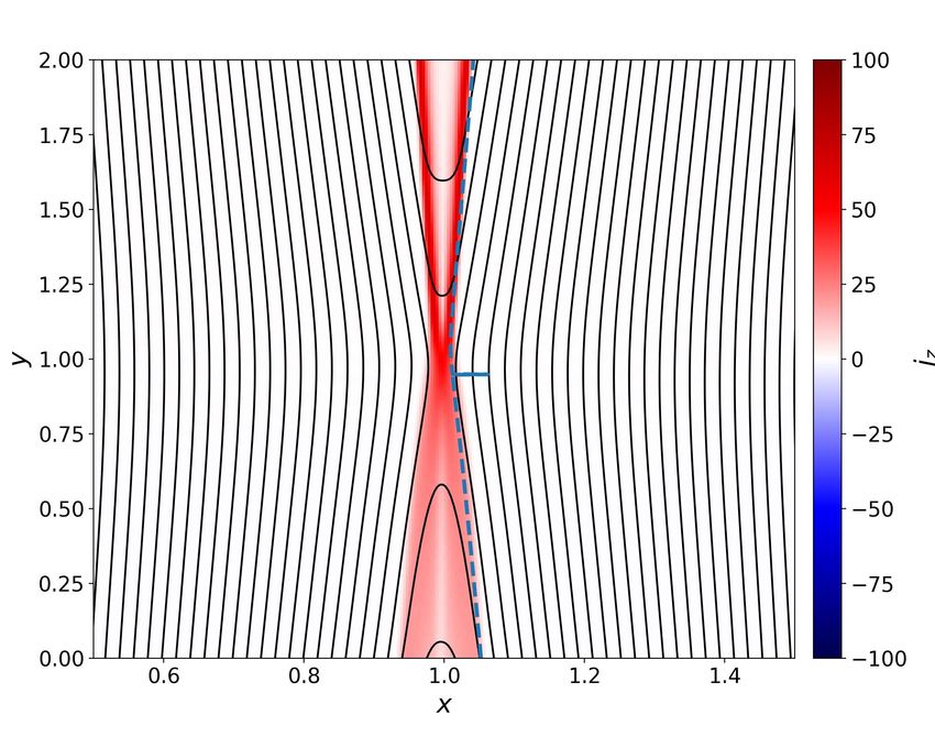
Fast Magnetic Reconnection induced by Resistivity Gradients in 2D Magnetohydrodynamics                                                             3

 (a)                                               (b)                                              (c)
   2                                        100 1                                                 0.2
                                                             η                                                η                               10
                                                                     s                                                x

 y1                                         0       0                                             0.0                                         η

                                                   -1                                            -0.2                                         2
   0                                        -100         0               1                2               0               1               2
       0.6           1.0           1.4                                   y                                                y
                      x

FIG. 1. (Run T 1) (a) The current density Jz under a hyperbolic resistivity profile. The contours of the flux function are shown in black. The
blue dashed curve marks the layer boundary predicted by the averaged-equations in Appendix A. (b) The outflow speed vy cut at the symmetric
line x = 1 in simulation (blue solid line) and that predicted by the averaged-equations (orange dashed line). For reference, the resistivity η is
plotted as the red line. The flow stagnation point is labeled as “s” on the η profile to show its relative position to the η-transition region. (c)
The normal magnetic fields Bx cut at x = 1 in simulation (blue solid line) and that predicted by the averaged-equations (orange dashed line).
The position of the x-line is labeled as “x” on the η-profile.

III. THE ROLE OF RESISTIVITY GRADIENT IN                                     size. By integrating the induction equation from the outflow
PETSCHEK MODEL                                                               symmetry line to the inflow edge of the diffusion region, one
                                                                             can obtain
   Kulsrud? suggested that the reconnected (normal) mag-
                                                                                              ∂ Bx

                                                                                                                       2ηyB0
netic fields immediately downstream of the diffusion region                               a          ≤ ah−vy ∂y Bx i +       ,          (8)
                                                                                               ∂t                       L2
are removed by the advection, but can be replenished by the
reconnecting magnetic field "rotated" into the normal (x-) di-               where a(y) is the width of the diffusion region. In the steady
rection by resistivity gradient within the diffusion region. For             state, ∂ Bx /∂t = 0. At the end of the diffusion region, the
Petschek-type reconnection, if the resistivity is uniform, this              first term on the right hand side scales as −aVA Bx /L0 , where
advective loss will be higher than the generation if the diffu-              VA is the Alfvénic outflow speed and L0 is the half-length of
sion length is not on the order of system size. Therefore, the               the diffusion region. Consequentially, equation (8) then gives
normal magnetic field decreases with time, causing the diffu-                −aVA Bx /L0 + 2ηB0 L0 /L2 ≥ 0. To proceed further, one ap-
sion region to extend to the system size. If there is a resistivity          plies the inflow speed vi = (VA η/L0 )1/2 of the Sweet-Parker
gradient along the outflow direction, it provides an additional              solution? ? based on a diffusion length L0 , the flux conserva-
source to generate the normal magnetic field, opening up the                 tion VA Bx = vi B0 , and the mass√conservation VA a = vi L0 to this
outflow geometry. We will briefly discuss the essence of this                inequality, obtaining L0 ≥ L/ 2. This result suggests that a
argument in the following.                                                   plausible steady-state solution exists only when the diffusion
   If the resistivity is uniform, the x-component of the induc-              length extend to the system size.
tion equation (Eq. (4)) can be expressed as                                     In contrast, if there is a resistivity gradient, the x-
                                         2                                  component of the induction equation becomes
                                          ∂ Bx ∂ 2 Bx

    ∂ Bx                    ~
         = −(~v · ∇)Bx + (B · ∇)vx + η          +           , (7)               ∂ Bx
                                                                                                                     2
                                                                                                                       ∂ Bx ∂ 2 Bx

     ∂t                                    ∂ x2     ∂ y2                                                ~
                                                                                      = −(~v · ∇)Bx + (B · ∇)vx + η          +         −
                                                                                 ∂t                                     ∂ x2    ∂ y2
assuming the plasma around the diffusion region is incom-
                                                                                                                    ∂ η ∂ By ∂ Bx
pressible (i.e., consistent with the simulation results in this                                                                −         . (9)
paper). The first term on the right hand side is the down-                                                          ∂y ∂x          ∂y
swiping term which removes the normal magnetic fields at the                 Since ∂x By  ∂y Bx in the current layer geometry, the last
outflow. Since vx vanishes along the outflow symmetry line,                  term on the right hand side can be approximated as '
−~v · ∇Bx ≈ −vy ∂y Bx . The second term on the right hand side               −(∂y η)(∂x By ) and this term is positive if η is stronger at the
is negative in reconnection geometry, thus Kulsrud? removed                  x-line (i.e., ∂y η < 0 for y > 1). Therefore, this resistivity gra-
this term and turned the equal sign “=” to inequality “≤” in                 dient acts as an additional source to supply the normal mag-
Eq. (7). The resistive term can be approximated as η∂x2 Bx =                 netic field at the outflow, supporting a shorter current sheet
−η∂x ∂y By because ∂x2 Bx  ∂y2 Bx in a typical reconnection ge-             length L0 . The observed open-geometry induced by the sim-
ometry (i.e., low diffusion region aspect ratio) and ∇ · ~B = 0              ple resistivity gradient in our simulations supports this idea.
is used. It was further assumed that By = B0 (1 − y2 /L2 ) along                Note that this argument also works with a current-
the inflow edge of the diffusion region, where L is the system               dependent resistivity η(Jz ) if resistivity can be enhanced by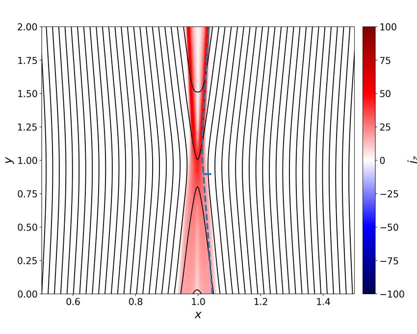
Fast Magnetic Reconnection induced by Resistivity Gradients in 2D Magnetohydrodynamics                                                                                4

the local current density, i.e., ∂Jz η > 0. In this situation,             (a) 2                                       100 (b)
                                                                                                                                                                  10
using the chain rule the last term of Eq. (9) then becomes                                                                0.75           η    s
' −(∂Jz η)(∂y Jz )(∂x By ), that can be positive if the outflows                                                                               x
were to be opened up, which requires ∂y Jz < 0 for y > 1. i.e.,                y1                                      0       0                                  η
this additional supply of Bx can be consistent with an opening
geometry. This prompted the research on the current-driven
                                                                                                                          -0.75
anamolous resistivity? ? ? ? ? .                                                0                                      -100                                       2
                                                                                      0.6          1.0          1.4                  0              1         2
   Following the argument just discussed above, the η-                                                                       (d)
                                                                           (c) 2                                       100
transition region in our case is capable of inducing the open-                                                               0.75                                 10
ing of the upper outflow exhaust. Since the out-of-plane                                                                                 η   s
                                                                                                                                              x
electric field Ez shall be uniform in a 2D steady-state, the
fast flux-transport by the opened upper outflow also leads to                  y1                                      0
                                                                                                                               0                                  η
the opening of the lower outflow exhaust, even though the
lower-half plane has a uniform resistivity. The same reason
                                                                                                                          -0.75
(i.e., uniform Ez ) might also explain the development of the                   0                                      -100                                       2
                                                                                      0.6          1.0          1.4                  0              1         2
Petschek-type outflow exhaust (bounded by slow shocks) on                                           x                                               y
the opposite side (respected to an x-line) of a growing plas-
moid, that is commonly seen in high-Lundquist number MHD                   FIG. 2. (Runs T 2 and T 3) Panels (a) and (b) show the current density
simulations? ; i.e., the growth of a plasmoid opens up the out-            Jz and the outflow speed vy cut at x = 1 at the nonlinear state (blue
flow on one side of the x-line, the outflow exhaust on the other           from simulation, orange from theory) of Run T 2. Panels (c) and (d)
side consequently develops open geometry as well.                          are for Run T 3. These two runs are only different in the gradient
                                                                           scale lη , as also illustrated by the red curves in (b) and (d). Note that
                                                                           the solutions of the averaged-equations (orange) deviate from simu-
                                                                           lations (blue) more for larger lη , that is, smaller resistivity gradient.
IV.   SCALING STUDY USING MHD SIMULATIONS                                  The locations of the stagnation point and x-line for both cases are
                                                                           labeled as “s” and ‘x” on the η-profiles in panels (b) and (d).
   In this section, we performed a systematic numerical study
of magnetic reconnection using the hyperbolic tangent resis-
                                                                            (a)                                               (b)
tivity profile specified in Eq. (6), then we conduct a separate
                                                                                                                              0.1
set of study to explore the maximum plausible reconnection
                                                                               0.04                  T1    T2
rate using a spatially localized exponential profile at the x-
line, as specified in Eq. (12).                                                0.03                        T3                0.06
                                                                           R
                                                                                                           T4
                                                                               0.02                                          0.04
TABLE I. Simulation parameters with a resistivity of hyperbolic tan-
                                                                               0.01                           U1
gent profile. ηbottom denotes the resistivity value at the lower half-
plane (y < 1), and ηtop denotes the resistivity value at the upper half-               0       1     2    3        4   5            0.05      0.1       0.2       0.4
                                                                                            t [system size/Alfven speed]
plane (y > 1). lη is the resistivity scale length, and β = p/(B2 /2µ)
is the initial upstream plasma beta.
      Run ηbottom = η1 + η2     ηtop = η2     lη     β                     FIG. 3. (a) The time evolution of normalized reconnection rates of
      T1       1 × 10⁻³          2 × 10⁻⁴    0.05   0.1                    Runs T 1, T 2, T 3, and T 4, which have different resistivity gradient
      T2       1 × 10⁻³          2 × 10⁻⁴    0.1    0.1                    scale lη . A uniform resistivity η = 1 × 10⁻³ case (U1) is also plotted
                                                                           for comparison. Reconnection rates decrease as lη increases. The
      T3       1 × 10⁻³          2 × 10⁻⁴    0.2    0.1
                                                                           initial drops are due to the current sheets broadening that reduces Jz
      T4       1 × 10⁻³          2 × 10⁻⁴    0.4    0.1
                                                                           at the x-line. (b) Reconnection rates versus the gradient scale length.
      T5       2 × 10⁻³         1.2 × 10⁻³   0.05   0.1
                                                                           Blue dots are the average reconnection rates after they reach the peak
      T6       5 × 10⁻³         4.2 × 10⁻³   0.05   0.1                    values. Equation (10) is plotted as the orange line, and a scaling
      U1       1 × 10⁻³          1 × 10⁻³    NA     0.1                    R ∝ lη−0.3 is plotted as the green line for comparison.

                                                                           quasi-steady states. Combining with the result of Run T 1 with
A.    With a hyperbolic tangent η profile                                  lη = 0.05 in Fig. 1, we conclude that the x-line and the stag-
                                                                           nation point are both located near the high-η end within the
   The system with a hyperbolic tangent resistivity profile                transition region. However, these two points do not coincide
(Eq. (6)) tends to evolve into a state where the upper half por-           with each other due to the outflow asymmetry introduced by
tion of the diffusion region adjusts itself to the gradient scale          this resistivity profile, and the stagnation point is always closer
length lη of the given hyperbolic tangent η profile. This obser-           to the high-η plateau compared to the x-line. In the positive
vation becomes clearer when one varies lη . Figures 2 shows                y-direction, outflow speed reaches the Alfvénic plateau near
the current density Jz and the outflow speed vy cut at x = 1               the low-η end.
for lη = 0.1, 0.2 (Run T 2 and T 3) at t = 10, after reaching                 Reconnection rates in these simulations are calculated us-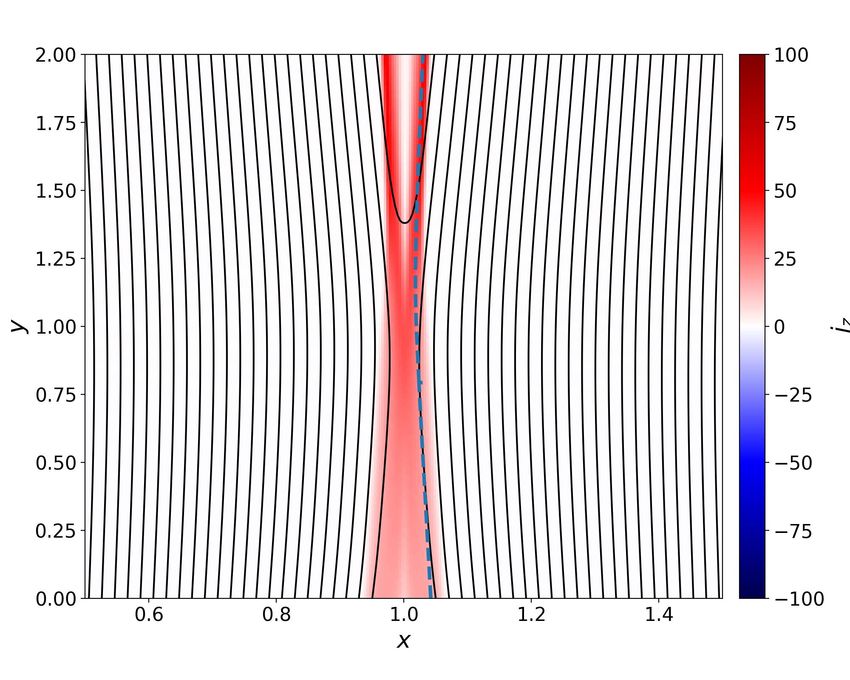
Fast Magnetic Reconnection induced by Resistivity Gradients in 2D Magnetohydrodynamics                                                                             5

                                                                                     Reconnection rate
ing the out-of-plane electric field Ez,xline = ηxline Jz,xline right     (a)                                            (b) 1                                5.0
                                                                                                                                          T1
at the x-line, and they are normalized as R ≡ Ez,xline /(B0VA ),         0.05                                                         η        T5
where B0 is the asymptotic value of the magnetic field at                                     T1
                                                                                                                                                    T6
the upstream region, and VA = B0 /(µρ)1/2 is the Alfvén                  0.03
                                                                                                      T5                      0                              η
speed calculated using this upstream magnetic field and den-                                               T6
sity. The evolution of reconnection rates for different lη are                                                                                               4.2
                                                                         0.01                                              -1
shown in figure 3(a). A uniform resistivity η = 1 × 10⁻³                         0       1   2    3        4    5                 0       1              2
                                                                                             time                                         y
case (U1) is also plotted for comparison. The reconnec-                  (c)                                            (d)
tion rates decrease as lη increases, and it can be explained                                                                  2                              10
                                                                                                        T1          5.0
                                                                                     η
by the following simple analysis; since the normalized rate              0.04                          T5
R = ηxline Jz,xline /(B0VA ) and we know R ' δ /L0 from the                                            T6
                                                                                                                    η     y 1                                0
Sweet-Parker scaling? , where δ and L0 is the half-thickness              0.0
and the length of the “upper” diffusion region (i.e., y > yxline ),
respectively. On the other hand, our simulation demonstrates             -0.04                                      4.2       0                              -10
                                                                                                                                  0       1              2
that L0 ' 2lη and ηxline ' ηbottom . And, we can approximate                     0             1
                                                                                               y
                                                                                                                2
                                                                                                                                          x
Jz,xline ' B0 /(µδ ) in the small diffusion region aspect ratio
(δ /L0 ) limit. Combining all these relations, one can derive the
scaling of the reconnection rate to be                                 FIG. 4. (Run T 1, T 5 and T 6) (a) Reconnection rates with the same
                                                                       resistivity gradient (determined by η1 = 8 × 10⁻⁴ and lη = 0.05) but
                                                                       with a different background resistivity η2 from low to high in Runs
                      r               r
                           ηxline         ηbottom                      T 1 (blue), T 5 (orange), and T 6 (green). (b) The outflow speed vy cut
                 R'               '               .            (10)    at x = 1 at the nonlinear state. (c) The normal magnetic field Bx cut
                          µVA 2lη         µVA 2lη
                                                                       at x = 1 at the nonlinear state. In panels (b) and (c), the resistivity
The reconnection rate is thus determined by both the resistiv-         η of run T 6 is shown as the red line. (d) The current density Jz of
ity gradient length and the resistivity value right at the x-line,     run T 6 at the nonlinear state. While the flux function is slightly bent
                                                                       inside the diffusion region, the rather thick current sheet extend to
which is close to ηbottom in these runs. Figure 3(b) shows the
                                                                       the outflow boundaries.
reconnection rates, averaged after reaching the peak, versus
the resistivity gradient scale length lη in a log-log scale plot.
The simulation results are shown as blue dots and the predic-
                                                                       not increase with a higher background η, then vy Bx should be
tion from equation (10) is plotted as the orange line. R ∝ lη−0.3
                                                                       smaller; this is consistent with the significant drop of Bx and
is also plotted (green line) for comparison, and one can see
                                                                       vy observed in Fig. 4(b) and (c).
that the measured reconnection rates compare better with lη−0.3
                                                                           In addition, the current sheet tends to extend to the out-
scaling, instead of lη−0.5 . This could be caused by the fact that
                                                                       flow boundary if the entire reconnection layer is immersed
the locations of the x-lines are not exactly at the edge where
                                                                       within the non-ideal region with a finite non-ideal electric
resistivity starts to decrease (see Fig. 2). There is also about
                                                                       field ηJz . To illustrate the underlying reason, we will use
a factor of two difference that is not captured by this simple
                                                                       the notations in Figure 5. The inflow and outflow quan-
scaling, but Eq. (10) does qualitatively explain the decreasing
                                                                       tities are evaluated at point i and o, respectively. Point h
trend.
                                                                       is at the middle between the x-line and point o. L0 and δ
   In the following, we also investigate the effect of back-
                                                                       are the half-length and the half-width of the diffusion re-
ground resistivity, that is parametrized by η2 of the hyper-
                                                                       gion. Near the inflow region the out-of-plane electric field at
bolic tangent profile; we increase η2 while keeping the same
                                                                       point i matches the value at the x-line, Ez,i = vx,i By,i ' Ez,xline .
η1 and lη . While the solutions from the averaged-equations
                                                                       At point o, we have Ez,o = vy,o Bx,o + ηJz,o from Ohm’s law
(Appendix A) suggest the increase of reconnection rate, our
simulations show an opposite trend. This is demonstrated by            (Eq. (11)). Using the Maxwell-Faraday’s law ∇ × ~E = −∂t ~B
the Runs in Fig. 4(a) where η1 = 8 × 10⁻⁴ , but Run T 1 has            and the flux conservation vy,o Bx,o ' vx,i By,i , we can estimate
η2 = 2 × 10⁻⁴ , Run T 5 has η2 = 12 × 10−4 , and Run T 6 has           the time derivative of the reconnected field at point h to be
η2 = 42 × 10−4 . The reconnection rates decrease as the back-          ∂t Bx,h ' −∂y Ez ' −(Ez,o − Ez,xline )/L0 ' −(vy,o Bx,o + ηJz,o −
ground resistivity increases.                                          vx,i By,i )/L0 = −ηJz,o /L0 . Therefore, the time derivative of the
   Similar to the thickness of the reconnection diffusion re-          reconnected field at point h is negative (∂t Bx,h < 0) if the cur-
gion, the shock thickness also increases with the background           rent density at point o is finite (Jz,o > 0); a situation that oc-
resistivity. This could introduce a finite current density Jz          curs when there is no clear separation between the pair of slow
within the entire outflow exhaust, as seen in Fig. 4(d). Ac-           shocks at the outflow region. The reconnected magnetic field
cording to Ohm’s law                                                   Bx,h at point h thus tends to decrease with time and the current
                                                                       layer will extend to the boundary, reducing the opening geom-
                         Ez = vy Bx + ηJz                      (11)    etry as seen in Fig. 4(d). Note that this mechanism is different
                                                                       from Kulsrud’s idea discussed in section III. In short, the wide
since Ez along the outflow symmetry line should be uniform in          coverage of the non-ideal region (i.e., the thickening of the
the steady state. If the current density Jz remains significant at     shock transition region) due to a large background resistivity
the outflow region and the reconnection electric field Ez does         causes excessive resistive-diffusion, resulting in an extended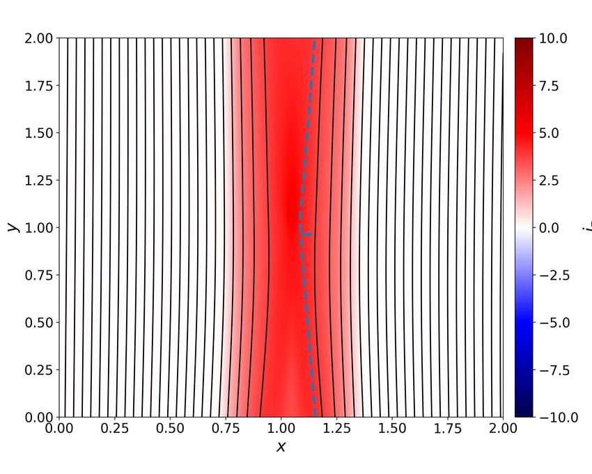
Fast Magnetic Reconnection induced by Resistivity Gradients in 2D Magnetohydrodynamics                                                      6

                                                                           TABLE II. Simulation parameters with a resistivity of exponential
                                                                           profile.
                                                                              Run ηxline = η1 + η2 ηbackground = η2         lη     β
                                                                              E1      5 × 10⁻⁴        1 × 10⁻⁴             0.05   0.1
                                                                              E2      1 × 10⁻³        1 × 10⁻⁴             0.05   0.1
                                                                              E3      1 × 10⁻²        1 × 10⁻⁴             0.05   0.1
                                            L'                                E4      5 × 10⁻²        1 × 10⁻⁴             0.05   0.1
                                                                              E5          1           1 × 10⁻⁴             0.05   0.1

                                                                              From Fig. 6(a), it is clear that, with a fixed resistivity gra-
                                        δ                                  dient scale lη = 0.05, a larger ηxline results in a higher re-
                                                                           connection rate. Panel (b) shows the current density of Run
                                                                           E1, which has a well-localized diffusion region, and the open
                                                                           outflow exhausts are bounded by the sharp transitions of slow
                                                                           shocks. The reconnection rate of this case (' 0.04) is the low-
FIG. 5. The orange rectangle represents the diffusion region. The          est in panel (a) because it has the lowest ηxline = 5 × 10⁻⁴ .
diffusion region length (L0 ) is determined by the imposed resistivity     Run E2 has a higher resistivity ηxline = 1 × 10⁻³ . Its rate is
gradient scale (lη ). The yellow region illustrates the thickness of       shown in red in Fig. (6)(a), which is very close to the rate
downstream slow shock transitions. Point o locates at the end of the       measured in hyperbolic tangent resistivity simulation that has
diffusion region. Point i is at the inflow edge of the diffusion region.   the same η1 + η2 and lη (Run T 1, recall that the x-line devel-
Point h is halfway between the x-line and point o. The thickening          ops close to the high-η end, thus ηxline ' ηbottom = η1 + η2 =
of the shock transition regions due to a large background resistivity
                                                                           1 × 10⁻³ in this run). This is consistent with our expectation
widens the coverage of the non-ideal region, immersing point o with
a finite ηJz .
                                                                           that the resistivity gradient scale and strength right at the x-
                                                                           line determined the rate (if the background resistivity is low
                                                                           enough).
current sheets despite the imposed sharp resistivity gradient.                The most surprising case is Run E5 that has an extremely
   Finally, we also performed simulations (not shown) with a               strong ηxline = 1.0, that is 2000 times larger than that in Run
hyperbolic tangent resistivity profile that varies along a direc-          E1 (Fig. 6(b)). In this case, the current sheet broadens and
tion at a 45◦ angle from the outflow (y-) direction and found              the dramatic drop of the current density right at the x-line is
that Petschek-type reconnection can still be realized. This fur-           a pronounced feature, as shown in Fig. 6(c). Consequently,
ther suggests that the resistivity gradient projected in the out-          the reconnection rate ER = ηxline Jz,xline remains on the order
flow direction is sufficient in facilitating open outflow geom-            of the typical fast rate 0.1? , as shown in Fig. 6(a). This nu-
etry.                                                                      merical experiment demonstrates that the reconnection rate is
                                                                           bounded by physics outside of the diffusion region, presum-
                                                                           ably by the force-balance in the upstream region? . No matter
B.   With a spatially localized η at the x-line                            how strong and localized the resistivity is, the diffusion region
                                                                           is forced to adjust itself to accommodate this maximum plau-
   In this sub-section, we study how the system responds to                sible rate ' 0.2. The slight increase of the rate at E5 near the
an extremely large resistivity spatially localized around the              end comes from the numerical effects at the boundary, which
x-line. For the same reason discussed before, Petschek-type                we will leave for future investigation.
reconnection will be realized because of the presence of resis-               Along this line of discussion, it is also interesting to com-
tivity gradient along the outflow direction. Special attention             pare the maximum reconnection rate predicted by Petschek?
is dedicated here to find the maximum plausible reconnection
                                                                                                                  π
rate potentially applicable to all reconnection systems. To do                                    RPetschek '          ,                 (13)
so, we adopt the following η-profile that exponentially decays                                                  8 ln S
out of the center of the simulation domain (i.e, the x-line).              where S = LVA /η is the Lundquist number, L = 1 is system
                                                                           size, VA is the Alfv́en speed and η is the resistivity. For Run
                                                                           E5 the relevant η is the value near the x-line, ηxline = 1,

                                    r
                   ηexp = η1 exp −      + η2 ,                     (12)    because in Petschek’s derivation η is introduced by match-
                                   lη
                                                                           ing the reconnection electric field at the x-line to the value
where the distance to the center is parameterized by the radius            immediately upstream of the diffusion region; i.e., Ez,xline =
r ≡ [(x − 1)2 + (y − 1)2 ]1/2 . The peak value of the resistivity          ηxline Jz,xline ' vx,i By,i (the same notations used in the discus-
is ηxline = η1 + η2 at the center (x, y) = (1, 1) and the lowest           sion of Fig. 5). Thus, the reconnection rate is predicted to ap-
value is η2 in the background. Figure 6(a) shows the recon-                proach infinity in Petscheck’s model; i.e., 1/ln(1 × 1/1) → ∞
nection rates of different ηxline = η1 + η2 from 5 × 10⁻⁴ to 1.            in Eq. (13). However, the reconnection rate is still on the order
The parameters of the simulations are summarized in table II.              of the typical fast rate value 0.1. This discrepancy likely also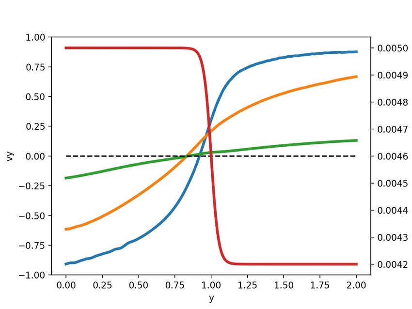
Fast Magnetic Reconnection induced by Resistivity Gradients in 2D Magnetohydrodynamics                                                            7

        (a)                                         (b)                                       (c)
                   Reconnection rate                      2                                100 2                                        100
       0.25
       0.20                    E5
       0.15                       E4
                                                     y1                                    0   y1                                       0
       0.10                    E3
       0.05                  E2
                                           E1
       0.00                                                                                -100                                         -100
              0    1     2       3     4        5             0        1               2            0              1                2
                             time                                      x                                           x

FIG. 6. Panel (a) shows the scaling of reconnection rates in simulations with a spatially localized resistivity at the x-line, including Runs E1
(purple), E2 (red), E3 (green), E4 (orange), and E5 (blue). Panels (b) and (c) show the current density and flux function of Run E1 and Run
E5, respectively, at late time. Note that the current density drops significantly at the x-line for an extremely strong resistivity in panel (c), so
that ηJz remains bounded.

results from the lack of a self-consistent consideration of the             cessible than collisionless plasma in compact devices, and we
force-balance upstream of the diffusion region, that applies to             know how to realize a stable single x-line fast reconnection.
all reconnection systems? , either collisional or colliionless.                In natural plasmas, a resistivity gradient can arise at the
                                                                            sharp transition layer of temperature and density, or at the in-
                                                                            terface between different ion species? ? , such as the solar tran-
V.   SUMMARY AND DISCUSSION                                                 sition region? or the photosphere-chromosphere interface? .
                                                                            The resistivity gradient scale at the interface between the pho-
   In summary, we find that steady Petschek-type fast mag-                  tosphere and chromosphere is estimated as 100 km? , which
netic reconnection can be generated as long as there is an                  is smaller than (or, at least, not larger than) the size of flux
η-gradient along the reconnection outflow direction in MHD                  tubes observed? (≈200-300 km, which will be the system size
simulations. This finding supports the idea of Kulsrud? that                of our simulations). This suggests that our result could be
suggested a resistivity gradient can provide additional supply              relevant to reconnection phenomena occurring in the lower
of the normal magnetic fields within the diffusion region, bal-             solar atmosphere. In particular, our work predicts that solar
ancing the loss by the outflow convection. In simulations with              spicules? ? , if driven by reconnection, may tend to develop at
a resistivity that has a simple hyperbolic tangent profile, the             the altitude of a sharp resistivity gradient .
opening exhaust on one side leads to the opening on the other                  On a separate issue, although resistive-MHD is often
side because the electric field is uniform in a 2D steady-state.            deemed inadequate to address the physics at a diffusion-region
The diffusion region self-adjusts its half-length to fit the re-            scale, it nevertheless allows us to test out the maximum plau-
sistivity gradient length. Therefore, increasing the resistivity            sible reconnection rate in a clean fashion. Specifically, we
gradient length will decrease the reconnection rate.                        can control the strength and localization of resistivity, which
   The solutions of the averaged-equations (Appendix A) pro-                simply cannot be done in fully kinetic simulations; i.e., fully
posed in Refs. ? ? show reasonable agreement with the                       kinetic simulations generate dissipation and diffusion self-
hyperbolic tangent resistivity simulations when the resistivity             consistently? . We found that the reconnection rates are well-
gradient is large and the resistivity background is small. The              bounded by value ' 0.2, no matter how strong the localized
solutions do not agree well with our simulations when there                 resistivity is. The existence of this upper bound can be ex-
is a large background resistivity or a small resistivity gradi-             plained by the upstream force-balance in the MHD region? .
ent, and we provide an explanation to address the effect of                 This fact has a significant implication, suggesting that a strong
large background resistivity. Besides, the reconnection rates               anomalous resistivity will not further increase much the typ-
predicted by the averaged-equations are not bounded in the                  ical fast rate of order 0.1 reported in 2D laminar kinetic
large background η limit. It is likely due to the lack of con-              simulations? ? . Notably, the reconnection rates observed by
sideration on the upstream force-balance, which is critical in              NASA’s Magnetospheric Multiscale (MMS) mission? ? ? ? ?
limiting the reconnection rate? .                                           are consistently bounded by the maximum plausible value 0.2
   This work demonstrates that anti-parallel magnetic fields                demonstrated here.
that thread these two regions will prefer to reconnect at this                 In conclusion, this work shows that a resistivity gra-
interface, where the energy release is most efficient. The fact             dient can efficiently induce a spatially localized diffusion
that we can induce fast reconnection in collisional plasmas us-             region and fast reconnection in collisional plasmas. We
ing resistivity gradient, and confine the x-line within the tran-           further expect that if the local reconnection electric field
sition region, may be handy for the design of reconnection-                 excesses the Dreicer runaway value, the diffusion region
based thrusters? ; i.e., a collisional plasma might be more ac-             plasma transitions to the collisionless regime? ? , and kinetic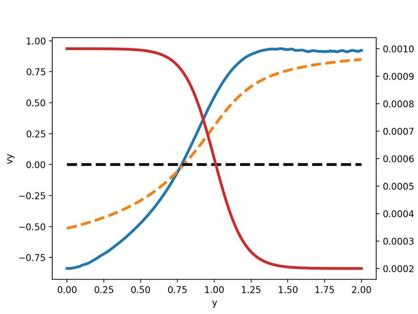
Fast Magnetic Reconnection induced by Resistivity Gradients in 2D Magnetohydrodynamics                                                  8

physics? ? ? ? ? ? ? ? ? can take over to continue fast reconnec-      In the following, magnetic field B is normalized to the up-
tion.                                                               stream magnetic field (B0 ), velocity to the upstream Alfv́en
                                                                                √
                                                                    speed (B0 / µ0 ρ0 ), density to the density at a(y) (ρa ), pres-
                                                                    sure to the upstream magnetic pressure (B20 /2µ0 ), µ0 = 1, and
ACKNOWLEDGMENTS                                                     length to the system size (L). Therefore, Bya = 1, ρa = 1,
                                                                    pa = β /2 are assumed, and we drop off the angle brackets for
  We gratefully acknowledge helpful discussions with                convenience. The averaged-equations become
Michael Hesse, Judit Pérez-Coll, Terry Forbes, Jongsoo Yoo,
Jim Klimchuk, and Chengcai Shen. Contributions from S.L.,            aρvy = MA (y − ysp )                                    (A6)
Y.L. and X.L. are based upon work funded by the National              d
Science Foundation Grant No. PHY-1902867 through the                    (ρv2y a) = Bx                                        (A7)
                                                                     dy
NSF/DOE Partnership in Basic Plasma Science and Engineer-            "                  #
                                                                       ρv2y γ(1 + β )

ing and NASA MMS 80NSSC18K0289.                                                                      γβ
                                                                           +              avy =            + 1 MA (y − ysp ) (A8)
                                                                        2      2(γ − 1)           (γ − 1)2
                                                                                                          η(y)
DATA AVAILABILITY                                                    Ea = MA = −vxa Bya = Bx vy +              ,                    (A9)
                                                                                                           a
   Raw data were generated at the NERSC Advanced Super-             where ysp is the position of the flow stagnation point and
computing large scale facility. Derived data supporting the         MA is the inflow Alfv́en Mach number. Baty et. al.? fur-
findings of this study are available from the corresponding au-     ther combines these equations into a single ODE by plugging
thor upon reasonable request                                        Eqs. (A6), (A7) and (A8) into Eq.(A9) ,
                                                                                          dvy       1    ρη(y)
                                                                             (y − ysp )       + vy = − 2             ,             (A10)
Appendix A: Averaged MHD Equations                                                        dy        vy MA (y − ysp )

   To get a more quantitative comparison to our simulation          where
results, here we introduce the averaged MHD equations de-                                            5(1 + β )
rived by Refs. ? ? . Physical quantities inside the diffusion                                 ρ=                                   (A11)
                                                                                                   5β + 4 − 2v2y
region, in the steady-state, are averaged across the reconnec-
tion layer (illustrated in Fig. 7) to reduce the full MHD partial   is the averaged density of plasma inside the diffusion region
differential equations (PDEs) into a much simpler system of         and γ = 5/3 is used.
ordinary differential equations (ODEs), that depends only on           Given an η(y) profile, MA and ysp can be solved by expand-
coordinate y. For a given resistivity profile, one can then solve   ing vy and η with respect to ysp
for the averaged outflow speed, current sheet width, and av-
eraged normal (reconnected) magnetic field. In this work, we          vy = v1 (y − ysp ) + v2 (y − ysp )2 + v3 (y − ysp )3 + ...   (A12)
apply this theory using the hyperbolic tangent resistivity pro-                                                    2
                                                                       η = η0 + η1 (y − ysp ) + η2 (y − ysp ) + ...,               (A13)
files (Eq. (6)) and compare the solutions with our numerical
simulations in Figures 1, 2, and 4.                                 By plugging these expansions into equation (A10) and solving
   The averaged continuity equation, momentum equation, en-         for the coefficients, one can get
ergy equation, and Ohm’s law are derived to be
                                                                                                       (5β + 4)MA2
                                                                                                v1 =                               (A14)
    d                                                                                                  5(1 + β )η0
      (ahρihvy i) = −ρa vxa ,                               (A1)
   dy                                                                                                η1 (5β + 4)MA2
                                                                                            v2 = −                                 (A15)
    d                    dhpi                                                                         η02 5(1 + β )
      (hρihvy i2 a) = −a       + Bya hBx i,                 (A2)
   dy                     dy
          hρihvy i2 γhpi

    d                                          γ pa                         (5β + 4)MA2
                    +         ahvy i = −            + B2ya vxa ,    v3 =                 −2(4 + 5β )MA4 + 5(1 + β )(η12 − η0 η2 )

   dy         2       γ −1                    γ −1                                   2 3
                                                                           25(1 + β ) η0
                                                            (A3)                                                           (A16)
                     ηBya
   Ea = hvy ihBx i +      ,                                 (A4)            (4 + 5β )MA2
                       a                                            v4 =                    [25(1 + β )2 (−η13 + 2η0 η1 η2 − η02 η3 )
                                                                           125(1 + β )3 η04
where a(y) is the half-width of the current sheet, physical
quantities with subscript “a” indicate their values at x = a(y),    + (4 + 5β )(34 + 35β )η1 MA4 ]                                 (A17)
and the averaged quantities are defined by averaging over x
from 0 to a(y),                                                       The condition for convergence is obtained by requiring the
                                  Z a                               coefficients of higher order terms to vanish,
                              1
                   hAi(y) ≡             A(x, y)dx.          (A5)                                 lim vn = 0.
                              a    0                                                             n→∞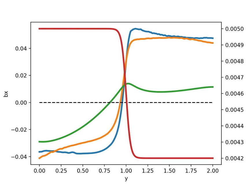
Fast Magnetic Reconnection induced by Resistivity Gradients in 2D Magnetohydrodynamics                                                                     9

                                                                                  B

FIG. 7. Petschek-type reconnection configuration. The inflow is in the x-direction and the outflow is in the y-direction. Solid arrows indicate
magnetic fields. Dashed lines bound the current sheet, inside which are the diffusion region, the transition region, and the downstream region
of standing slow shocks.

We take vn = 0 and vn+1 = 0 for n = 3 since v1 and v2 are                      Using the un-averaged Ohm’s law,
the lowest order terms needed to reproduce the bi-directional
outflows. Baty et. al.? solved MA and ysp using different val-
ues of n and showed that their numerical values do not change
much if n ≥ 3, as shown in table I and II in their paper. After
solving numerical values of MA and ysp by setting Eqs. (A16)                          Ez (a, y) = vy (a, y)Bx (a, y) + η(a, y)Jz (a, y),             (A20)
and (A17) to zeros, the averaged outflow speed vy can be ob-
tained numerically by solving Eq. (A10). Note that the av-
eraged equation Eq. (A4) should capture the physics of Kul-
srud’s mechanism. To see this, we take the y-derivative of the
z-component of the averaged Ohm’s law, which gives
        Z a                                                                    we have
   ∂y          Ez (x, y)dx =
        Z0 a                               Z a
   ∂y          vy (x, y)Bx (x, y)dx + ∂y         η(x, y)Jz (x, y)dx.   (A18)
         0                                  0                                      Z a
Applying the fundamental theorem of calculus, we get                                      ∂y Ez (x, y)dx =
     Z a                                                                           Z0 a                                  Z a
                           da                                                             ∂y (vy (x, y)Bx (x, y)) dx +         ∂y (η(x, y)Jz (x, y)) dx,
         ∂y Ez (x, y)dx + Ez (a, y) =                                                 0                                   0
      0                    dy
     Z a                                                                                                                                   (A21)
                                      da
         ∂y (vy (x, y)Bx (x, y)) dx + vy (a, y)Bx (a, y)+                      This is the induction equation (7) averaged over x from 0 to
      0                               dy
     Z a                                                                       a(y), which was used to derive Eq. (8). Figure 1 has shown
                                     da                                        the prediction of a(y) in panel (a), vy (y) in panel (b) and Bx (y)
         ∂y (η(x, y)Jz (x, y)) dx + η(a, y)Jz (a, y).     (A19)
      0                              dy                                        in panel (c) for Run T1 . The agreement is reasonable.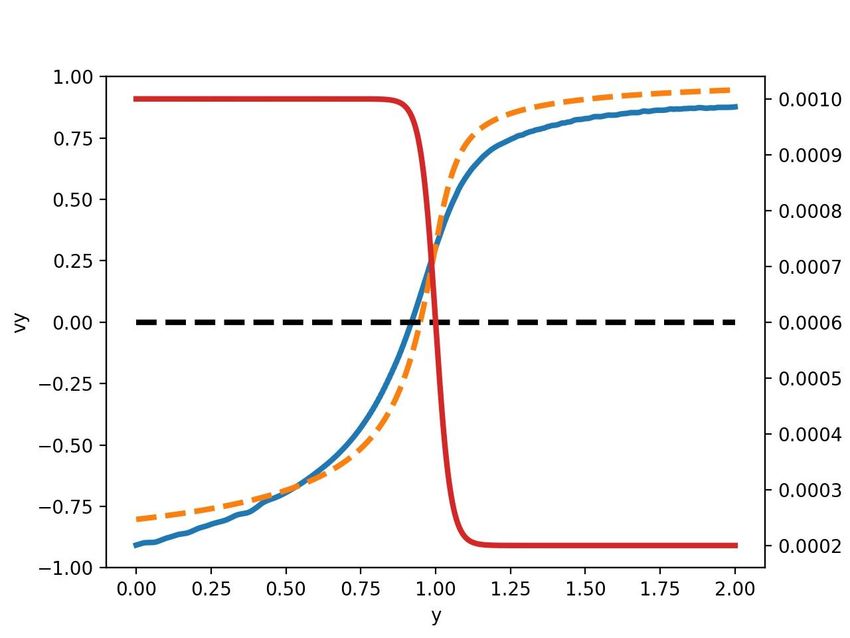
You can also read