Transportation Research Part C
←
→
Page content transcription
If your browser does not render page correctly, please read the page content below
Transportation Research Part C 129 (2021) 103250
Contents lists available at ScienceDirect
Transportation Research Part C
journal homepage: www.elsevier.com/locate/trc
A hybrid Delphi-AHP multi-criteria analysis of Moving Block and
Virtual Coupling railway signalling
Joelle Aoun a, *, Egidio Quaglietta a, Rob M.P. Goverde a, Martin Scheidt b,
Marcelo Blumenfeld c, Anson Jack c, Bill Redfern d
a
Delft University of Technology, Department of Transport and Planning, Stevinweg 1, 2628 CN Delft, The Netherlands
b
TU Braunschweig, Institute of railway systems engineering and traffic safety, Pockelstrasse 3, 38106 Braunschweig, Germany
c
University of Birmingham, College of Engineering and Physical Sciences, Edgbaston, Birmingham, B15 2TT Birmingham, United Kingdom
d
PARK Signalling ltd., Houldsworth Mill, Houldsworth St., Reddish, Stockport SK5 6DA, United Kingdom
A R T I C L E I N F O A B S T R A C T
Keywords: The railway industry needs to investigate overall impacts of next generation signalling systems
Railway operations such as Moving Block (MB) and Virtual Coupling (VC) to identify development strategies to face
Moving block signalling the forecasted railway demand growth. To this aim an innovative multi-criteria analysis (MCA)
Virtual coupling
framework is introduced to analyse and compare VC and MB in terms of relevant criteria
Multi-criteria analysis
Delphi
including quantitative (e.g. costs, capacity, stability, energy) and qualitative ones (e.g. safety,
AHP regulatory approval). We use a hybrid Delphi-Analytic Hierarchic Process (AHP) technique to
objectively select, combine and weight the different criteria to more reliable MCA outcomes. The
analysis has been performed for different rail market segments including high-speed, mainline,
regional, urban and freight corridors. The results show that there is a highly different techno
logical maturity level between MB and VC given the larger number of vital issues not yet solved
for VC. The MCA also indicates that VC could outperform MB for all market segments if it reaches
a comparable maturity and safety level. The provided analysis can effectively support the railway
industry in strategic investment planning of VC.
1. Introduction
The railway industry urges to increase transport capacity of existing networks to address the forecasted growth in the railway
demand. Research is hence focusing on reducing the safe train separation distances of traditional fixed-block railway operations by
introducing train-centric signalling concepts which migrate more and more trackside vital equipment to train-borne equipment using
radio communication.
Moving Block (MB) signalling (Theeg and Vlasenko, 2009) envisages that the train is equipped with devices for continuous train
positioning, Train Integrity Monitoring to guarantee a safe train-rear position, dynamic braking curve supervision, and wireless
communication for sending position reports and receiving movement authorities from radio block centres. In this setup, traditional
block sections can be removed together with corresponding line-side equipment so that train separation can be reduced to an absolute
* Corresponding author.
E-mail addresses: J.Aoun@tudelft.nl (J. Aoun), E.Quaglietta@tudelft.nl (E. Quaglietta), R.M.P.Goverde@tudelft.nl (R.M.P. Goverde), M.
Scheidt@tu-bs.de (M. Scheidt), M.Blumenfeld@bham.ac.uk (M. Blumenfeld), A.C.R.Jack@bham.ac.uk (A. Jack), Bill.Redfern@park-signalling.co.
uk (B. Redfern).
https://doi.org/10.1016/j.trc.2021.103250
Received 29 January 2021; Received in revised form 6 May 2021; Accepted 29 May 2021
Available online 10 June 2021
0968-090X/© 2021 The Authors. Published by Elsevier Ltd. This is an open access article under the CC BY license
(http://creativecommons.org/licenses/by/4.0/).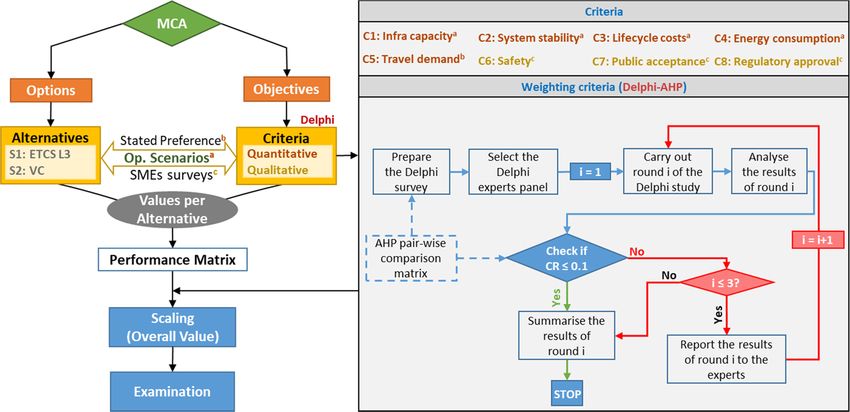
J. Aoun et al. Transportation Research Part C 129 (2021) 103250
braking distance (i.e. the distance needed to brake to a standstill). MB signalling for conventional railways finds an implementation in
the European standard: European Train Control System (ETCS) Level 3. Therefore, new railway signalling and control technology are
being developed that can significantly increase railway capacity and overall performance.
The concept of Virtual Coupling (VC) advances MB operations by reducing train separation to less than an absolute braking distance
using Vehicle-to-Vehicle communication. By mutually exchanging dynamic information (e.g. position, speed, acceleration), trains can
be separated by a relative braking distance (i.e. the safe distance of a train behind the rear of the predecessor taking into account the
braking characteristics of the train ahead) even when this predecessor executes an emergency braking, while ensuring a safety margin.
This is particularly beneficial when trains move synchronously together in a virtually coupled state within a platoon. Those platoons
could hence be treated as a single train at junctions thereby greatly increasing capacity at network bottlenecks.
Several critical safety issues are however still unaddressed for the VC concept. Crucial is for instance the risk of splitting platoons at
diverging junctions where a switch must be locked before a train is at the absolute braking distance so that it can still brake in case of
failure. The railway industry has an urgent need to investigate limitations and advantages of VC over simple MB before proceeding
with potential investment decisions. An overall analysis is hence necessary to identify effects that VC could have in terms of technical,
technological, societal and environmental criteria. This paper contributes to address this necessity by performing an extensive multi-
criteria impact analysis of VC in comparison with ETCS Level 3 MB and traditional fixed-block signalling systems for different railway
market segments. The analysis has been made in the context of the European project MOVINGRAIL (2018) funded by the Shift2Rail
programme (Shift2Rail, 2020). An innovative multi-criteria analysis framework is introduced to evaluate impacts of VC on lifecycle
costs, infrastructure capacity, energy, service stability and travel demand as well as on qualitative criteria such as regulatory approval,
public acceptance and safety.
The main contributions of this paper are: i) the application for the first time in railway literature of a hybrid Delphi-Analytic
Hierarchy Process (Delphi-AHP) approach to assess impacts of railway signalling innovations; ii) the definition of a multi-criteria
framework encompassing multiple interdisciplinary methods for evaluating technical, technological, operational and societal/regu
latory criteria; iii) the definitions of new indexes that –to the best of our knowledge– were not identified in previous published works,
and iv) for the first time a general evaluation of VC effects is provided which can provide the railway industry with more elements to
support strategic investment and development plans.
In Section 2 of this paper a literature review on train-centric signalling systems and multi-criteria methods is provided. The Multi-
Criteria Analysis (MCA) methodological framework introduced in this study is described in Section 3. Section 4 presents operational
scenarios and the methods used to compute each criterion. Section 5 displays case studies considered for the different railway market
segments and reports the final results of the MCA. Conclusions and recommendations are eventually provided in Section 6.
2. Literature review
2.1. Train-centric signalling systems
In traditional fixed-block signalling systems, trains are separated by one or more block sections with movement authorities pro
vided by line-side (multi-aspect) signals or radio-based cab signalling like ETCS Level 2 (Theeg and Vlasenko, 2009). MB signalling
Fig. 1. Schematic architecture of train-centric signalling systems: Moving Block (a) and Virtual Coupling (b).
2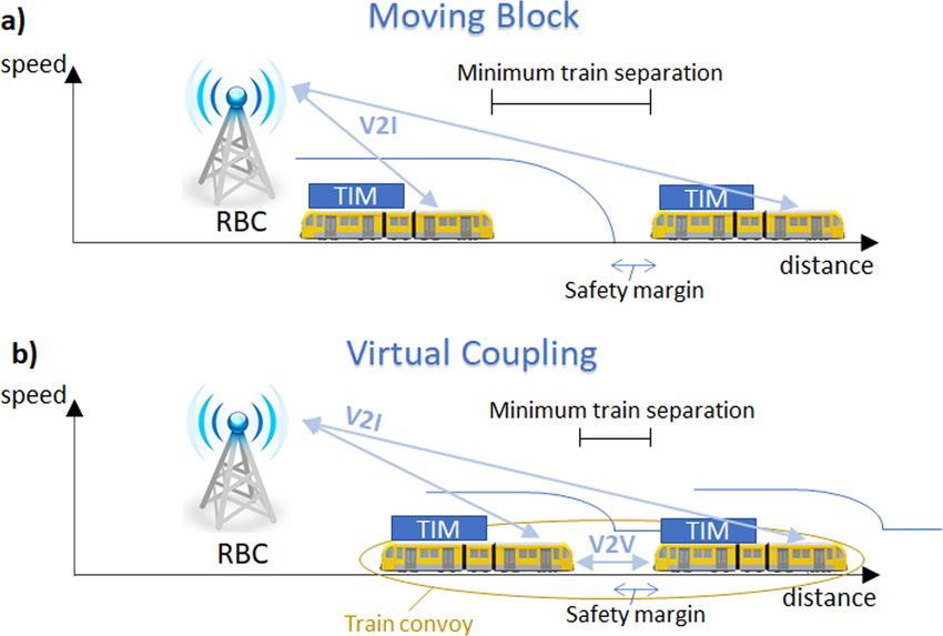
J. Aoun et al. Transportation Research Part C 129 (2021) 103250
reduces train separation to an absolute braking distance by removing track block sectioning and migrating vital track-clear detection
equipment to on-board integrity monitoring. The ETCS Level 3 standard gives requirements for MB railway operations (Fig. 1a). A
track-side Radio Block Centre (RBC) sends Movement Authorities (MAs) to the trains indicating the maximum distance that the train
can safely run based on regularly updated train position reports. The on-board European Vital Computer (EVC) ensures that the MAs
are respected by computing and supervising dynamic speed profiles including continuous braking curves. Verification of train integrity
is performed by an on-board device called Train Integrity Monitoring (TIM) which is still an open challenge for trains with variable
composition such as freight trains. The British and Dutch railway infrastructure managers propose a hybrid version of ETCS Level 3
which leaves in place track-clear detection devices to monitor train integrity for trains unequipped with TIM (Furness et al., 2017).
Legrand et al. (2016) propose instead an integrity monitoring technology that can meet required safety standards by combining Global
Navigation Satellite Systems (GNSS) with Inertial Navigation Systems (INS). Biagi et al. (2017) show how missed train integrity and/or
position reporting due to communication break-up in ETCS Level 3 can drastically reduce network capacity.
MB operations such as made possible by ETCS L3 have been upgraded recently by the concept of VC which postulates the possibility
that trains could just be separated by a relative braking distance plus a safety margin, so to increase even further infrastructure capacity
utilisation. As illustrated in Fig. 1b, VC enriches the basic MB architecture with a Vehicle-to-Vehicle (V2V) communication layer to
allow trains to exchange dynamic information (e.g. position, speed and acceleration), which is needed to supervise relative braking and
keep a safe separation. The virtually coupled trains form a train convoy that is treated as a single train at junctions, so that switches
remain locked until the entire convoy has passed. VC also enables the formation of platoons where trains can move synchronously with
each other at close distance, thereby increasing capacity. Due to the very short train separation, automatic train operation becomes
essential for VC given that human driving reaction times would no longer be safe in this setup. Several challenges still need to be
addressed for VC. One main issue regards diverging junctions where a separation shorter than a full braking distance is not yet possible
as it could lead to unsafe train movements in case of longer switch setup times or switch locking failures. Another issue relates to the
V2V communication architecture that requires high levels of reliability and low latency for the exchange of safety–critical information
among trains. European projects such as X2Rail-3 (2018) and MOVINGRAIL (2018) have been investigating safe operational princi
ples, scenarios and reliable communication architectures for the feasibility of VC. Fenner (2016) presented steps and scenarios for
closer running, i.e. VC. Schumann (2017) simulated the ‘Shinkansen’ scenario to increase line capacity on the Tokaido high-speed line
in Japan by following the VC principles. Flammini et al. (2019) proposed a quantitative model to analyse the effects of introducing
Virtual Coupling according to the extension of the current ETCS Level 3 standard, by maintaining the backward compatibility with the
information exchanged between trains and the trackside infrastructure. Felez et al. (2019) developed a preliminary Model Predictive
Control approach for virtually coupled trains using a predecessor-following information structure that minimizes a function of desired
safe relative distance, the speed of the predecessor train and the jerk. Di Meo et al. (2019) studied operational principles and
communication configurations of VC in several stochastic scenarios by using a numerical analysis approach. Quaglietta et al. (2020)
illustrated preliminary capacity benefits of VC over MB for a British mainline case study, by applying a multi-state train following
model. The main question that literature has not clarified yet is whether the trade-off between overall benefits and costs of VC are more
advantageous to the transport industry than MB signalling. This paper tries to address this fundamental research question by
implementing an innovative multi-criteria analysis framework to compare impacts of VC with MB and traditional fixed-block sig
nalling systems.
2.2. Multi-criteria analysis methods
Multi-Criteria Analysis (MCA) is a scientific method to support practitioners in making effective decisions with respect to several
conflicting criteria (Kumru and Kumru, 2014; Miettinen, 2012). An MCA is similar in many aspects to a Cost-Effectiveness Analysis
(CEA) that compares the relative costs and effects of different alternatives, but involving multiple indicators of effectiveness (Pearce
et al., 2006).
The Multi-Criteria Decision Making (MCDM) methods provide decision makers with some tools to solve a complex problem where
different points of view are taken into account (Vincke,1992). The first step for performing a MCA is to correctly identify the main
criteria which need to be assessed to address a specific design/evaluation problem. One of the main approaches applied in literature to
determine critical evaluation criteria is the Delphi method which has been firstly introduced in 1950s (Dalkey and Helmer, 1963;
Linstone, 1978). Delphi consists of combining points of view and opinions from a group of individuals by means of iterative ques
tionnaires with controlled feedback. Four key features are regarded as necessary to define a ‘Delphi’ procedure: anonymity, iteration,
controlled feedback and statistical aggregation of group responses (Rowe and Wright, 1999). The Delphi technique has been exten
sively used in various sectors including forecasting, planning, curriculum development (Thangaratinam and Redman, 2005), health
care (Morgan, 1982) and transportation (Da Cruz et al., 2013). Once the main criteria are identified, several MCDM methods are
available in literature to an objective criteria assessment. The Analytic Network Process (ANP) facilitates feedback and interaction
capabilities among different cited elements within and between groups (Saaty, 2001). The ELimination Et Choix Traduisant la REalité
(ELECTRE) method is used to choose the best actions from a given set of actions. Main applications of the ELECTRE are usually found to
solve three types of problems: choosing, ranking and sorting. The main limitation of this approach is due to the high subjectivity of
calculated ELECTRE thresholds which might lead to unreliable results (Gavade, 2014). The Weighted Sum Method (WSM) is one of the
earliest and simplest techniques that supports single dimensional problems and where overall results are provided in a qualitative form
such as ‘good, better, best’ (Singh and Malik, 2014). The Multi-Attribute Utility Theory (MAUT) is a “rigorous methodology to
incorporate risk preferences and uncertainty into multi criteria decision support methods” (Loken, 2007), but it has the shortcoming of
being data intensive requiring an incredible amount of input at every step of the procedure in order to accurately record the decision
3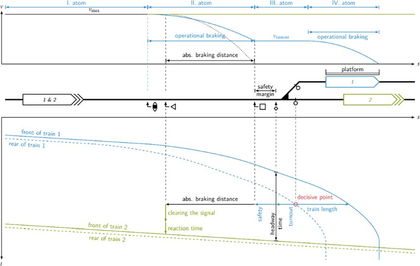
J. Aoun et al. Transportation Research Part C 129 (2021) 103250
maker’s preferences (Velasquez and Hester, 2013). The Technique for Order of Preference by Similarity to Ideal Solution (TOPSIS) was
developed by Hwang and Yoon (1981) and is based on selecting the shortest distance from the positive ideal solution (i.e. best possible
combination of criteria) and the longest distance from the negative ideal solution (i.e. worst criterion values). TOPSIS is an easy
deterministic method which does not consider uncertainty in weightings (Gavade, 2014).
A more objective and comprehensive MCA method is the Analytic Hierarchy Process (AHP) developed by Saaty (1980) which is a
compensatory scoring method that eliminates incomparability between variants built on a utility function of aggregated criteria (Xu
and Yang, 2001). The AHP is considered as a systematic and terse method (Li et al., 2017) applicable to decision-making problems with
complex hierarchies. Applications of the AHP are found in different areas ranging from the socio-economic sector (Kumru and Kumru,
2014) to transportation (Macharis and Bernardini, 2015). Feretti and Degioanni (2017) identified the AHP to be particularly appro
priate to railway management related problems. Barić and Starčević (2015) showed that more than 18% of railway MCA projects make
use of the effective AHP method (e.g. Gerçek et al., 2004; An et al., 2011; Kumru and Kumru, 2014).
Based on the outcomes of this literature review, AHP has been selected in our research as the most appropriate MCA method to
assess the impacts of VC railway signalling which is considered as an innovative and at the same time complex step change for the
railway sector. Specifically, we will be relying on a hybrid Delphi-AHP approach to have a more objective identification of the most
relevant assessment criteria and ensure consistency in the pairwise comparison matrix for criteria weighting, which is required for the
calibration of the AHP technique. This hybrid Delphi-AHP represents a contribution to railway science since it is the first time it is
applied in this specific sector.
3. Methodology
In this section, the MCA framework is introduced where the focus is on the Analytic Hierarchy Process (AHP) and the Delphi
methods. Sections 3.2 and 3.3 are part of existing theories available in the literature review (Section 2), whereas the innovative
framework is built on combinatorial methods, consolidated mathematical techniques, engineering procedures, and extensive Subject
Matter Expert (SME) interviews and workshops to assess each of the criteria defined in Section 1. The elements of this framework are
further detailed in Section 4 where the developed methodologies are applied in Section 5.
3.1. MCA framework
The described MCA framework is illustrated in Fig. 2. The MCA builds on two main elements: alternatives (derived from options)
and criteria (derived from objectives). An alternative is a choice defined between two or more possibilities (i.e. options). A criterion
instead is generated based on the objectives that the decision-maker would like to achieve. For example, the selection of a ‘population’
criterion could be based on the objective of engaging alternatives where the population is greater than a value “x”. The set of alter
natives and criteria is usually specified by a group of decision makers, mainly stakeholders or SMEs. Each alternative possesses its own
values of criteria which can be either quantitative or qualitative depending on the defined objective(s). Criteria for buying a new car
could for example be quantitative such as cost and engine power or qualitative such as user’s comfort and overall look. Assume that an
individual hesitates about the car to buy and there are five alternatives available (Alternative A1 for car 1, A2 for car 2, …, A5 for car
5). The decision-maker needs to choose the suitable car based on a set of criteria (e.g. cost, engine power, durability, comfort, etc.).
Fig. 2. MCA Framework.
4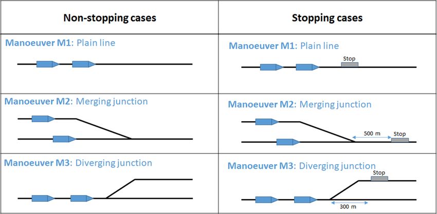
J. Aoun et al. Transportation Research Part C 129 (2021) 103250
Each alternative m possesses its own value of Criteria n (i.e.Xm,n ). For instance, alternative A1 possesses its own value of the first criteria
cost for alternative A1 (i.e. X1,1 ), A2 possesses its own value of cost X2,1 , etc. In the same manner, alternative A1 possesses its own value
of comfort X1,2 , A2 is assigned with X2,2 , etc.
In this paper, the interactions between alternatives and almost all of the quantitative criteria (i.e. infrastructure capacity, system
stability, lifecycle costs and energy consumption) depend on different operational scenarios described in Section 4. Stated preference
surveys are involved to assess travel demand distribution, and stakeholders’ judgement is used for safety, public acceptance and
regulatory approval. After combining the different combinations of criteria values per alternative, a performance matrix is constructed.
Criteria are weighted by means of the hybrid Delphi-AHP method (Section 3.3). Based on the set of expertise required for the survey, a
panel of experts is accordingly selected. Then a round of the Delphi survey is performed and survey results are analysed in terms of
consistency of the AHP pairwise comparison matrix. In case the consistency ratio of the relative criteria assessment is above the
threshold of 0.1, all the respondents providing inconsistent matrices are required to re-do the survey so to give consistent responses (i.
e. Consistency Ratio CR ≤ 0.1). After each round of the AHP pairwise comparison matrix, the survey results are distributed anony
mously to the interviewed panel for further feedback until final consistent results are returned. The Delphi rounds are further discussed
in Section 5.3 and the number of rounds has been limited to three as Walker and Selfe (1996) claim that “repeated rounds may lead to
fatigue by respondents”, and most studies use two or three rounds (Arof, 2015). After the first round of the hybrid Delphi-AHP method,
we further guided the interviewees to provide consistent responses. Particularly, we created a dynamic Excel sheet that automatically
syncs the matrix with the final value of the consistency ratio, so that the interviewees can alter the values of their matrices accordingly
until reaching a CR ≤ 0.1. Then, decision matrices are normalized and weighted to ultimately provide an overall value for each
alternative. In this paper, the examination process consists of enabling cohesion among the different points of view of the involved
SMEs, and evaluating consistency to reach a reasonable consensus matrix by statistically aggregating responses. Finally, results are
evaluated and shared with the respondents. This framework can be also applicable to other fields by just modifying the alternatives and
criteria according to the investigating study.
3.2. The Analytic Hierarchy Process (AHP)
Three main steps are involved in the determination of weights in the AHP technique:
1) Building the hierarchical model
2) Constructing the pairwise comparison judgment matrix
3) Checking consistency.
Step 1: Building the hierarchical model
The hierarchical model consists of three main layers. The top layer represents the overall goal for determining the ranking of
importance. The middle level displays the multiple criteria which influence the goal. Those criteria are used for evaluating the al
ternatives that constitute the bottom level of the hierarchical model (Bhushan and Rai, 2004). In other words, each alternative has its
own values of criteria associated with it. Fig. 3 shows the Analytic Hierarchy Process model where the goal layer is denoted as A, the
middle level consists of n criteria denoted as C1, C2, …, Cn and the bottom level consists of m (signalling) alternatives denoted by S1, S2,
…, Sm.
Step 2: Constructing the pairwise comparison judgement matrix
A judgement matrix evaluates and prioritizes a list of options where the decision-maker provides weighted criteria that are assessed
with respect to each other in a n × n matrix. The judgement matrix for criteria weighing is constructed by pairwise comparing two
elements (Saaty, 2008; Dieter and Schmidt, 2013). The pairwise comparisons are used to determine the relative importance of each
element of one layer to the element of the above layer. In this paper, we consider one level of pairwise comparison which consists of
Fig. 3. Analytic Hierarchy Process model.
5
J. Aoun et al. Transportation Research Part C 129 (2021) 103250
determining the relative importance of each criterion C1, C2, …, Cn with respect to the goal A (see Fig. 3). The other level of assessing
each alternative S1, S2, …, Sm with respect to each criterion C1, C2, …, Cn is out of the scope of this analysis since decision makers
considered railway signalling alternatives equally important with respect to each criterion. The decision-maker has to express his/her
opinion about the value of one single pairwise comparison at a time based on a scale of relative importance that ranges from 1 to 9
where a value of 1 means that the compared criteria are of equal importance. The lower bound of 2 signifies weak or slight importance
whereas a value of 9 refers to absolute or extreme importance. The remaining values are uniformly intermediate ranging from 3
(moderate importance) to 8 (very strong importance). The judgment value of the importance of element i with respect to element j is rij ,
the reciprocal value is 1/rij . For instance, a matrix value of 9 means that the criterion on the row is absolutely more important than the
one on the column, whereas a value of 1/9 means that the criterion on the column is absolutely more important than the one on the
row. The number of comparisons within the level is based on the equation: n(n − 1)/2 where n is the number of comparable elements (i.
e. in this case the number of criteria).
Step 3: Checking consistency
After constructing the pairwise comparison matrix, matrix values Ci,j on row i of criterion i and column j of criterion j are
normalized (as the term Ci,j ) by the sum of the values on all rows of column j where n is the total number of comparable elements:
∑
n
Ci,j
Ci,j = , i, j ∈ {1, ⋯, n} (1)
l=1
Cl,j
Weights Cw,i for a criterion on row i are then computed as the average of the normalized values Ci,j across the total number of
comparable elements n on that row:
∑
n
Ci,j
Cw,i = , i ∈ {1, ⋯, n} (2)
j=1
n
The vector of weights is called priority vector or ‘normalized principle Eigenvector’ (Kumru and Kumru, 2014). An eigenvector is
computed based on the normalized judgement matrix. However, inconsistencies might arise when many pairwise comparisons are
performed (i.e. high number of criteria). For example, if a decision-maker evaluates criterion C1 as more important than criterion C2
and criterion C2 more important than criterion C3, an inconsistency arises if criterion C3 is assessed as more important than criterion C1.
The purpose of matrix consistency is to ensure that the judgement is rational and avoid conflicting results.
Before computing the Consistency Ratio (CR) of the consolidated pairwise comparison matrix, the maximum eigenvalue λmax needs
to be calculated. This eigenvalue is defined as the average of the ratios obtained from the weighted sum on row i and the corresponding
criterion weight Cw,i . Here, the weighted sum is defined as the sum of the relative importance values Ci,j multiplied by the corre
sponding criterion weight Cw,i over the columns j of row i. Hence, λmax is computed as:
∑
n
λi ∑
n
Ci,j Cw,j
λmax = , with λi = . (3)
i=1
n j=1
Cw,i
Note that λmax ≥ n and λmax − n measures the deviation from the judgements from the consistent approximation. A Consistency Index
(CI) is then calculated as:
(λmax − n)
CI = . (4)
n− 1
Finally, the Consistency Ratio (CR) is obtained by dividing CI by the Random Index (RI) associated with the number of comparable
elements n with values as displayed in Table 1 (Saaty, 1980), i.e.,
CI
CR = . (5)
RI
For each criterion, performance values Xm,n obtained for criterion n and signalling alternative m have been normalized (Xm,n ) with
respect to the maximum (for beneficial criteria) or the minimum (for non-beneficial criteria) value over all the signalling alternatives:
• For beneficial criteria:Xm,n = Xm,n /max(Xl,n ).
l
( )/
• For non-beneficial criteria: Xm,n = min Xl,n Xm,n .
l
Finally, the ranking of alternatives is obtained by computing the weighted MCA performance scores Pm (6) defined as the weighted
sum (by the criterion weights Cw,n ) over the total number Nc of criteria n per signalling alternative m, for a given market segment.
Table 1
The RI Values.
No. Elements 1 2 3 4 5 6 7 8 9 …
RI 0 0 0.58 0.90 1.12 1.24 1.32 1.41 1.45 …
6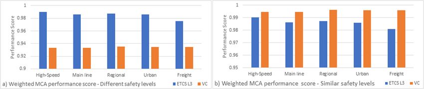
J. Aoun et al.                                                                                        Transportation Research Part C 129 (2021) 103250

                 ∑Nc
         Pm =     n=1
                        X m,n ⋅ Cw,n .                                                                                                           (6)

3.3. A hybrid Delphi-AHP approach

    The hybrid Delphi-AHP technique aims at combining the Delphi technique with the AHP MCDM method described in Sections 2.2
and 3.2. This technique has been traced in many research areas such as project management (Lee and Kim, 2001), logistics (Cheng
et al., 2008), shipping (Lee et al., 2014), forecasting (Mishra et al., 2002) and safety (Chung and Her, 2013). However, to the best of our
knowledge, it has not been used in the railway sector. Arof (2015) showed that usually the number of participants involved in a Delphi
survey is different than those involved in an AHP survey. The number of panellists generally depends on the level of expertise required,
the availability of experts and their willingness to participate in the study.
    In this study, the Delphi technique has been used for a double purpose. First to identify the most prominent criteria with respect to
the AHP goal, second to evaluate a consistency check in the pairwise comparison matrix of the AHP technique.
    The advantages of this hybrid technique include:

 • The possibility of conducting the analysis without needing a minimum required number of participants.
 • Collaboration among multidisciplinary experts in selecting and assessing the different criteria.
 • Suitability for geographically dispersed experts thanks to the globalised nature of railway transport operations.

    The adopted approach ensures the following:

 • In-depth cooperation among Subject Matter Experts (SMEs) who are willing to contribute to the study, given the number of rounds
   involved to reach consistent results.
 • Better focus in selecting the most prominent criteria with respect to the investigated study.
 • A more flexible compilation and assessment of the matrix for relative criteria importance.
 • A more objective calibration of criteria weights due to comparison between all possible pairs of identified criteria.
 • Less biased decisions even when experts are from different backgrounds due to the controlled feedback on the AHP matrices and the
   share of statistical aggregation of group responses.

4. Operational scenarios and criteria

    Five market segments are defined by the Shift2Rail Joint Undertaking Multi-Annual Action Plan (S2R JU MAAP, 2015), namely
high-speed, mainline, regional, urban and freight. Operational scenarios are used to compute the quantitative criteria listed in Section
1. They are based on different combinations of train manoeuvres (with or without stops) and configurations of the signalling system.
We consider three types of train manoeuvres, namely on a plain line, at a merging junction or a diverging junction (Fig. 4). The
combination of manoeuvres, stopping patterns and system configurations is based on the defined market segment. For instance, the
infrastructure layout of the urban market segment is usually simplistic (i.e. very few junctions or crossings), and metro trains stop
frequently on the line. Therefore, for this specific market segment, we only consider the plain line manoeuvre with stopping patterns.
For the regional market, trains indeed stop frequently but the infrastructure layout is more complex than the one for the urban market,

                  Fig. 4. Manoeuvres for investigating the benefits of Virtual Coupling over previous railway signalling systems.

                                                                        7
J. Aoun et al.
    Table 2
    Definition of operational scenarios for each market segment.
     Market Segment                          No. Operational Scenarios   Manoeuvres                    Stopping Trains   System Configurations

     Urban                                   3                           Plain                         Yes               3-Aspect, ETCS L3, VC
8

     Regional                                9                           Plain,   Merging, Diverging   Yes               3-Aspect, ETCS L3, VC
     Mainline                                18                          Plain,   Merging, Diverging   Yes and No        3-Aspect, ETCS L3, VC
     High-speed                              18                          Plain,   Merging, Diverging   Yes and No        ETCS L2, ETCS L3, VC
     Freight                                 18                          Plain,   Merging, Diverging   Yes and No        3-Aspect, ETCS L3, VC

                                                                                                                                                 Transportation Research Part C 129 (2021) 103250
J. Aoun et al. Transportation Research Part C 129 (2021) 103250
Fig. 5. Diverging junction manoeuvre with stopping case including atoms, speed-distance diagram, time-distance diagram and blocking-
time theory.
as it also includes merging and diverging junctions. For stopping train manoeuvres, both trains will dwell at the station for the case of a
plain line (M1). In the case of the merging junction (M2), the station is assumed to be located 500 m from the switching point where
both trains will be stopping. In the case of the diverging junction (M3), the leading train (i.e. train in front) stops at the station located
300 m from the switching point and the follower carries on over the other track overtaking the leader while this latter is dwelling at the
station. Configurations selected for the signalling systems are instead based on a combination of three main design variables typical of
a given signalling system and/or the selected market segment. Those design variables are the safety margin (SM), the system update
delay or system reaction time (ΔT) and the setup time (ts) to change the switch in the desired direction if needed, set and lock a route.
More details on the definition of operational scenarios and each of the design variables can be found in MOVINGRAIL (2020).
In this paper, a total of 66 operational scenarios are analysed. In the MCA, the comparison between MB and VC has been carried out
mainly referring to differences in the signalling equipment, hence excluding potential extra investments which might be thought of
under VC to expand the fleet size. Rolling stock investment costs are hence considered the same for both MB and VC. VC could operate a
more frequent train service by using the same fleet size of ETCS L3 and by having a shorter composition (e.g. a train composed by a
single Multiple Unit (MU) rather than two coupled MUs as operated under MB).
The baseline system configuration is the conventional signalling system currently installed for a given market segment. For the
mainline, regional, urban and freight markets, we refer to a three-aspect fixed-bock signalling. For the high-speed segment, the
baseline signalling system is ETCS L2. In the MCA (Section 5), the alternative system configuration S1 refers to the migration from a
baseline system configuration to ETCS L3 MB signalling system while the alternative system configuration S2 corresponds to the
migration from baseline to VC. The number and distribution of the operational scenarios among manoeuvres and system configura
tions for each market segment are summarized in Table 2.
4.1. Quantitative criteria
The evaluation of the defined quantitative criteria for the different signalling alternatives are reported from Section 4.1.1 to Section
4.1.5.
4.1.1. Infrastructure capacity
Capacity is the maximum number of trains that can operate with a chosen level of service on a section of infrastructure during a
period. The level of service is determined by the imposed traffic and the operational condition for a given timetable. So capacity
depends on both the timetable and the infrastructure. The classical method to determine the capacity is the timetable compression
method from the UIC Code 406 (UIC, 2013), which reveals the excess buffer time in a timetable. We estimate the impact on capacity
9J. Aoun et al. Transportation Research Part C 129 (2021) 103250
with VC by considering no changes in the infrastructure.
However, the change of the infrastructure can be calculated via the occupation time as the signalling principles must change to
accompany VC. The occupation time of a small infrastructure section can be seen as “atoms” of a timetable. One atom contains a
change in a time-speed-distance diagram from the blocking-time theory (Hansen and Pachl, 2014). The combination of atoms will then
form manoeuvres (Fig. 5). The combination of manoeuvres with operational parameters are then operational scenarios where a
headway between the involved trains can be calculated. Preliminary aspects of manoeuvres and operational scenarios can be found in
Aoun et al. (2020a, 2020b). The manoeuvres (Fig. 4) can then be used to represent the component of a timetable in the capacity
assessment. The impact of VC and MB on infrastructure capacity is then expressed in terms of the minimum headway computed as the
minimum time between two consecutive trains which allows for the safe completion of their manoeuvres over a given infrastructure
location. For example, in the diverging junction illustrated in Fig. 5, the minimum headway is computed for a reasonable reference
point between the fronts of two trains; in this case, the danger point at the turnout. Next, the decisive point was determined, by
marking where the rear of the first train clears the turnout. From the decisive point, the calculation occurred in two directions. Forward
via the train length and along the braking curve. Backwards starting with the length of the turnout, the safety margin, the absolute
braking distance, adding the time components of the system time to clear the signal and the reaction time for the train to acknowledge
to information and further along the running curve.
A capacity index Icap (Sk ) has been defined to compare capacity effects of the signalling alternatives Sk (for k = 1, 2) versus the
baseline S0 . The capacity index is used in the MCA results (Section 5) and represents the reciprocal of the ratio between the minimum
headway Hi of operational scenario i for signalling alternative Sk and baseline S0 , averaged over the total number of operational
scenarios Nk applicable to Sk , i.e.,
( )− 1
∑Nk
Hi (Sk )
Icap (Sk ) = Nk , k ∈ {1, 2}. (7)
i=1
Hi (So )
4.1.2. System stability
System stability is evaluated based on the UIC Code 406 recommendations (UIC, 2013) on maximum thresholds of occupation time
to have stable train operations on a given market segment. In this study, we aim at deriving a generic measure for system stability for
the various market segments without focusing on a case-specific infrastructure layout or timetable. Therefore, we define here a sta
bility index based on an average minimum headway over the various operational scenarios defined in Section 4 and a given typical
train frequency per hour. For each market segment, it is considered that an hourly timetable runs the same amount of trains that are
currently operated in the peak hour on the representative case study corridors (Section 5.1). A compressed timetable has been obtained
for the baseline S0 and the two futuristic signalling alternatives, S1 for ETCS L3 and S2 for VC, based on minimum line headways
computed for the different manoeuvres and stopping patterns in Section 4.1.1. Specifically, for both stopping and non-stopping train
patterns, an average minimum line headway has been calculated as a mean value across all manoeuvres.
The average minimum line headways have been used to compress the hourly timetable according to the UIC Code 406 and to
calculate a corresponding average infrastructure occupation rate. A stability index Istability is considered the complementary of the
infrastructure occupation rate, averaged over all of the operational scenarios:
Nk
1 ∑ NT Hi (Sk )
Istability (Sk ) = 1 − , k ∈ {0, 1, 2} (8)
Nk i=1 3600
The stability index is computed for each of the signalling systems Sk considering the total number of train services NT operating in a
reference hour multiplied by an average minimum line headway across all the operational scenarios i ∈ {1, ⋯, Nk } applicable to Sk . The
minimum headway times Hi (Sk ) of each operational scenario i in signalling system Sk are computed in seconds, so the division by 3600
translates the minimum headways to a fraction of an hour (3600 s). The stability index can also be given in percentage by multiplying
them by 100%.
4.1.3. Lifecycle costs
Lifecycle costs refer to the entire cost to install (CAPEX) and operate (OPEX) a signalling alternative. Estimates for investment costs
(CAPEX) have been assessed based on reference unit costs provided based on field knowledge of Park Signalling Ltd. as a signalling
system supplier, as well as from official national/international sources and specific literature on unitary expenditures for railway
personnel, maintenance and energy. Assessments relative to operational costs (OPEX) derive from projections relying on available cost
data for MB signalling mainly adopted in urban areas, e.g. Communication-Based Train Control (CBTC), and official reports on unitary
costs for track and rolling stock maintenance, as well as personnel salaries. Energy provision expenses instead refer to average unitary
kWh costs in Europe as reported by Eurostat (2019). Both CAPEX and OPEX items have been assessed to migrate the baseline signalling
system S0 to either ETCS L3 (Signalling alternative S1 ) or VC (Signalling alternative S2 ). For both types of signalling migration (i.e. S0 to
S1 and S0 to S2 (via S1 )), costs include fees for approval and deployment authorisation from Railway Regulatory Bodies ranging be
tween €300 M and €360 M (Network Rail, 2016). An average of €330 M has been used in this analysis.
4.1.3.1. Capital costs (CAPEX). The capital expenditures have been computed for each market segment based on the number of
multiple units (MUs) composing a trainset for each case study. The total number of multiple units (NMU ) needed to operate the railway
service for the baseline, the MB and VC signalling systems has been computed based on the following equation:
10J. Aoun et al. Transportation Research Part C 129 (2021) 103250
2Tr + 2Tw
NMU = NMUtrain . (9)
HS
The waiting time of rolling stock to turn around at terminal stations (Tw ) is considered 15 min for all cases, whereas the scheduled
one-way running time (Tr ) and the number of MUs per train formation (NMU train ) depend on each case study (Section 5.1). The
scheduled service headway (HS ) for a given signalling system has been assumed to be corresponding to the line headway of a typical
railway network with a varied infrastructure topology including plain lines, merging and diverging junctions. By setting the scheduled
headway equal to the line headway, it is possible to identify the maximum number of MUs that are required when the network is
utilized at its maximum capacity. Based on this assumption, the service headway considered for the computation of MUs coincides with
the most critical train headway across all manoeuvres calculated for the infrastructure capacity scenarios (Section 4.1.1) for a given
signalling system. As mentioned before, we consider the same fleet size, therefore the same number of MUs for both ETCS L3 and VC so
to compare these systems only from the differences in terms of installation costs for the signalling equipment. It should be noted that
for the practical number of multiple units required to operate a railway service, we increased the number of MUs provided by the above
equation by 10% to consider additional spares for facing unforeseen failures, and by another 20% for spares to allow vehicles in the
depot for ordinary maintenance.
4.1.3.2. Operational costs (OPEX). The operational expenditures (OPEX) are computed based on four components: the average
infrastructure maintenance, the average rolling stock maintenance, the energy provision and personnel wages. Since operational costs
are held on a yearly basis over the lifecycle of a signalling alternative, the computation has considered discounting of future costs by
using a yearly discount rate of 5% over a total lifecycle period of 30 years.
• The average infrastructure maintenance costs are considered to be the same as ETCS Level 3 MB, i.e. €1.7 k/km (European
Commission, 2019), unless there is a significant change to point equipment. Track/infrastructure maintenance costs may be
however increased through greater wear from increasing capacity. For three-aspect signalling, the average cost of infrastructure
maintenance is considered €2.0 k/km whereas for ETCS Level 2, the cost is €1.8 k/km.
• The average rolling stock maintenance costs CRSmaint are computed as:
60
CRSmaint = CU RSmaint ⋅ Doneway ⋅ ORS ⋅ NMUtrain , (10)
Tr + Tw
where CURSmaint is the average rolling stock maintenance cost per kilometre, Doneway is the one-way travelled distance, and ORS is the
number of rolling stock operating hours on average in one day. The variablesTr and Tw represent the scheduled running time and
waiting time for turning around at terminals respectively, and NMUtrain is the number of MUs per single train formation.
• The energy provision costs CEp are considered per train service and computed as:
CEp = CU Ep ⋅ DT ⋅ NT ⋅ NO , (11)
where CUEp is the unitary electricity cost per train/km, DT is the total travelled distance by a train service in 1 h, NT is the number of
train services operated in an hour and NO is the number of operating hours in one day.
Unit costs per km for rolling stock maintenance (CURSmaint ) and electricity (CUEp ) have been collected by official sources and
available literature, and have been accordingly discounted based on yearly inflation rates starting from the source documentation year.
The number of working/operating hours is considered 18 per day with a 15 min waiting time at terminal.
• Average personnel salaries have been computed by referring to the European Benchmarking of the rail Infrastructure Managers-IMs
(Office of Rail Regulation, 2012), as well as the costs, performance and revenues of Great Britain (GB) Train Operating Companies-
TOCs (Baumgartner, 2001). For all market segments, salary costs for a conductor are considered 20% less than those of a driver. For
the baseline and ETCS L3 scenarios, one driver and two conductors are assumed in the computation, whereas for VC, the driver cost
is removed given that the driver will be replaced by automatic train operation.
4.1.4. Energy consumption
Consumed energy has been computed in terms of mechanical power by microscopic simulations of representative traffic for each
market segment and signalling alternative by using the simulator EGTRAIN (Quaglietta, 2014). The energy consumption has been
measured in terms of an energy consumption index IE (Sk ) defined as the average across the total number of operational scenarios Nk of
the ratio between the unitary train energy consumption per km Ei (Sk ) for a scenario i of a signalling alternative Sk with respect to the
baseline signalling system S0 :
Nk
1 ∑ Ei (Sk )
IE (Sk ) = , k = {1, 2} (12)
Nk i=1 Ei (S0 )
EGTRAIN has been used to compute train energy consumption by considering two trains following each other under a given
signalling alternative. Simulation experiments have referred to typical rolling stocks circulating on the representative case studies used
for each market segment (Section 5.1), in line with the input data used for capacity computation in Section 4.1.1.
11J. Aoun et al. Transportation Research Part C 129 (2021) 103250
4.1.5. Travel demand
Travel demand distribution is forecasted by means of a statistical analysis based on stated travel preference surveys distributed over
a sample of 229 interviewees for the passenger-related case studies and of 47 SMEs for the freight case, to capture potential modal shifts
to railways that the introduction of MB and VC could lead to. By aggregating stated travel preferences, the resulting modal shifts have
been computed for each of the case studies (Section 5.1) in the current and future transport scenarios.
Modal preferences for ETCS L3- and VC- enabled train services consider a certain headway decrease with respect to the baseline
signalling system extracted from Quaglietta et al. (2020). Train services equipped with ETCS L3 impose a 10% increase in ticket fares
whilst for VC the increase is 20%. For ETCS L3 MB, the headway reduction is 50% compared to the baseline signalling system that
considers three-aspect signalling on mainline, regional and urban market segments. The baseline configuration for high-speed railways
is ETCS L2 with a headway reduction of 47% if ETCS L3 is implemented. For VC, the headway decrease is of 63% compared to three-
aspect signalling and of 61% compared to ETCS L2 (Quaglietta et al., 2020).
In the MCA (Section 5), we consider an aggregation of travel demand shares that would shift from all other motorized modes of
transport (i.e. car, bus/coach and/or airplane for the passenger-related markets, and truck for the freight market) to railways in the
case of no ticket cost increase for using a train service enabled by either ETCS L3 or VC. A more detailed analysis on the demand trends
of both ETCS L3 and VC with an increase in ticket fees can be found in Aoun et al. (2020b).
As an additional investigation, based on the modal shifts from motorised transport modes that a certain railway signalling alter
native would induce, environmental impacts have also been measured in terms of CO2 emissions. For each market segment, savings in
CO2 have been computed based on the modal shifts for using more frequent train services under the two signalling alternatives (with no
increase in ticket fees). Initial values of CO2 emissions for each case study have been extracted from publicly available online sources
such as EcoPassenger (2020), CostToTravel (2020) and the UK government (2019).
4.2. Qualitative criteria
Three criteria were evaluated qualitatively using a Delphi technique where stakeholders have been asked to predict and evaluate
the issues which might influence the feasibility and deployment of MB and VC signalling. The following three sub-sections describe the
methods used to assess the qualitative criteria.
4.2.1. Safety
The level of safety and the perception of safety were evaluated through a survey of stakeholders and experts who were asked to rank
the significance based on a number of statements. The values were grouped in tables that show the evaluated priority levels and the
likelihood of the defined safety issues for being solved in the next five years. The higher the number, the higher the priority of the issue.
Likewise, an evaluation of 5 indicates confidence (from the individual that made the entry) that the issue will be resolved or closed out
within five years. By gathering this data, the arithmetic mean of the numerical assessments was computed. A further feature of this
analysis was measured by looking at the standard deviation of the inputs.
The values used in the MCA results (Section 5.2.6) are based on the safety index Isafe computed in (13), where S5,safe is the mean
score defined for the likelihood of safety issues to be solved in the next five years and SPr,safe is the assessed priority mean score of all
safety issues. A similar analogy is used in Sections 4.2.2 and 4.2.3.
S5,safe
Isafe = . (13)
SPr,safe
4.2.2. Public acceptance
The question of public acceptance and regulatory approval is closely related to safety as the benefits that flow from VC will in effect
be automatically banked or assumed to work by the public and passengers, while any realization of the potential risks could influence
the public to have a low tolerance of technical failures. The interviewees were asked to provide scores for the priority of each public
acceptance issue as well as its likelihood to be solved within five years.
The values used in the MCA results (Section 5.2.7) are based on the public acceptance index Ipubacc computed in (14). S5,pubacc is the
mean score defined for the likelihood of public acceptance issues to be solved in the next five years and SPr,pubacc is the assessed priority
mean score of all public acceptance issues.
Table 3
Values of parameters and design variables for each market segment.
Market Maximum speed Block section Safety Sight reaction Setuptime Turnout branch Turnout Dwell
segment (km/h) length (m) margin (m) time (s) (s) speed (km/h) length (m) time (s)
Syst. Config S0,S1,S2 S0 S1,S2 S0 S1 S2 S0,S1,S2 S0,S1,S2 S0,S1,S2 S0,S1,S2
High-speed 300 5000 200 2 2 2.02 9 130 140 240
Mainline 160 1000 120 4 2 2.02 8 80 76 60
Regional 120 700 100 4 2 2.02 7 60 63 60
Urban 80 400 80 4 2 2.02 5 80 76 30
Freight 100 1000 100 4 2 2.02 7 60 63 120
12J. Aoun et al. Transportation Research Part C 129 (2021) 103250
S5,pubacc
Ipubacc = . (14)
SPr,pubacc
4.2.3. Regulatory approval
Stakeholders were asked to identify potential issues and barriers to regulatory approval, and then the potential interventions that
would help to secure or promote regulatory approval. Given that railways have always been controlled through mechanisms that are
designed around maintaining safe braking distances between trains, it is non-trivial to ask regulators to accept that this fundamental
signalling principle can be modified. However, the thinking that has gone into the development of VC is recognised as an innovation
that could achieve benefits for the railway and its users. An evaluation of the factors that will have an impact on the safety of the
system, involving the regulatory community directly, could therefore get to the position where the basic principle can be proposed for
amendment through the Technical Specification for Interoperability (TSI) and Standards development processes.
The values used in the MCA results (Section 5.2.8) are based on the regulatory approval index Iregappr computed in (15). S5,regappr is
the mean score defined for the likelihood of regulatory approval issues to be solved in the next five years and SPr,regappr is the assessed
priority mean score of all regulatory approval issues.
S5,regappr
Iregappr = . (15)
SPr,regappr
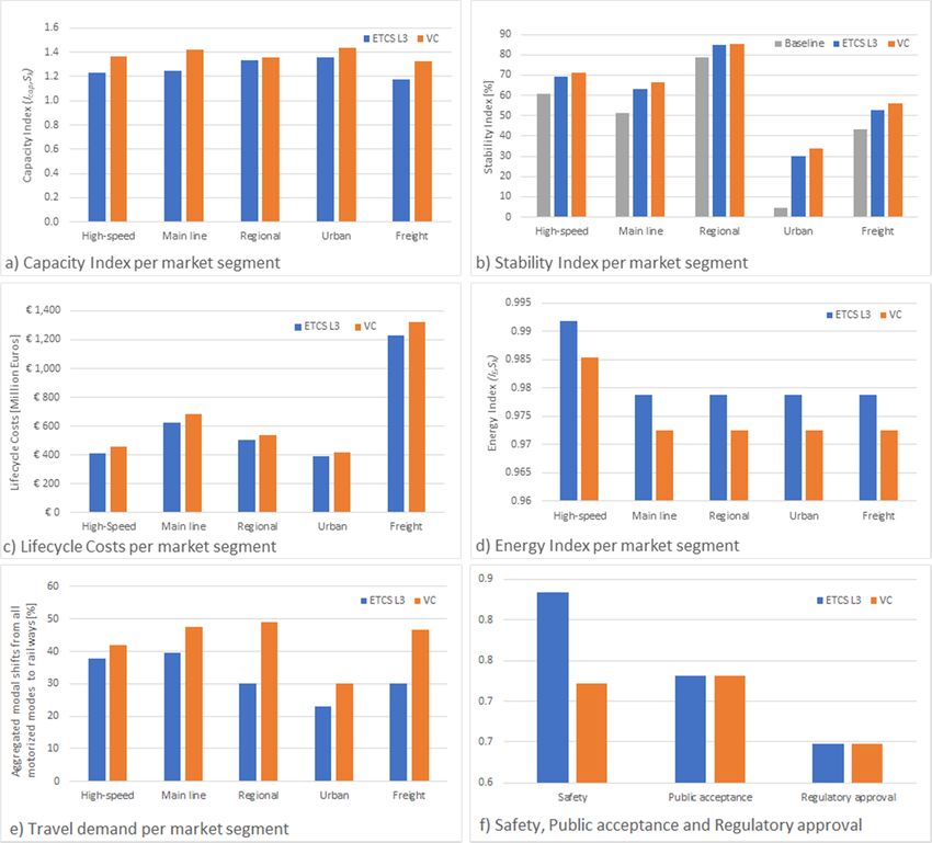
Fig. 6. Results of criteria assessment.
13J. Aoun et al. Transportation Research Part C 129 (2021) 103250
Table 4
Headway times of the operational scenarios and their change for different signalling systems compared to current technology.
Minimum headway times per market segment (s)
Market segment High-Speed Mainline
Manoeuvres Plain Merging Diverging Plain Merging Diverging
Stopping patterns ✓ ⨯ ✓ ⨯ ✓ ⨯ ✓ ⨯ ✓ ⨯ ✓ ⨯
Baseline 481.2 134.9 418.4 99.5 205.9 80.7 182.5 62.3 191 72.4 56.1 55.8
ETCS L3 334.1 74 332.2 92.3 200.9 75.7 133.2 46.5 125.8 56.2 53.3 53.1
VC 329.8 11.4 326.1 92.3 200.9 75.7 130.2 12.3 120.1 56.2 53.3 53.1
Minimum headway times per market segment (s)
Market segment Regional Urban Freight
Manoeuvres Plain Merging Diverging Plain Plain Merging Diverging
Stopping patterns ✓ ✓ ✓ ✓ ✓ ⨯ ✓ ⨯ ✓ ⨯
Baseline 156 163.1 64.3 114.4 350.1 103.4 357.4 114.9 212.4 90.1
ETCS L3 112.5 105 56.8 84.2 284.4 81.8 270.1 86.2 211.4 89.1
VC 110.7 100.4 56.8 79.6 276.9 27.2 258.2 86.2 211.4 89.1
✓: Stopping trains
⨯: Non-stopping trains
5. MCA results for Moving Block and Virtual Coupling
5.1. Case studies
Five market segments are defined by the S2R JU MAAP (2015). In this paper, we consider five case studies corresponding to a
specific corridor in Europe for each of the market segments:
For high-speed: Rome-Bologna (Italy) – 305 km;
For mainline: London Waterloo-Southampton on the South West Main Line (United Kingdom) – 127 km;
For regional: Leicester-Peterborough on the Birmingham-Peterborough line (United Kingdom) – 84 km;
For urban: London Lancaster-London Liverpool Street on the London Central Line (United Kingdom) – 7 km;
For freight: Rotterdam-Hamburg (between the Netherlands and Germany) – 503 km.
The values adopted in this paper for maximum speed, block section length, three design variables (i.e. safety margin, system re
action time and setup time), and three headway variables (i.e. turnout branch speed, turnout length and dwell time) are displayed in
Table 3 for each market segment. The system configurations represent the migration from the baseline signalling system S0 (ETCS L2
for high-speed and 3-aspect block signalling otherwise) to either ETCS L3 (Signalling alternative S1 ) or VC (Signalling alternative S2 ).
In our study, we have made the assumption to have the same safety margins for both MB and VC to keep the capacity comparison of
these two signalling systems consistent. In this way, we were able to assess the impact of the reduction in train separations just due to
the transition from an absolute braking distance in MB to a relative braking distance under VC, while keeping the same SM. The design
variables are assumed and used to analyse the operational scenarios defined in Section 4 whilst the other parameters are input for the
infrastructure capacity computation.
5.2. Criteria assessment per market segment
5.2.1. Infrastructure capacity
The method from Section 4.1.1 was used to calculate the capacity gain for VC for each manoeuvre. The calculation was done via the
headway times with the maximum utilization of the infrastructure. The decisive point in the time-distance diagram was determined for
the headway times (Fig. 5). The outcome of this procedure is a compressed path-time calculation of two trains in one operational
scenario without any buffer time. All results should be considered carefully since the infrastructure in front and behind the manoeuvres
was neglected.
Fig. 6a compares the capacity indexes of ETCS L3 MB and VC per market segment based on Equation (7). VC provides relevant
capacity improvements over MB for mainline railways (+14%), freight lines (+13%) and high-speed (+11%). VC would have a
positive homogenising effect on mainline railways due to the possibility for trains to follow each other in synchronised platoons. For
high-speed railways, VC can provide significant capacity benefits for following train movements. However, headway reductions due to
VC are only marginal (in the order of 10 s) with respect to ETCS L3, if stopping high-speed trains on a plain line are separated by a
relative braking distance. Significant headway reductions (up to 1 min) are instead observed when high-speed trains can move syn
chronously at a quasi-constant separation in a coupled platoon, as the headway comparison between VC and ETCS L3 shows for the
plain line manoeuvre with non-stopping trains (Table 4). Train platooning can be also particularly beneficial for freight trains which
usually have non-stopping operations. Despite the relatively low running speeds, VC can still provide capacity gains over MB thanks to
14You can also read