Trivariate Spline Representations for Computer Aided Design and Additive Manufacturing1 2
←
→
Page content transcription
If your browser does not render page correctly, please read the page content below
Trivariate Spline Representations for Computer Aided
                                                    Design and Additive Manufacturing1 2
                                                        Tor Dokken, Vibeke Skytt and Oliver Barrowclough
arXiv:1803.05756v3 [math.NA] 30 Aug 2018

                                                            SINTEF, P.O. Box 124 Blindern, 0314 Oslo, Norway

                                           Abstract
                                           Digital representations targeting design and simulation for Additive Man-
                                           ufacturing (AM) are addressed from the perspective of Computer Aided
                                           Geometric Design. We discuss the feasibility for multi-material AM for B-
                                           rep based CAD, STL, sculptured triangles as well as trimmed and block-
                                           structured trivariate locally refined spline representations. The trivariate
                                           spline representations support Isogeometric Analysis (IGA), and topology
                                           structures supporting these for CAD, IGA and AM are outlined. The ideas
                                           of (Truncated) Hierarchical B-splines, T-splines and LR B-splines are out-
                                           lined and the approaches are compared. An example from the EC H2020
                                           Factories of the Future Research and Innovation Actions CAxMan illustrates
                                           both trimmed and block-structured spline representations for IGA and AM.
                                           Keywords: Additive Manufacturing, Isogeometric Analysis, Computer
                                           Aided Geometric Design, Trivariate CAD, Locally Refined Splines,
                                           Topology Structures for CAD
                                           PACS: 02.60.Lj, PACS 02.60.-x
                                           2000 MSC: 65D17, 65D07, 65M60, 65M99

                                           1. Introduction
                                               Today, the additive manufacturing industry is enjoying a boom and the
                                           potential impact of AM in the coming years is enormous. The direct market
                                           for AM is expected to be $20 billion by 2020 (McKinsey) [9]. By 2025 the

                                              1  c This manuscript version is made available under the CC-BY-NC-ND 4.0 license
                                           https://creativecommons.org/licenses/by-nc-nd/4.0/
                                              2
                                                https://doi.org/10.1016/j.camwa.2018.08.017

                                           Preprint submitted to Elsevier                                      August 31, 2018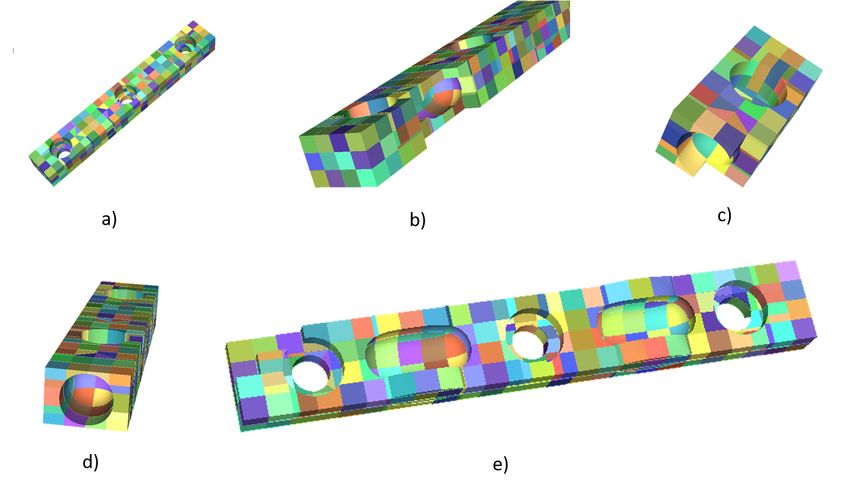
overall economic impact created by AM is expected to be much higher; reach-
ing $100 billion to $250 billion if the industrial implementation continues at
the current rate. However, one of the bottlenecks in the adoption of AM is
the lack of good tools for design and simulation that address AM directly.
    AM is a true born child of digitalization that combines aspects of mathe-
matics, material science, computational sciences and process planning. The
ISO/ASTM 5290 [12] standard defines additive manufacturing (AM) as a
process of joining material to make parts from 3D model data, usually layer
upon layer, as opposed to subtractive manufacturing and formative manufac-
turing technologies.
    The mathematical and computational communities have until recent years
paid little attention to AM, and consequently AM technology and research
have been addressed mainly from the perspectives of manufacturing and ma-
terial research. A consequence of this is that the mathematical approaches of
Computer Aided Geometric Design (CAGD) from the 1980s still dominate
AM, as described in Section 2. In Section 3 we recap univariate B-splines
space and tensor product B-splines and use this in Section 4 to address spline
spaces spanned by collections of tensor product B-splines. Then (Truncated)
Hierarchical B-splines, T-splines and LR B-splines are compared in Section
5. In Section 6 we consider how these novel spline representations can be
used in ISO 10303 STEP. The applicability of IGA for analysis based design
is discussed in Section 7, and an example of block structured and trimmed
IGA provided. How to detrim these models for quadrature is addressed in
Section 8. In Section 9 we address why the approaches outlined in the other
sections are not sufficient for the representation of lattice structures.

2. Standards and object representation for AM
    The dominant object representations in AM today focus on the needs
of manufacturing. Thus, an approximation of the smooth geometric shapes
arising in CAD is acceptable if the manufacturing tolerances of the AM-
process are respected. In the early days of AM, the STL-format emerged,
see Section 2.2. STL is based on triangulations and targets single material
AM. STL is an intermediate and simplified step between B-rep CAD-models
(addressed in Section 2.1) and the additive manufacturing process.
    In 2015 the ISO/ASTM 529 Additive Manufacturing File Format (AMF)
was introduced providing more accurate shape representation and possibil-
ities of multi-material printing, see Section 2.3. However, neither STL nor

                                      2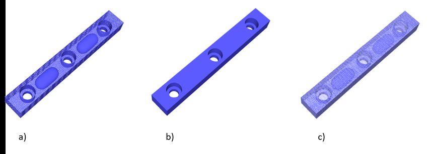
AMF are well aligned with the representation formats of CAD and Finite
Element Analysis (FEA). This lack of interoperability makes it very hard
to transfer modifications of an object done during the AM process planning
back to CAD and analysis-based design.

2.1. B-rep based CAD and STEP
    When the first 3D printing company, 3D Systems Inc, introduced their
Stereolithography technology (SLA) in 1987 [28], solid B-rep CAD was emerg-
ing [11]. B-rep CAD represents a solid object by its limiting surfaces as it
is assumed that the material of the object is uniform. In B-rep CAD, the
surface types used are elementary surfaces (e.g., planes, spheres, cones, cylin-
ders, tori) and Non-Uniform Rational B-splines (NURBS). These matched
well the subtractive and formative manufacturing process used by industry
in the 1980s.
    Data exchange of B-rep CAD models is today mainly by ISO 10303 Au-
tomation systems and integration - Product data representation and exchange
(STEP) or through vendor proprietary formats. The development of STEP
started in the 1980s, with the intent to make STEP a successor of standards
such as IGES, SET and VDA-FS. In 1994/95 ISO published the initial re-
lease of STEP as an international standard, thus ending the first phase of
the STEP development. STEP is today a widely used standard for exchange
of CAD-models and is under continuous development. In 2018 additions ad-
dressing trivariate spline representations are expected to be published. These
additions can potentially be used as resources for representing object models
addressing graded, multi and anisotropic material.

2.2. STL
    The Stereolithography technology (SLA) targets objects composed of a
single material. Thus B-rep based CAD-models in principle matched the
needs of SLA. In SLA, as well as many other additive processes, each layer
is a plane. Consequently, the 3D model data has to be repeatedly sliced by
planes. It is algorithmically simpler to slice 3D model data represented by
triangulations than the 3D model data using many smooth shape representa-
tions. The algorithmic complexity of the slicing is reduced by first tessellating
the 3D model data, and then slicing the resulting triangulated model. To
represent tessellated models 3D Systems Inc in 1987 introduced the STL-
format Standard Triangle Language, which still today is dominant for AM
shape representation. To print objects with high quality, the accuracy of the

                                       3
tessellated model must be adapted to the accuracy of the AM technology
used. In addition, the accuracy depends on the scale the object is printed at.
An STL file consists only of a list (or soup) of triangles. Each triangle (facet)
is represented by its three corners, and an optional normal assigned to the
facet. The normal is frequently set to (0,0,0), in which case it is assumed
that the direction of the normal can be inferred from the orientation of the
vertices of the triangle. There is no guarantee in STL that the collection
of triangles represents the closed surface of a volume. Though other tessel-
lation formats such as OBJ, PLY and OFF partially solve this problem by
including topology information, other issues with these tessellation formats
exist. Although STL works well for moderately complex objects with sin-
gle material AM-processes, for objects exhibiting complexity over multiple
scales, STL-files are well known to be too voluminous for efficient use. It is
worth noting that AM is particularly well suited to fabricating models with
multiscale complexity, so this issue represents a true bottleneck in the AM
pipeline today.
2.3. ISO/ASTM 529 - AMF
The AM community is aware that more advanced representations are
needed, e.g., for supporting multi-material processes and complex lattice
structures. For getting a more compact representation of sculptured shapes
AMF has introduced a curved triangle patch defined by vertices with optional
normals. Sculptured triangles are to be recursively subdivided into four
triangles to generate a set of flat triangles to reach the desired resolution.
The sculpted triangles are used for describing the surface of the volumes and
each volume can be associated with a material ID. An object can consist
of a set of volumes each with possible different material IDs. AMF gives
requirements that ensure that the geometry represented is well defined. This
will drastically improve the quality of model exchange compared to STL.
However, as of 2018 the uptake of AMF is slow.
3. Recap of some B-splines basics
As we will use properties of univariate splines spaces and tensor product
B-splines we provide some basics on these topics respectively in Section 3.1
and 3.2.
43.1. Univariate splines
Spline representations are popular for curves as they can represent com-
plicated shapes by a sequence of polynomial pieces. They are easy to evaluate
meaning that they are suitable for interactive visualization and can thereby
support design processes. The continuity between adjacent pieces can be set
as required and can be varied according to needs. For many purposes splines
of degree three are used. However, the polynomial degree can be chosen
according to what is needed for the problem addressed.
The B-spline basis, Bi,p (t), i = 1, . . . , N , is very efficient for representing
piecewise polynomial curves. It is more accurate than alternative representa-
tions, e.g., the representation of each polynomial segment in the power basis.
B-splines are defined by a non-decreasing sequence of real numbers denoted
knots t = {t1 , ..., tN +p+1 }. Here p ≥ 0 is the polynomial degree, N is the
dimension of the spline space, and ti < ti+p+1 , ∀i. The value of the B-spline
is calculated by the recursion relation
(
1, ti ≤ x < ti+1 ,
Bi,0 (x) :=
0, otherwise,
(1)
(x − ti ) (ti+p+1 − x)
Bi,p (x) := Bi,p−1 (x) + Bi+1,p−1 (x).
(ti+p − ti ) (ti+p+1 − ti+1 )
The continuity at each unique knot value is p − m where m is the mul-
tiplicity, i.e., the number of times thePknot value is repeated. If we want
N
to refine a polynomial curve f (t) = i=1 ci Bi,p (t) by inserting new knots
in the knot sequence t then the coefficients for representing f (t) in the re-
fined basis are efficiently calculated by combining weights calculated by the
Oslo-algorithm [3] and the original coefficients of f (t).
3.2. Tensor product B-spline
Definition 1.2 in [5] addresses tensor product B-splines. The focus is in
single tensor product B-splines and is thus concerned only with the knots
in the support of the univariate B-splines multiplied, not the complete knot
vector spanning univariate spline spaces.
Definition 3.1. Tensor product B-splines. Let d be a positive integer,
suppose p = (p1 , . . . , pd ) has nonnegative integer components, and let tk :=
(tk,1 , . . ., tk,pk +2 ) be nondecreasing sequences (of knots) k = 1, . . . , d. We
5define a tensor-product B-spline B[T ] = B[t1 , . . . , td ] : Rd → R from
univariate B-splines B[tk ] by
d
Y
B[t1 , . . . , td ](x1 , . . . , xd ) := B[tk ](xk ).
k=1
The support of B is given by the cartesian product
supp(B) := [t1,1 , t1,p1 +2 ] × · · · × [td,1 , td,pd +2 ]. (2)
4. Spline spaces spanned by collections of tensor product B-splines
A collection of tensor product B-splines will span a spline space. B-
spline surfaces in CAD are spanned by a special class of collections of tensor
product B-splines. The collection is generated by a tensor product of two
univariate spline spaces. Consequently, both B-splines and control points are
structured in a regular grid. The regular grid structure was essential when
B-splines were introduced in CAD in the 1980s. The tensor product structure
of the spline spaces allowed the implementation of very efficient algorithms
for interpolation, and evaluation. However, this efficiency comes at the cost
of large data increases as the size of the problems increases (both in extent
and dimension), as will be discussed later.
Spline spaces that are a tensor product of two univariate spline spaces are
central for surface representation in CAD. This relates both to tensor prod-
uct B-spline surfaces and Non-Uniform Rational B-spline surfaces (NURBS).
However, as explained in Section 4.1 such spline spaces lack local refinement.
The lack of local refinement is even more severe in the trivariate than in the
bivariate case. In AM, trivariate representations are needed when modelling
variable material properties and interior structures. Due to the lack of lo-
cal refinement of these representations, there is a demand for more flexible
collections of multivariate tensor product B-splines to describe volumes.
Industrial uptake for an augmented B-spline technology based on more
general collections of tensor product B-splines is expected to depend on its
compatibility with tensor product B-spline surfaces in CAD. The choice of
an augmented spline technology is also feasible to address from the compu-
tational perspective. Since the 1960s we have had a doubling in the number
of components per integrated circuit every 12 to 18 months (Moore’s law).
This has in practice given a similar increase in computational power. This
computational power allows augmented spline technologies to be explored.
6Figure 1: To the left the knotlines of a bi-degree (3,3) uniform tensor product B-splines
space at level l0 with the support of a sample B-spline. In the middle knotlines and a
sample B-splines at level l0 + 1, and to the right knotlines and a sample B-splines at level
l0 + 2.
With the above in mind, it seems natural to impose the following re-
quirements on refinement processes for generating more general collections
of tensor product B-splines:
• The starting point is a collection of tensor product B-splines gener-
ated by the tensor product of univariate B-spline spaces. These spline
spaces are known to span the full polynomial space over each element
(polynomial segment).
• The refinement process creates a nested sequence of refinement spaces.
The nesting of the spline spaces will ensure that the full polynomial
space is spanned also over each element in the refinement spaces.
We will discuss three approaches to refinements following the principles
above, namely, Hierarchical B-splines, T-splines and LR B-splines. These
will respectively be addressed in Sections 4.2, 4.3 and 4.4. It should be noted
that all the possible spline spaces that can be spanned over box-partitions or
T-meshes, cannot be represented by collections of tensor product B-splines.
The restriction to spline spaces that can be spanned by a collection of B-
splines is computationally feasible and builds on the B-spline technology of
state-of-the-art CAD. Alternative approaches to locally refinable splines can
be found in [19].
7Figure 2: To the left the first mesh from Fig. 1 with a region that we want to refine with
tensor product B-splines from the middle mesh in Fig. 1. The second mesh from the
left shows the mesh resulting from this refinement. Then in the third mesh a region is
marked where we want another level of refinement. The mesh to the right shows the final
hierarchical mesh.
4.1. Spline spaces spanned by a tensor product of univariate B-spline spaces
lack local refinement
Traditionally sculptured surfaces in CAD are smooth with limited local
variation and not too many degrees of freedom. Consequently, defining a
bivariate B-spline basis as a tensor product of two univariate B-spline bases
gives an efficient representation. Tensor product B-spline surfaces have been
eagerly adopted as a suitable spline representation for sculptured surfaces in
CAD. If an extra degree of freedom is needed in the first parameter direction
of a tensor product B-spline surface, an extra knot s is inserted. If the surface
originally had N1 × N2 control points, then the resulting refined surface will
have N2 additional control points. If the extra degree of freedom is needed all
along the knot line corresponding to s then the growth by N2 control points
is very reasonable. However, if the extra degrees of freedom are only need
very locally then the growth is unacceptable.
Moving to R3 the issue becomes even more apparent and more server.
Let us assume we have a volume spanned by a spline space that is the tensor
product of three univariate B-spline spaces respectively of dimension N1 , N2
and N3 . The collection will contain N1 × N2 × N3 tensor product B-splines
and control points. If we insert an extra knot in the first univariate B-spline
space, the number of tensor product B-splines and control points will grow by
N2 × N3 . While the tensor product B-splines can be represented efficiently
due to the tensor product of univariate splines space, the coefficients will
all have be to be represented, and the corresponding increase in degrees of
freedom adds computational complexity, e.g., when solving matrix equations.
8This lack of local refinement hinders spline spaces that are tensor products
of univariate spaces to be used in AM.
4.2. Hierarchical B-splines
Hierarchical B-splines (HB) were introduced in 1988 [7]. They are based
on a dyadic sequence of grids determined by scaled lattices ( k21l , k22l , . . . , k2dl ).
On each of the dyadic grids a tensor product B-spline space with uniform
knots is defined as illustrated in Fig. 1.
The refinement is done level by level by removing tensor product B-splines
on the coarser level and adding B-splines at the finer level in such a way that
linear independence is ensured [18], and the the full polynomial space is
spanned over each polynomial element. For an example of refined meshes
see Fig. 2. A partition of unity basis was provided in 2012 when Truncated
Hierarchical B-splines (THB) were introduced [8]. THB-splines provide a
basis that is a partition of unity by subtracting scaled tensor product B-
splines on the finer level from the tensor product B-splines at the rougher
level. It has been observed that some truncated B-splines risk ending up
with a support split in two disjoint parts. This problem was addressed by
imposing restrictions on allowed refinements [21]. The approach of HB and
THB is easily extended to higher dimensions, and any polynomial degree.
4.3. T-splines
When T-splines were introduced in 2003 the idea was to provide the
designer with new interactive tools for local refinement of B-splines surfaces.
Isogeometric Analysis introduced in 2005 [10] replaced the traditional shape
functions of finite elements with B-splines that cross element boarders. It was
soon evident that spline spaces made by tensor products of univariate spline
spaces were at risk of growing too large for efficient use in IGA. Consequently
T-splines gained interest from the IGA community.
T-splines denote a class of locally refined splines, in literature most often
presented as bi-degree (3, 3), that are refined by successively inserting control
points and edges in a so-called T-mesh. The starting point for T-spline
refinement is a bi-degree (3, 3) tensor product B-spline surface with control
points and knot values organized in a visual rectangular mesh as shown in
Fig. 3. In Fig. 4 we show how this graphical representation can be used
for finding the knot values of the tensor product B-spline anchored to each
control point. Then in Fig. 5 we insert two new control points and connect
these with a line making two T-joints. This illustrates how the rule from
9Figure 3: Different visualizations of the structure of a bi-degree (3,3) B-spline surface.
To the left we show the control points of the B-spline surface, and in the middle the
piecewise polynomial structure and knotlines. To the right the control points and knotlines
are combined into one graphical representation with no explicit information on knot-
multiplicity. We will use the graphical representation to the right in Fig. 4 and Fig. 5 to
illustrate the idea behind local refinement of T-splines. Note that the pair of middle knots
of each tensor product B-spline is anchored at a control point.
Fig. 4 can be used for finding the knot values of the tensor product B-splines
anchored to each of the two new control points. At each of these control
points the new line ends at an existing line forming a T-shape. The name
T-mesh comes from the T-joints created during such refinement. However,
as Fig. 7 shows, for standard T-splines also L-shapes can occur.
The above procedure is algorithmic and there is no guarantee that nested
spline spaces result from the refinement. To ensure that the spline spaces
generated are nested additional rules are imposed, defining subclasses of T-
splines. In Subsection 4.3.1 we will address Standard T-splines and in Sub-
section 4.3.2 we will address Semi-standard B-splines. Both these classes
create nested spline spaces, and a collection of B-splines that form a (scaled)
partition of unity. T-splines that do not form a scaled partition of unity
are denoted Non-standard T-splines. For such T-splines partition of unity is
achieved by rational scaling.
Linear dependence issues detected in [2] were avoided by introducing fur-
ther restrictions on allowed refinements that introduced the subclass of T-
splines denoted Analysis Suitable T-splines (AST) [22].
T-splines can be directly extended to any odd polynomial degrees, but for
10Figure 4: The figure to the left shows that we can identify the knots of the B-spline
anchored at (s3 , t3 ) by traversing the T-mesh two lines to the left, two lines to the right,
two lines down and two lines up. To the right we show the same for the B-spline anchored
at (s6 , t5 ).
even degrees there is no natural middle knot of a B-spline. To rectify this a
dual grid is introduced for the anchoring of the tensor product B-splines and
control points. The T-spline approach is also used for creating collections
of trivariate tensor product B-splines [29]. Truncation of T-splines has also
been proposed [27].
4.3.1. Standard T-splines
The first T-splines introduced were Standard T-splines [23]. The tensor
product B-splines
P created by standard T-splines form an unscaled partition
of unity, i Bi (s, t) = 1. The refinement follows three rules, where the first
relates to consistency of knot values, the second relates to when to connect
control points (as we did in Fig. 5). The third restricts when a refinement
i allowed: All existing tensor product B-splines that are to be refined must
to have identical knot vectors in the other parameter direction, see Fig. 6.
This can also be regarded as requiring a local tensor product structure on
the tensor product B-splines to be updated after insertion of a new control
point. For full details consult [23].
4.3.2. Semi-standard T-splines
When performing repeated refinement such as shown in Fig. 5 there is
no guarantee that the resulting spline space includes prior spline spaces in
the refinement sequence. Let Q, as in Fig. 7.a, be a new control point with
11Figure 5: To the left we show that we can add a new control point at (s∗ , t5 ) and then
traverse the mesh to find the knots of the new tensor product B-spline. Note that the knot
vector in the first parameter direction of the B-splines anchored at (s4 , t5 ), (s5 , t5 ), (s6 , t5 )
and (s7 , t5 ) have to be updated to take s∗ into account. These tensor product B-splines
all have anchor points with t5 in the second knot direction, and s∗ is within their interval
of knots in the first knot direction. To the right we connect the two new control points
with a line and make two T-joints, following the second rule of standard T-splines.
knot coordinate (σ, τ ) and let lτ be the constant knot line on which Q lies.
When refining, Q is used for two purposes:
1. Q is used as an anchor point for a new tensor product B-spline with
knots picked from the T-mesh.
2. The knot value τ is used for refining all B-splines with anchor points
on lτ and support in the first parameter direction containing τ .
There is no guarantee that the collection of tensor product B-splines resulting
from the above two steps match the T-mesh. (Illustrated in Fig. 7.c.) For
the B-spline in Fig. 7.c to be represented in the T-mesh a new control point
R has to be added as shown in Fig. 7.d. Now the new spline space is a
refinement of the spline space from which we started.
A refinement process such as the above ensures that we generate nested
spline spaces and generate Semi-standard T-splines. A formal algorithm for
this process is described in [24]. Below we present a condensed version of the
algorithm:
1. Insert new control points into the T-mesh.
2. Make a collection of B-splines by refining existing tensor product B-
splines using Q, and creating the tensor product B-splines anchored to
the new control points.
12Figure 6: To the left we show that for standard T-splines four adjacent control points in one
parameter direction have to be inserted before refinement is allowed in the other parameter
direction. Note that the control points all must be on the same constant parameter line.
To the right we show that a control point is inserted in the middle line segment of the line
segments created by the insertion of the four control points inserted in the mesh to the
left.
3. If any tensor product B-spline misses a knot dictated by mesh traversal,
update the tensor product B-spline by knot insertion.
4. If a tensor product B-spline has a knot that is not dictated by mesh
traversal, add an appropriate control point in the T-mesh.
5. Repeat 3. and 4. until all issues are solved.
4.4. LR B-splines
Locally Refined B-splines (LR B-splines) were introduced in 2013 [5] and
the use of LR B-splines in IGA presented in [16]. The definition of LR B-
splines is based on what is denoted box-partitions of a d-box in Rd , d ≥
1. The approach of LR B-splines is thus not restricted to the bivariate,
or trivariate case. There is no restriction on the polynomial degrees to be
used and odd and even degrees are treated in the same way. Knots can be
inserted at arbitrary values, thus supporting non-uniform refinements. The
refinement is performed by inserting a meshrectangle that splits at least one
B-spline. In the bivariate case meshrectangles are knot-line segments, and
in the univariate case they are knots. A meshrectangle can have multiplicity
higher than 1, thus generalizing knot multiplicity of univariate B-splines.
Rather than go deep into technical detail, we will illustrate the concept with
13Figure 7: In a) we insert a new control point Q in the T-mesh from Figure 9 in [24]. In
b) a B-spline to be refined with the first parameter value of Q is shown. The refinement
creates a B-spline in c) with centre knots at Q. This cannot be found by traversing the
mesh. To make this B-spline valid (and to ensure nested spline spaces) a new control
point R is added in d), and connected by line segments to existing control points. In e)
we see that the B-spline in c) can be generated from the updated mesh. In f) we see an
additional B-spline anchored in R.
examples of bi-degree (3,3) LR B-splines. For technical details, consult the
cited publications.
In Fig. 8 we show how a the parameter plane and the knot values of a
bi-degree (3,3) tensor product B-spline space is represented as a box partition
with multiplicities assigned to the mesh rectangles (knot-line segments). The
refinement of LR B-splines is illustrated in Fig. 9. The rules for LR B-spline
refinement are as follows:
• Insert a meshrectangle that splits the support of at least one B-spline.
• Find all B-splines that have a support that is split by the meshrectangle.
Refine these B-splines until the collection of B-splines contains only
14Figure 8: To the left we have the knotlines and knots of a bi-degree (3,3) tensor product
basis. In the middle the knot lines are represented as mesh rectangles with multiplicities
assigned. To the right we represent the meshrectangles of multiplicity 4 with thick lines,
and the meshrectangles of multiplicity 1 with thin lines. We will use this convention for
meshrectangle multiplicities 1 and 4 in the illustrations to follow.
minimal support B-splines. Note that existing meshrectangles might
split B-splines resulting from the refinement. Such B-splines must be
recursively subdivided until all B-splines have minimal support.
As with T-splines there are refinement configurations that can result in
a linearly dependent collection of tensor product B-splines. However, linear
independence can be ensured if a hand-in-hand refinement condition is ful-
filled throughout the refinement process. This means that the dimension of
the spline space is checked against the increase in number of B-splines at
each refinement step.
5. Comparing Hierarchical B-splines, T-splines and LR B-splines
In the previous sections we have explained the ideas behind (truncated)
hierarchical B-splines, T-splines and LR B-splines. In this section we will
try to explain how the different approaches relate. Can one method mimic
the properties of the other approaches? In Section 5.1 we will investigate
the strategies for specifying the refinement. This is followed in Section 5.2
by discussion of generalization in degree and dimension, and then in Section
5.3 the difference of spline spaces will be addressed. Linear independence is
important when doing isogeometric analysis and this is addressed in Section
5.4.
15Figure 9: On the upper left corner we have the mesh of a box-partition of a bi-degree (3,3)
tensor product B-spline basis. We insert a meshrectangle that splits at least one B-spline
over this mesh. The four meshes following to the right show the tensor product B-splines
split by this refinement. In the middle row of meshes we show how the four tensor product
B-splines are refined into five tensor product B-splines. In the left mesh on the last row we
insert one meshrectangle with multiplicity two. This only affects the B-spline highlighted
in the second mesh on the last row. The next meshes show the resulting refined B-splines.
5.1. Refinement specification
Hierarchical B-splines, T-splines and LR B-splines have different strate-
gies for specifying the refinement to be performed, respectively specification
of the region to be refined for the next hierarchical level, inserting new con-
trol points in the T-mesh, and inserting meshrectangles in the box-partition.
A natural question to pose is if these “user interfaces” can be interchanged.
• Specify region of interest for next level of hierarchical refine-
ment. As both T-splines and LR B-splines have very high flexibility
with respect to refinement it is feasible to impose a hierarchical B-spline
type of refinement rule to both methods and specify refinement level-
by-level. The tensor product B-splines to be refined can be selected
by a specification of regions as for HB/THB. For LR B-splines this
16Figure 10: To the left we show how knot values can be assigned to the control points of
tensor product B-splines of bidgree (3, 3). To the right we show how knot values can be
assigned to control points of B-splines of bidegree (2, 2) by averaging the middle knots
thus creating the Greville point of the tensor product B-spline.
hierarchical B-splines approach has been followed using what we call
structured refinement [16], where all elements of the selected B-splines
are split in two in all parameter directions at each refinement level. For
bi-degree (3,3) and lower such LR B-splines are linearly independent,
but linear dependence has been observed in degrees ≥ 4.
• Refinement by insertion of new control points in the control
point mesh. As hierarchical B-splines are intrinsically defined by
the region of subdivision, this is not a feasible approach. However, the
control point insertion of T-splines can be used for LR B-splines. In Fig.
10 to the left we show that for LR B-splines of bidegree (3,3) the control
points can be anchored to the middle knot pair of the corresponding
tensor product B-spline similar to the anchoring of control points for
T-splines. In Fig. 10 to the right we show that the control vertices
of a bidegree (2,2) tensor product B-spline/LR B-spline surface can be
assigned a parameter value pair corresponding to the Greville point.
Note that after splitting such Greville point based parameter value
pairs must be updated.
• Refinement by inserting meshrectangles. While LR B-splines
enforce that all tensor product B-splines are minimal support after
each refinement step, T-splines only enforce minimal support in the
parameter direction of the refinement, and only on the B-splines split by
17the new control point. So, the LR B-spline approach can be given a very
T-spline like behaviour if we relax the minimal support requirement to
only be in the refinement direction, and ensure that refinements are
between anchored control points.
5.2. Generalization in degree and dimension
The approach of (truncated) hierarchical B-splines and LR B-splines are
neither restricted in degree nor dimension. Both perform refinement in the
parameter domain, and all degrees are treated in the same way. As T-
splines perform refinement in the control mesh, more advanced navigation
has to take place for identifying knot values as the number of dimensions
increases. There are already examples of trivariate T-splines [29]. T-splines
are explained using bi-degree (3,3), but the anchoring of tensor product B-
splines to vertices works well for any odd degree. For even degrees the dual
grid can be used.
5.3. Differences of spline spaces for hierarchical type meshes
As the algorithms for finding which tensor product B-splines to use are
different for truncated hierarchical B-splines, T-splines and LR B-splines the
spline spaces generated will be different. However, when T-splines and LR
B-splines mimic the knotline meshes of hierarchical B-splines, the behaviour
is quite similar. In [17] it is shown that on similar grids, LR B-splines and
truncated hierarchical B-splines are fairly similar with respect to the condi-
tion numbers of the stiffness matrix for the examples considered. It must
be expected that T-splines will behave in a similar way. However, the origi-
nal formulation of hierarchical B-splines has a significantly higher condition
number due to the lack of partition of unity of the resulting B-splines. In
general, the number of tensor product B-splines will grow much faster for
(truncated) hierarchical B-splines than LR B-splines and T-splines. For LR
B-splines and T-splines a single vertex/knotline segment can be inserted,
while for (truncated) hierarchical B-splines refinements dictate that a much
higher number of knotline segments will be added. Consequently, for large
problems it much be expected that LR B-splines and T-splines will outper-
form truncated hierarchical splines.
5.4. Linear independence
Truncated Hierarchical B-splines are always linearly independent. LR B-
splines can be defined over most meshes of hierarchical B-splines (in some
18cases extra refinement is necessary). Linear independence is guaranteed for
LR B-splines of bi-degree (3,3) or lower over such hierarchical meshes. The
only example known for T-splines that is linearly dependent has multiplicity
of knot values in the interior of the mesh. Consequently, we can expect that
T-splines on meshes similar to meshes of hierarchical B-splines are linearly
independent. For LR B-splines of higher bi-degree than (3,3) on hierarchical
meshes a simple rule can be imposed on the mesh that guarantees linear
independence: if the region to be refined can be split into two overlapping
subregions whose intersection does not contain any of the B-splines to be
refined then special care has to be taken to check if the region has to be
extended to avoid linear dependence.
Due to the flexibility of LR B-splines and T-splines there are situations
where the resulting collection of tensor product B-splines are linearly depen-
dent. For bivariate LR B-splines it is always possible to use the hand-in-hand
principle mentioned above to ensure that a refinement will produce a linearly
independent set of B-splines. However, this depends on the availability of
an appropriate dimension formula, which is currently only available in the
bivariate case. Work is going on to find other subclasses of LR B-spline that
ensure linear independence without using the hand-in-hand principle. For
T-splines the subset of analysis suitable T-splines is always linearly indepen-
dent.
6. Trivariate spline extensions to ISO 10303
The development of B-spline technology in the 1970s and NURBS in
the 1980s had a rapid uptake both in CAD-industry and in the 1990s by
ISO 10303 STEP [14]. Prior representations for freeform curves and sculp-
tured surfaces were replaced by curves and tensor product surfaces based on
B-spline and NURBS technology. As the subtractive and formative manu-
facturing technologies at that time were based on uniform material there was
no need for representing the interior of an object.
Before IGA, addressed in Section 7.1, was accepted as a technology with
great industrial potential, trivariate B-spline representations for volume ob-
jects attracted little attention in STEP. The consequence was that the trivari-
ate B-spline representation already in Part 42 [15] was not described in Appli-
cation Reference Model (ARM) Part 1801 B-spline Geometry, see Appendix
B for details. The ARMs of STEP are written as a reference for those that
develop converters.
19The EC Factories of the Future project TERRIFIC (2011-2014, Contract
No. 284981) proposed several additions related to Locally Refined Splines to
STEP Part 42. In addition, extensions of STEP AP 242 Edition 2 [13] were
proposed. The extensions to Part 42 will be published in 2018. To support
the Part 42 extension the preparation of a new ARM, currently denoted
Extended B-spline Geometry, was started in 2018 in the EC Factories of
the Future project CAxMan (2015-2018, Contract No. 680448). For details
see Appendix B. To support trivariate spline representations, extensions are
needed in other parts of STEP such as Part 50 and Part 52. These extensions
are carried out by other parts of the STEP-community.
7. Analysis-based design for AM
Additive manufacturing is moving from objects composed of a single ma-
terial to objects composed of multiple discrete materials and graded materi-
als. The additive manufacturing processes create objects with material prop-
erties that are significantly more anisotropic than traditional manufacturing
technologies. Consequently, it will be beneficial to use extensive analysis al-
ready during the design stage to better support the additive manufacturing
technology chosen.
The specificities of the different additive processes have a strong influence
on how an object should be designed. For example, for metal powder bed
based additive technologies, overhangs of more than 45 degrees require sup-
port structures to be added. However, if the printing direction is known then
the “roof” of an internal void or cavity could possibly be replaced by a drop
shaped roof thus avoiding overstepping the 45-degree restriction. However,
the consequences of such design changes targeting manufacturability should
be analysed.
It is well known that meshing from CAD is work intensive. The DART
study of Sandia Labs quantified the increasing challenge of mitigating the
problems with non-watertight CAD-models when creating suitable meshes
for FEA [1]. Time spent fixing such issues was reported to have increased
from 73% in 2005 and numbers as high as 90% have been mentioned in 2017.
The large CAD vendors invest much effort to make B-rep CAD and FEA
seamlessly interoperable in their market offerings.
To go beyond what the large vendors offer, it seems that a suitable ap-
proach is to build analysis-based design for AM on a combination of trivariate
20CAD-models and IGA. Originally IGA was based on block-structured trivari-
ate spline models, an approach like CAD-models before trimming of B-spline
surfaces was introduced. To augment the trivariate spline representation it
is natural to trim the trivariate spline models by surfaces, thus generalizing
trimming of spline surfaces by loops of edges to trimming of spline volumes
by B-rep shells. This is the same line of ideas as the embedded methods of
cut-FEM and the Finite Cell Method (FCM). However, to trim the trivariate
spline model with a CAD B-rep model that is not watertight is as far as we
know new. In Section 7.2 we address the work performed in the CAxMan
project on trimmed trivariate spline models.
7.1. Isogeometric Analysis
In 2005 Tom Hughes [10] introduced Isogeometric Analysis (IGA). IGA
builds on the ideas of FEA. In FEA the shape functions of an element are
local to the element. In IGA the shape functions are replaced by B-splines,
that cross element boundaries. Thus, the same B-spline can be used as shape
function in more than one element. The transition between elements will
replicate the continuity of the B-splines used. As B-splines and Non-Uniform
Rational B-splines can represent all CAD-shapes, IGA can in principle have
an accurate representation of all shapes used in CAD-design [25]. B-splines
can have any polynomial degree, consequently IGA supports the use of higher
degree element representations in simulation. IGA has been demonstrated to
be more accurate than traditional FEA. However, making a trivariate block-
structured spline model suited for IGA from a CAD-model meets the similar
challenges to making a block-structured FEA-mesh from CAD.
Advantages and challenges of block-structured IGA (no trimming):
• Easy to handle in analysis.
• An approximation step is normally required in the block structuring
process.
• Difficult to create IGA block structured models for complex objects:
– For surfaces models there might occur vertices with valence differ-
ent from four, e.g., less than four or more than four faces connect
at a vertex.
– For surfaces models there might occur singular edges.
21Figure 11: To the left a CAD type B-rep topology data structure, and to the right a data
structure addressing the needs of a block-structured model for IGA where the blocks may
be trimmed volumes. In a B-rep model a face is unique, and the topological outline(s)
of the face is described by loop(s) of edges. When two faces are adjacent the connection
is described through relations between coincident edges of the two faces (indicated by
the 0 : 1 on the relation between edges in the left picture). In the trimmed trivariate
block-structure for IGA, two topological volumes that are adjacent are connected through
coincident faces through a relation (indicated by the 0 : 1 on the relation between faces
in the right picture). While an edge in a B-rep model can only be related to two faces,
an edge in the trimmed trivariate block-structure for IGA can be coincident to edges of
multiple faces.
– For volume models there might occur edges with valence differ-
ent from four, e.g., less than four or more than four topological
volumes connect along an edge.
– For volume models there might occur singular edges and faces.
7.2. Trimmed trivariate CAD, IGA and AM
In Fig. 11 we show to the left a typical topological structure for B-rep
CAD, and to the right a proposed topological structure for trimmed trivari-
ate CAD [25]. In the latter, two new entities are introduced: the topological
22Figure 12: In a) a transparent view showing the voids. In b) the outer shell of a CAD-
model. In c) the trimmed trivariate spline representation, where the white shadow follows
the main shape of the volume.
volume and the trivariate volume that contains the mathematical represen-
tation. This approach allows the B-rep CAD-model to trim the trivariate
volumes. Although this in principle seems simple, the difference between
what is regarded as a watertight CAD model and as a watertight FEA or
IGA-model remains.
• A CAD model is regarded as watertight if the topology representation
is correct and the gaps between adjacent faces are within user defined
tolerances.
• A FEA model is watertight when the elements match exactly, no gaps
are allowed between elements.
• A volumetric IGA model is watertight when spline volumes match ex-
actly, no gaps are allowed between adjacent volumes.
So, to trim a block-structured trivariate IGA model with B-rep CAD-
models poses algorithmic challenges. If the original B-rep model includes
gaps and these live on through subsequent uses of the model, algorithms
must always take the challenges of gaps into consideration. Alternatively, the
model must be repaired to remove gaps, and thus simplify subsequent uses.
In the CAxMan project, the focus is on trimmed trivariate block-structured
models for IGA and AM.
23Figure 13: In image a) the detrimming and reparameterization to trivariate hexahedra
shapes of the trimmed trivariate model. In b) some spline hexahedra are removed to
show the reparameterization around the void, and in c) and d) a void seen from another
direction with other spline hexahedra removed. In e) a section of the detrimming is seen
from the top.
8. Detrimming of trimmed trivariate spline models
Quadrature of a trivariate spline volume that is parameterized over a
hexahedron can be decomposed into univariate quadrature in each of the
parameter directions. Consequently, to be able to perform numerical inte-
gration over the trimmed trivariate spline model, it makes sense to split the
model into a collection of sub-volumes each parameterized over a hexahedron.
In CAxMan we have implemented a first version of such a detrimming algo-
rithm. Fig. 12.a) illustrates the conversion of a B-rep CAD-model with voids
to a trimmed trivariate spline model. This is then detrimmed for quadrature
as illustrated in Fig. 13a–e.
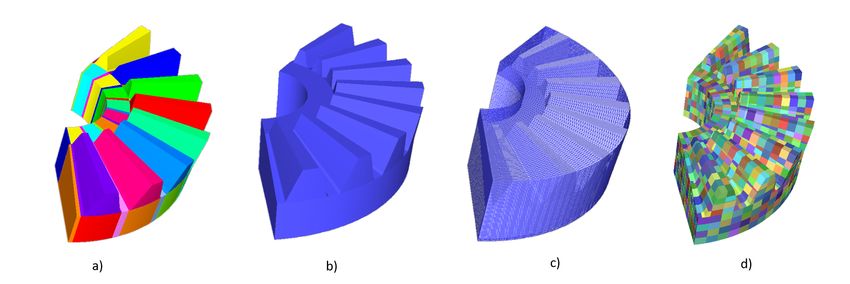
Fig. 14 illustrates for a part of a gear, a pure block-structured model as
well as a trimmed block-structured model of the part of the gear, and the
detrimming of this.
24Figure 14: In a) a block-structured model of a gear. The same gear represented as a
trimmed spline volume in b), then in c) the trimmed volume with the trimming surfaces,
and d) is the detrimming prepared for quadrature. Note that the shape of the trivari-
ate trimmed spline follows the rotational shape of the gear and thus ensures rotational
symmetry. The example is courtesy of the CAxMan partner Stam S.r.l..
9. Open challenges
To represent accurately the fine detail of objects with large interior lattice
structures, B-rep CAD is not feasible as the number of geometric elements
will be much larger than what was foreseen when this format was established.
In addition to the bulk of the number of geometric elements, geometric toler-
ances will also pose a challenge. In general B-rep based CAD-systems allow
gaps between adjacent surfaces controlled by user defined tolerances. One
solution to this is to set finer tolerances. However, then CAD models that
are valid with their original tolerance settings will be invalid with the finer
tolerances.
When designing lattice structures, the size of a gap between adjacent
faces and the thickness of the volumetric elements of the lattice structures
risk not having a proper separation. This potentially creates failure of the
CAD-system. This might be one of the reasons that lattice structures are
today frequently created after the conversion to STL, with the consequence
that the CAD-model of the object manufactured does not accurately mirror
the object manufactured.
The use of FEA or trivariate spline based CAD-model representation will
solve the tolerance problem [26] [6] [20]. However, the bulk of the represen-
tation will grow. Automatic generation of trimmed trivariate CAD-models
is still a technology under development, so there are still significant develop-
25ments necessary before it is as mature as B-rep based CAD. More innovative
approaches to lattice structure representations must be pursued in the future.
At SIM-AM in Munich in October 2017 many different promising approaches
for modelling of lattice structures were presented. However, the challenge is
to ensure that these can be represented in a CAD-based digital twin that
reflects the object manufactured by additive technology. Our feeling is that
a lot seems to remain before we have a generic technology for representation
and modelling of lattice structures for AM.
10. Acknowledgement
This project has received funding from the European Union’s Horizon
2020 research and innovation programme under grant agreement No 680448.
11. References
References
[1] Boggs, P.T., Althsuler, A., Larzelere, A.R., Walsh, E.J., Clay, R.L,,
Hardwick M.F., 2005, DART system analysis.. United States: N. p.,
Web. doi:10.2172/876325.
[2] Buffa, A., Cho, D., Sangalli, G., 2010. Linear independence of the T-
spline blending functions associated with some particular T-meshes.
Comput. Methods Appl. Mech. Engrg. 199 (2324), 1437–1445.
[3] Cohen, E., Lyche, T., Riesenfeld, R.R., 1980. Discrete B- splines and
subdivision techniques in computer-aided geometric design and com-
puter graphics, Computer Graphics & Image Processing, Vol.14(2), 87–
111.
[4] Dokken, T., Skytt, V., Haenisch, J., Bengtsson, K., 2009. Isogeometric
representation and analysis: bridging the gap between CAD and anal-
ysis. In: 47th AIAA Aerospace Sciences Meeting Including The New
Horizons Forum and Aerospace Exposition. 58 January 2009, Orlando,
Florida. American Institute of Aeronautics and Astronautics.
[5] Dokken, T., Lyche, T., Pettersen, K. F., 2013. Polynomial splines over
locally refined box-partitions, Computer Aided Geometric Design, Vol-
ume 30 (3), 331–356.
26[6] B. Ezair, B., Elber, G, 2017. Fabricating Functionally Graded Material
Objects Using Trimmed trivariate Volumetric Representations. Proceed-
ings of SMI’2017 Fabrication and Sculpting Event (FASE), Berkeley,
CA, USA, June 2017.
[7] Forsey, D. R., Barrels, R. H., 1988. Hierarchical B-Spline Refinement,
Comput. Graphics, 22, 205212.
[8] Giannelli, C., Jttler , B., Speleers, H., 2012. THB-splines: The truncated
basis for hierarchical splines, CAGD 29(7), 485–498.
[9] https://www.mckinsey.com/business-functions/operations/our-
insights/additive-manufacturing-a-long-term-game-changer-for-
manufacturers.
[10] Hughes, T.J.R., Cottrell, J.A.,Bazilevs, Y., 2015. Isogeometric analysis:
CAD, finite elements, NURBS, exact geometry, and mesh refinement,
Comput. Methods Appl. Mech. Engrg., 194, 4135 – 4195.
[11] Implementation of APS-Sculpured Surfaces in the CAD/CAM Systems
CDM300 and Technovision in Advance Production Sytem - CAD/CAM
of the Future, Editor Ø. Bjørke, Tapir Publisher, Trondheim, Norway,
1987, 184–207.
[12] ISO/ASTM 52900:2015 (ASTM F2792), Additive manufacturing – Gen-
eral principles – Terminology, 2015.
[13] ISO/DIS 10303-42:2015, Industrial automation systems and integration
Product data representation and exchange Part 42: Integrated generic
resource: Geometric and topological representation.
[14] ISO 10303-28:2007, Industrial automation systems and integration
Product data representation and exchange Part 28: Implementation
methods: XML representations of EXPRESS schemas and data, using
XML schemas.
[15] ISO 10303-42:2016, Industrial automation systems and integration
Product data representation and exchange Part 42: Integrated generic
resource: Geometric and topological representation.
27[16] Johannessen, K.A., Kvamsdal, T., Dokken, T., 2014. Isogeometric anal-
ysis using LR B-splines, Computer Methods in Applied Mechanics and
Engineering 269, 471–514.
[17] Johannessen,K.A., Remonatol, F. , K.A., Kvamsdal, 2016. On the sim-
ilarities and differences between Classical Hierarchical, Truncated Hi-
erarchical and LR B-splines, Computer Methods in Applied Mechanics
and Engineering 291, 64-101.
[18] Kraft, R., 1998. Adaptive und linear unabhangige multilevel B-splines
und ihre Anwendungen, PhD thesis, Math Inst A, University of
Stuttgatt.
[19] Li, X., Chen, F.L., Kang, H. M., et al., 2016 A survey on the local
refinable splines. Sci. China. Math.,59, 617–644, doi: 10.1007/s11425-
015-5063-8.
[20] Massarwi, F., G. Elber, G., 2016. A B-spline based Framework for Vol-
umetric Object Modeling. CAD 78, 36–47.
[21] Mokri, D., Jttler, B., Giannelli., C., 2014. On the completeness of hier-
archical tensorproduct B-splines. Journal of Computational and Applied
Mathematics, 27, 53–70.
[22] Scott, M.A., Li, X., Sederberg, T.W., Hughes, T.J.R., 2012. Local re-
finement of analysis-suitable T-splines, Computer Methods in Applied
Mechanics and Engineering, Volumes 213–216, 206–222.
[23] Sederberg, T. W., Zheng, J., Bakenov A., Nasri A., 203. T-splines and
T-NURCCs. ACM Transactions on Graphics 22, 3, 477–484.
[24] Sederberg, T. W., Cardon, D. L., Finnigan, G. T., North, N. S., Zheng,
J., and Lyche, T., 2004 . T-spline simplification and local refinement.
ACM Trans. Graph. (TOG), 23 , 276–283.
[25] Skytte, V., Dokken, T., 2016. Models for Isogeometric Analysis from
CAD, in IsoGeometric Analysis: A New Paradigm in the Numerical Ap-
proximation of PDEs, , Buffa, A., Sangalli, G. (Eds.), C.I.M.E. Lecure
Notes in Mathematics 2161, Springer, 71–86.
28[26] Weeger, O., Kang, Y.; Yeung, S.-K., Dunn, M. L., 2016. Optimal De-
sign and Manufacture of Active Rod Structures with Spatially Variable
Materials, 3D Print. Addit. Manuf. 3(4), 204–215.
[27] Wei, X., Zhang, Y. J., Liu,L. , Hughes,T. J. R. . Truncated T-splines:
Fundamentals and Methods. Computer Methods in Applied Mechanics
and Engineering Special Issue on Isogeometric Analysis, 316:349-372,
2017.
[28] Wohlers, T., Gornet, T., 2014. History of additive manufacturing, in
Wohlers Report 2014, Wholers associates.
[29] Zhang, Y., Wanga, W., Hughes, T. J.R, 2012. Solid T-spline construc-
tion from boundary representations for genus-zero geometry, Computer
Methods in Applied Mechanics and Engineering, Volumes 249252, 185–
197.
Appendices
Extensions to ISO 103030 (STEP)
A. Application Reference Model 1801: B-spline Geometry
ARM 1801 includes the following well know representations of geometry
using B-splines:
• B-spline curve.
• B-spline surface.
• Rational B-spline curve.
• Rational B-spline surface.
• Surface with explicit knots.
• Surface with implicit knots.
29B. Proposal for new ISO 10303 Application Reference Model: Ex-
tended B-spline Geometry
The ARM to be proposed on Extended B-spline Geometry is planned to
include:
• B-spline volume and B-spline volume with knots. Although
these have been part of Part 42 for a long time, an ARM description
has not been made until now, probably due to little interest in its use
before IGA emerged. This is a parametric volume represented by a
trivariate tensor product spline basis.
• Status of linear independence is important for LR B-splines and
T-splines. The values this variable can have are Independent, Not in-
dependent, and Not tested.
• List of types of Locally Refined Splines. The list of values for
this variable currently includes Analysis Suitable T-spline, Hierarchical
B-spline, LR B-spline, Semi-Standard T-spline and Standard T-spline.
The Truncated Hierarchical B-splines are currently not included but
can potentially be represented by expanding the truncation and assign-
ing the vertex values to all vertex values used, including the occurrences
used in the truncation. This will result in multiple occurrences of the
same B-spline as all its occurrences will be explicitly represented.
• Local B-spline. As both Hierarchical B-splines, T-splines and LR
B-splines are based on collections of (tensor product) B-splines with
control points and scaling factors, each individual (tensor product) B-
spline has to be represented as an entity. Each (tensor product) B-
spline entity points for each dimension to a list of knot values with a
parallel list of multiplicities.
• Locally refined spline curve and rational locally refined spline
curve. This entity allows us to extracted constant parameter line
spline curve from a locally refine spline surface of volume represented
by B-splines from the locally refine spline surface of volume. In general,
this description will not be a minimal support set of B-splines, and
will be represented by a collection of B-splines that risk being linearly
dependent. However, these spline curves can be exactly converted to a
30(Rational) B-spline curve that is using a linearly independent collection
of B-splines when necessary.
For many uses it can often be wise to convert the curve to a minimal
support B-spline basis, i.e., a B-spline basis using a normal knot vector.
• Locally refined spline surface and rational locally refined spline
surface can be of types listed in List of types of Locally Refined Splines.
The surface is represented by a collection of bivariate tensor product
B-splines with scaling factors and control point values.
• Locally refined spline volume and rational locally refined spline
volume can be of types in List of types of Locally Refined Splines.
The volume is represented by a collection of trivariate tensor product
B-splines with scaling factors and control point values.
31You can also read