Turnout in the Municipal Elections of March 2020 and Excess Mortality during the COVID-19 Epidemic in France - IZA DP No. 13335 JUNE 2020
←
→
Page content transcription
If your browser does not render page correctly, please read the page content below
DISCUSSION PAPER SERIES

IZA DP No. 13335

Turnout in the Municipal Elections of
March 2020 and Excess Mortality during
the COVID-19 Epidemic in France

Simone Bertoli
Lucas Guichard
Francesca Marchetta

JUNE 2020
DISCUSSION PAPER SERIES

IZA DP No. 13335

Turnout in the Municipal Elections of
March 2020 and Excess Mortality during
the COVID-19 Epidemic in France
Simone Bertoli
Université Clermont Auvergne, CNRS, CERDI, IUF and IZA
Lucas Guichard
IAB, Université Clermont Auvergne, CNRS and CERDI
Francesca Marchetta
Université Clermont Auvergne, CNRS and CERDI

JUNE 2020

Any opinions expressed in this paper are those of the author(s) and not those of IZA. Research published in this series may
include views on policy, but IZA takes no institutional policy positions. The IZA research network is committed to the IZA
Guiding Principles of Research Integrity.
The IZA Institute of Labor Economics is an independent economic research institute that conducts research in labor economics
and offers evidence-based policy advice on labor market issues. Supported by the Deutsche Post Foundation, IZA runs the
world’s largest network of economists, whose research aims to provide answers to the global labor market challenges of our
time. Our key objective is to build bridges between academic research, policymakers and society.
IZA Discussion Papers often represent preliminary work and are circulated to encourage discussion. Citation of such a paper
should account for its provisional character. A revised version may be available directly from the author.

                                                     ISSN: 2365-9793

                                           IZA – Institute of Labor Economics
Schaumburg-Lippe-Straße 5–9                      Phone: +49-228-3894-0
53113 Bonn, Germany                             Email: publications@iza.org                                    www.iza.org
IZA DP No. 13335 JUNE 2020
ABSTRACT
Turnout in the Municipal Elections of
March 2020 and Excess Mortality during
the COVID-19 Epidemic in France*
We analyze the consequences of the decision of French government to maintain the
first round of the municipal elections on March 15, 2020 on local excess mortality in the
following weeks. We exploit heterogeneity across municipalities in voter turnout, which
we instrument using a measure of the intensity of local competition. The results reveal that
a higher turnout was associated with a significantly higher death counts for the elderly
population in the five weeks after the elections. If the historically low turnout in 2020 had
been at its 2014 level, the number of deaths would have been 21.8 percent higher than
the one that was recorded. More than three quarters of these additional deaths would have
occurred among the individuals aged 80 and above.
JEL Classification: J11, D72
Keywords: COVID-19, excess mortality, voter turnout, intensity of electoral
competition, municipal-level data
Corresponding author:
Simone Bertoli
CERDI
Avenue Leon-Blum, 26
F-63000 Clermont-Fd
France
E-mail: simone.bertoli@uca.fr
* The Authors are grateful to Paolo Brunori, Jesús Fernández-Huertas Moraga, Bruno Meunier and Hillel Rapoport
for their comments, and to Olivier Santoni for providing excellent research assistance, and they acknowledge the
support received from the Agence Nationale de la Recherche of the French government through the program
“Investissements d’avenir” (ANR-10-LABX-14-01); the usual disclaimers apply.“[I] have asked the advice of scientists about our local elections,
whose first round will be held in a few days. They believe that nothing goes against the fact that the
French citizens, even the most vulnerable among them, go to the polling stations.”
(Speech of the French President Emmanuel Macron, March 12, 2020).1
1 Introduction
European countries have been confronted, in the early phases of the COVID-19 epidemics,
with challenging decisions concerning the timing and the extent of the introduction of the
social distancing measures that were recommended to slow down the diffusion of the virus.
The French government faced a particularly difficult situation, as all municipalities had to
renew their councils and mayors in a two-round election that was scheduled on March 15
and 22, 2020. The lack of support from the opposition, which even referred the scenario of
postponing the elections as a coup d’État,2 eventually induced the decision to maintain the
first round.3 The President Emmanuel Macron made a speech on March 12, describing the
epidemics as the “biggest health crisis in a century” for the country, but also announcing that
elections were maintained. This choice was further confirmed by the Prime Minister Édouard
Philippe on March 14, when he asked the population to stay home except for “buying food,
do a bit of physical exercise or vote.”4 These admittedly contradictory statements blurred
the effectiveness of the message delivered by the authorities about social distancing (Moatti,
2020), and resulted in an historically unprecedented level of abstention (55.4 percent, up
from 36.5 percent in the first round of the 2014 elections).5
The large number of crowded electoral meetings and the difficulty in respecting newly
1
Our translation: “[J]’ai interrogé les scientifiques sur nos élections municipales, dont le premier tour
se tiendra dans quelques jours. Ils considèrent que rien ne s’oppose à ce que les Français, même les plus
vulnérables, se rendent aux urnes.” (Source: https://www.elysee.fr/emmanuel-macron/2020/03/
12/adresse-aux-francais).
2
See Libération, March 15, 2020, “Maintenir ou ne pas maintenir : telle est l’élection”, (source:
https://www.liberation.fr/france/2020/03/15/maintenir-ou-ne-pas-maintenir-
telle-est-l-election_1781802, last accessed on June 2, 2020).
3
The exponential growth in the number of new cases and in the number of hospitalizations eventually
induced the government to suspend the second round of the elections, and to declare the lockdown of the
country on March 16.
4
Our translation: “[N]e sortir de chez soi que pour faire ses courses essentielles, faire un peu
d’exercice ou voter” (Source: https://www.gouvernement.fr/partage/11444-declaration-
de-m-edouard-philippe-premier-ministre-sur-le-covid-19).
5
See https://www.interieur.gouv.fr/avotreservice/elections/telechargements/
(last accessed on May 26, 2020).
2introduced social distancing measures for the voters and for the polling station staff suggest
that the controversial political decision not to postpone the elections could have significantly
contributed to accelerate the spread of the epidemics. Medias reported cases of municipal
councilors who contracted the virus and died after having been engaged in the local electoral
campaign and having been present at the polling stations.6
Even though municipal elections were held throughout the country, their effects on the
diffusion of the virus are likely to have been heterogeneous given major disparities in voter
turnout across and within departments. We thus analyze whether the municipal-level voter
turnout in the first round of the local elections has influenced the excess mortality in the
following weeks,7 exploiting an exogenous source of variation in turnout across municipalities.
Providing a convincing answer to our research question is valuable for all countries that will
have to decide whether to maintain, adjust (notably relying on postal voting) or postpone
national and local elections in the coming months, when the COVID-19 epidemics might
regain momentum.
We draw on the fichier des décès published on a monthly basis by the INSEE, the
French National Statistical Institute, which gathers information from death certificates. Our
econometric analysis tackles concerns related to reverse causality, which pose a serious threat
to identification, as turnout is likely to have been lower in areas of the country that were
already severely affected by the epidemics in early March. A survey conducted by the
CEVIFOP from Science Po revealed that the single most important reason behind abstention
was a concern related to the epidemics (mentioned by 57 percent of the non-voters), and 25
percent of the non-voters mention this as the unique reason behind their choice.8 We rely
on differences across municipalities in the intensity of electoral competition, measured by
the ratio between the number of candidates and the number of councilors to be elected, to
instrument the municipal-level turnout. A more intense local competition can increase the
turnout,9 while a number of candidates equal to the number of seats to be filled can clearly
6
See, for instance, France Inter, April 16, 2020, “Comment le Covid-19 a décimé certains conseils mu-
nicipaux”, (Source: https://www.franceinter.fr/les-conseils-municipaux-decimes-par-
le-covid-19, last accessed on June 3, 2020).
7
Deschênes and Moretti (2009) also analyze data on excess mortality that are similarly fine-grained with
respect to the temporal and spatial dimension.
8
See http://www.sciencespo.fr/cevipof/sites/sciencespo.fr.cevipof/files/
Enquete%20Coronavirus_16%2617Mars2020-3.pdf (last accessed on June 3, 2020).
9
Cassette et al. (2013) provide evidence that the turnout in French municipal elections increases with
the number of candidates.
3discourage the voters, who perceive that they have little to no role to play. The survey by
the CEVIFOP from Science Po mentioned above reveals that the second most important
reason behind the non-vote is the fact that there was no uncertainty about the local results
(27 percent of the non-voters).
Municipalities with a higher voter turnout on March 15, 2020 experienced a significantly
higher normalized excess mortality for the population aged 60 and above in the following
weeks. Our estimates entail that the total number of deaths among this age group would
have been 21.8 percent higher between March 18 and April 21 if the turnout had been the
one recorded in the previous elections in 2014. Individuals aged 80 and above would have
accounted for around 78 percent of the additional deaths in this counterfactual scenario. Our
estimates bundle together the influence on the diffusion of the virus due to the participation
in electoral meetings before the first round of the election, and social contacts on the day of
the vote itself, two mechanisms that our empirical approach does not allow disentangling.10
Dealing with the threat to identification due to reverse causality is crucial, as OLS estimates
reveal a negative association between turnout and the normalized excess mortality.11 We do
not find any significant association between the (instrumented) turnout and the dependent
variable in the weeks before the elections, and we do not find any significant impact of the
voter turnout on the mortality of younger cohorts of the French population.
The rest of the paper is structured as follows: Section 2 introduces the two main data
sources, and provides basic descriptive statistics. Section 3 presents the empirical approach
and our identification strategy, and it discusses the econometric results. Section 4 draws the
main conclusions.
10
This explains why we do not simulate the number of deaths if the elections had been postponed, i.e.,
setting the turnout to zero; the effect of such a decision crucially hinged on its timing, as the effects that we
uncover appear also to be related to the electoral meetings held in the weeks before the vote.
11
This result is in line with Zeitoun et al. (2020), who do not find any relationship between the average
participation rate, which is assumed to be exogenous, and the evolution of the number of COVID-19
admissions in hospitals, both measured at the level of the departments; see also Le Monde, May 15,
2020, “Municipales : le premier tour de scrutin n’aurait pas contribué statistiquement la propaga-
tion du Covid-19” (Source: https://www.lemonde.fr/politique/article/2020/05/15/les-
municipales-n-auraient-pas-contribue-statistiquement-a-la-propagation-du-
covid-19_6039720_823448.html, last accessed on June 3, 2020).
42 Data sources
We draw on two main data sources to obtain (i ) municipal-level weekly data on mortality
in the first part of 2020 and in previous years, and (ii ) detailed information about the
candidates and voter turnout in the first round of the 2020 local elections.
With respect to (i), we employ in the empirical analysis the fichier des décès that is pub-
lished on a monthly basis by the INSEE.12 This dataset released in a given month includes
data derived from the death certificates that have been transmitted by each French munic-
ipality to the INSEE. Death certificates, which are established by the municipality where
the death occurred, can be sent to the INSEE either in electronic or in a paper version.
As paper certificates can arrive to the INSEE with some delay, the data release in a given
month do not relate exclusively to the previous month: for instance, the data released on
May 19, 2020 include 70,761 deaths, out of which 56,246 refer to the previous month (April
2020), and 14,515 to deaths occurring between January and (mostly) March. This, in turn,
entails that the coverage of the deaths for the last part of April 2020 is still incomplete, and
it will become (almost) complete only with the June 2020 release of the fichier des décès
(see also Table A.1 in the Appendix). We thus exclude from the econometric analysis the
data between April 22 and April 30. The dataset includes information on the date of birth,
and on the municipality and date of death of each deceased individual.
As far as (ii ) is concerned, we rely on the French Ministry of Interior Affairs, which
provides detailed data on the electoral process for the municipal elections in 2020 and 2014.13
In particular, we draw on information about the voter turnout for each municipality in
the first round of both elections, and we also gather municipal-level information on the
number of councilors to be elected,14 and on the number of candidates for the 2020 election.15
The electoral system is different for municipalities below and above the threshold of 1,000
inhabitants. Above this threshold, voters must select a list, and cannot express individual
preferences, while below this threshold, voters can express individual preferences, and they
12
See https://www.insee.fr/fr/information/4190491.
13
See https://www.interieur.gouv.fr/avotreservice/elections/telechargements/
(last accessed on May 27, 2020).
14
The number of councilors is a increasing function of the population of the municipality, going from 7
(for municipalities with less than 100 inhabitants) to 69 (for municipalities above 300,000 inhabitants, except
Paris, Lyon and Marseille where the number is higher).
15
The candidates had to express their intention to run for the elections before February 27, 2020.
5are also allowed to chose candidates belonging to competing lists.16
We also draw on the 2016 Population Census to obtain information on the age-specific
population in each municipality.17 We obtain data on the area of each municipality from
Open Street Map to measure population density.18 Finally, we draw on the Fichier des
établissements de santé (FINESS) to obtain information on the municipalities that have at
least one hospital.19
3 Descriptives
Our analysis focuses on a sample of 33,694 out of 34,747 municipalities that do not have a
hospital, which account for 62 percent of the total population in metropolitan France.20 ,21
This sample selection criterion has a double justification: first, the events from portion of
the fichier des décès that we use relate to deaths occurring mostly either at home,22 or in
retirement houses,23 and thus relate to individuals who resided in the municipality that es-
tablished the death certificate. Second, our instrumentation strategy works better for smaller
16
For smaller municipalities, candidates get elected in the first round if they are voted by at least 50
percent of the voters and at least 25 percent of the electorate; a second round, where additional candidates
can run for the office, is held if the some of the seats remain vacant, so that voting is necessary to form the
new municipal council even if the number of candidates is equal to the number of councilors to be elected.
17
Source: https://www.insee.fr/fr/statistiques/4171341?sommaire=4171351#
consulter, data extracted on April 4, 2020.
18
Source: https://www.data.gouv.fr/fr/datasets/decoupage-administratif-
communal-francais-issu-d-openstreetmap/, data extracted on April 4, 2020.
19
See https://www.data.gouv.fr/fr/datasets/finess-extraction-du-fichier-des-
etablissements/, data extracted on April 4, 2020.
20
For this reason, the municipalities in our sample account for a significantly lower share of the deaths
recorded by the INSEE in the fichier des décès; for the five weeks after the municipal elections, 26,191
deaths out of 79,685 recorded for the entire metropolitan France (see Table A.1 in the Appendix), so that
our sample account for 32.8 percent of all deaths.
21
48 municipalities, which result from the merging two or more municipalities between 2014 and 2020, are
excluded from the analysis, as we do not have information on the turnout in 2014, and five more because,
according to the 2016 Population Census, they did not have any resident aged above 60.
22
The association of French general practitioners suggested that around 9,000 COVID-19 related deaths
had occurred at home by the end of April 2020, see Le Figaro, April 27, 2020, “Coronavirus : au
moins 9000 personnes seraient mortes à domicile” (Source: https://www.lefigaro.fr/actualite-
france/coronavirus-au-moins-9000-personnes-sont-mortes-a-domicile-20200427, last
accessed on May 30, 2020).
23
Deaths in retirement houses represent around half of the total deaths that have been recorded in
France, see Le Monde, May 8, 2020, “Coronavirus : les résidents d’Ehpad représentent la moitié des décès
comptabilisés en France” (Source: https://www.lemonde.fr/les-decodeurs/article/2020/
05/08/coronavirus-les-residents-d-ehpad-representent-la-moitie-des-deces-
comptabilises_6039103_4355770.html, last accessed on May 30, 2020).
6municipalities, where moving from one to two competing lists can have a major impact on
voter turnout. 3,700 out of 8,800 municipalities with more than 1,000 inhabitants had only a
single list of candidates, and the number of candidates was equal to the number of councilors
to be elected for 14,837 out of 24,894 municipalities with less than 1,000 inhabitants. The
mean (median) value of the ratio between the number of candidates and the number of seats
to be filled stands at 1.40 (1.00), with a standard deviation of 0.69. For the municipalities in
our sample, the average turnout in 2020 was 59.5 percent (standard deviation 14.5 percent),
down from 74.8 percent recorded in 2014 (standard deviation 9.7 percent). The raw bivariate
correlation between the logarithm of turnout in 2020 and our instrument stands at 0.10.
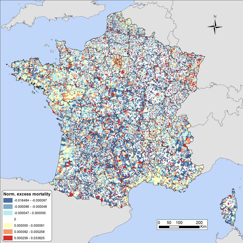
Figure 1: Normalized excess mortality in March 2020 in metropolitan France
Source: Authors’ elaboration on data from INSEE, fichier des décès, various releases, and INSEE, French
Population Census of 2016.
We need to introduce some simple notation to present the data on mortality: let mcity be
the number of deaths for individuals in the age group c, e.g., individuals aged 60 and above,
7in municipality i in the week t = 1, ..., 16 of the year y, with y = 2010, ..., 2020. We define
the weekly normalized excess mortality in 2020 as:
" 2019
#
1 1 X
ncit ≡ c mcit2020 − mc
si 10 y=2010 ity
where sci is the population in the age group c in municipality i according to the 2016 Popu-
lation Census. Thus, ncit gives us the excess mortality recorded in a given week of 2020 as a
share of the population at risk. Figure 1 reports the average normalized excess mortality for
each municipality in March 2020 for metropolitan France. The most severely affected areas,
notably the two regions of Grand-Est and Île de France, can be easily spotted in Figure 1,
but this map also reveals that there has been a substantial spatial heterogeneity in the initial
diffusion of the epidemics even across neighboring municipalities.
4 Econometric analysis
The dependent variable yitc of our econometric analysis is the inverse hyperbolic sine of the
group-specific normalized excess mortality ncit , with t = 1, ..., 16:
p
yitc = arcsinh (ncit ) = ln ncit c 2
+ 1 + (nit ) (1)
Two key properties of the inverse hyperbolic sine justify our choice concerning the trans-
formation of the dependent variable: first, arcsinh(x) is defined for any x ∈ R, and this
is a necessary feature as many French municipalities recorded a negative excess mortality
during the COVID-19 epidemics;24 second, arcsinh(x) is a contraction mapping on the whole
real line,25 and this feature contributes to reduce the weight of outlying observations in the
econometric analysis (Burbidge et al., 1988).
We bring to the data the following specification for a given age group c:
yitc = αtc ln (turnouti2020 )+βtc ln (turnouti2014 )+γ c0 xi +ddept(i) ×dt +cit , with t = 1, ..., 16, (2)
where turnouti2020 is the turnout in the first round of the municipal elections on March 15,
24
Bhalotra et al. (2017) also rely on the inverse
√ hyperbolic sine transformation of local mortality figures.
25
Notice that, ∀x ∈ R: ∂arcsinh(x)/∂x = 1/ 1 + x2 ≤ 1.
82020, which we assume to capture the extent of social interactions both on the day of the vote,
and in the electoral meetings in the previous weeks. The coefficient of this variable is week-
specific, in order to leave the time profile of the strength of the association between yitc and
turnouti2020 unrestricted. We also control for the (logarithm of) turnouti2014 , i.e., the turnout
rate in the first round of the previous municipal elections. In the baseline specification, the
vector of controls xi includes the logarithm of population density, but additional controls
are added in robustness checks that are described below. We also include interactive fixed
effects between the dummies for the department of each municipality and weekly dummies,
i.e., ddept(i) × dt , to allow for a flexible temporal evolution of excess mortality during the
epidemics in each French department.
A key concern relates to the endogeneity of ln (turnouti2020 ), as the turnout was probably
lower in municipalities that had been more severely affected already in the early stages
of the COVID-19 epidemics in France. We deal with the threat to identification due to
reverse causality by instrumenting ln (turnouti2020 ) with a measure of the intensity of electoral
competition in municipality i. In particular, we define zi2020 as the logarithm of the ratio
between the number of candidates, and the number of local councilors that had to be elected.
A higher value of zi2020 should have increased voter turnout, as it increased the stakes related
to the vote. A possible threat to the validity of our instrument is related to the fact that
the intensity of electoral competition within a department could be correlated with some
time-invariant characteristics of a municipality,26 such as the frequency of social interactions
or economic conditions, that could have exerted a direct effect on the level of mortality
registered over our period of analysis. We deal with this concern by including in Eq. (2) the
voter turnout in 2014, whose coefficient βtc is also allowed to vary with the week t = 1, ..., 16
of 2020, to capture the time-varying dependency between unobservables and excess mortality
as the epidemics unfolded.
26
The inclusion of interactive fixed effects between the dummies for the department of each municipality
and weekly dummies in Eq. (2) fully absorbs the variability across departments.
9Table 1: Econometric results (January 1st to April 21, 2020)
Dependent variable: inverse hyperbolic sine of
weekly normalized excess mortality
(1) (2) (3) (4) (5) (6)
OLS 2SLS OLS 2SLS OLS 2SLS
Age group c 60+ 60+ 70+ 70+ 80+ 80+
ln(turnout) × Mar. 18-24 -0.0000 0.0003∗∗∗ -0.0001 0.0004∗∗ -0.0001 0.0006
(0.0001) (0.0001) (0.0001) (0.0002) (0.0002) (0.0004)
ln(turnout) × Mar. 25-31 -0.0001∗∗ 0.0004∗∗∗ -0.0002∗∗ 0.0007∗∗∗ -0.0003∗ 0.0010∗
(0.0000) (0.0001) (0.0001) (0.0002) (0.0002) (0.0005)
ln(turnout) × Apr. 1-7 -0.0001∗ 0.0003∗∗ -0.0001 0.0005∗∗ -0.0003 0.0014∗∗∗
(0.0001) (0.0001) (0.0001) (0.0002) (0.0002) (0.0005)
ln(turnout) × Apr. 8-14 -0.0001∗∗ 0.0002 -0.0002∗∗ 0.0003 -0.0004∗∗ 0.0007∗
(0.0001) (0.0001) (0.0001) (0.0002) (0.0002) (0.0004)
ln(turnout) × Apr. 15-21 -0.0000 0.0003∗∗∗ -0.0000 0.0006∗∗∗ 0.0001 0.0012∗∗∗
(0.0000) (0.0001) (0.0001) (0.0002) (0.0002) (0.0004)
Observations 538,256 538,256 537,984 537,984 535,200 535,200
Under-ident. (p-value) 0.00 0.00 0.00
Kleinbergen-Paap F -test 39.22 39.60 39.86
First stage
Intensity of competition 0.2851∗∗∗ 0.2852∗∗∗ 0.2855∗∗∗
(0.0077) (0.0077) (0.0077)
Observations 538,256 537,984 535,200
R2 0.68 0.68 0.68
Notes: ***, **, and * denote significance at the 1, 5, and 10 percent levels, respectively; clustered standard
errors at the department level are reported in parentheses; all specifications also include interactions between
the turnout in 2020 and in 2014 and weekly dummies (coefficients not shown) for the 16 weeks included in
the analysis, the logarithm of population density, and department-week dummies; OLS and 2SLS regressions
have been estimated using the Stata commands reghdfe and ivreghdfe.
Source: Authors’ elaboration on data from INSEE (fichier des décès, 2016 Population Census), the Ministry
of Interior Affairs (electoral results for the first round of the municipal elections in 2014 and 2020), and
Open Street Map.
Table 1 reports the weekly coefficients for the municipal-level voter turnout in 2020 for
the five weeks after the election on March 15 obtained from the estimation of Eq. (2) with
OLS and 2SLS estimators for three nested age groups.27,28 Columns (1) and (2) focus on the
27
The sample sizes display minor differences when moving to older age groups as a few small-sized French
municipalities do not have, according to the 2016 Population Census, any resident aged above 70 or 80.
28
The five weeks between March 18 and April 21, 2020 broadly coincide with the period
10population aged 60 and above: when we instrument the endogenous turnout, we obtain a
positive and significant coefficient for four out of the five weeks after the municipal election,
showing that a higher turnout has resulted in a larger normalized excess mortality, while
OLS estimates are severely downward biased. The significance of the coefficient for March
18 to 24, i.e., just a few days after the election, strongly suggest that a part of the influence
on excess mortality is due to the electoral meetings that were held in the weeks right before
the first round. The Kleinbergen-Paap F -test is reassuring with respect to the strength of
our instrument. Coefficients are larger in magnitude, albeit less precisely estimated due to
the smaller size of the population at risk, when we focus on older age groups in the remaining
four data columns of Table 1.
Figure 2: Estimated weekly coefficients with 2SLS for the age group 60+
bt60+
α
0.0005
0
Week t
−0.0005
Jan. 1-7
Jan. 8-14
Jan. 15-21
Jan. 22-28
Jan. 29-Feb. 4
Feb. 5-11
Feb. 12-18
Feb. 19-25
Feb. 26-Mar. 3
Mar. 4-10
Mar. 11-17
Mar. 18-24
Mar. 25-31
Apr.1-7
Apr.8-14
Apr.15-21
Notes: estimated coefficients and 95 percent confidence intervals for the logarithm of the participation rate
in 2020 from the 2SLS estimation in Table 1 for the age group 60+.
btc for the first 16 weeks of 2020 from the 2SLS
Figure 2 reports the estimated coefficients α
specification in Table 1 for the population aged 60 and above. While the effect is positive
in which France experienced a positive excess mortality compared to previous years; by the
end of April, the daily country-level number of deaths had returned in line with the values
of previous years (see Table A.1 in the Appendix and also https://www.lemonde.fr/les-
decodeurs/article/2020/05/22/coronavirus-age-sexe-departement-la-hausse-de-
la-mortalite-francaise-en-sept-graphiques_6040465_4355770.html, last accessed on
June 5, 2020).
11and significant at the 5 percent confidence level in four out of the five weeks since March
15, 2020, the coefficient is never positive and significant at conventional confidence levels in
earlier weeks, and these placebos are reassuring with respect to the validity of our instrument.
btc for the first 16 weeks of 2020 from the
Similarly, Figure 3 plots the estimated coefficients α
same 2SLS specification as in Table 1, when this is estimated on the population aged 18 to
59. None of these weekly coefficients are significant, suggesting that the decision to maintain
the first round of the municipal elections increased mortality only for the elderly population.
Figure 3: Estimated weekly coefficients with 2SLS for the age group 18 to 59
bt18−59
α
0.0002
0
Week t
−0.0002
Jan. 1-7
Jan. 8-14
Jan. 15-21
Jan. 22-28
Jan. 29-Feb. 4
Feb. 5-11
Feb. 12-18
Feb. 19-25
Feb. 26-Mar. 3
Mar. 4-10
Mar. 11-17
Mar. 18-24
Mar. 25-31
Apr.1-7
Apr.8-14
Apr.15-21
Notes: estimated coefficients and 95 percent confidence intervals for the logarithm of the turnout in 2020
from a 2SLS for the age group 18 to 59 using the same specification as in Table 1.
We use the results from Table 1 from March 18 to April 21 to quantify the effects of
turnout on mortality for the municipalities in our sample. More precisely, we predict the
value of the dependent variable ybitc when (i) we replace ln (turnouti2020 ) with ln (turnouti2014 ),
or when (ii ) we add one standard deviation (equal to 14.5 percentage points) to the actual
turnout in 2020. We then invert ybitc for each of the five weeks,29 multiply it by the population
at risk sci and then sum over the five weeks and across all municipalities in our sample for
the population aged 60+, 70+ and 80+ to get the predicted increase in the total number of
deaths. Table 2 shows that the two counterfactual scenarios with a higher turnout correspond
to a death toll that is 4,135 and 5,335 higher than it is actually observed in the data for the
29
If y = arcsinh(x), then x = sinh(y) = [ey − e−y ] /2.
12population aged 60 and above. These two figures represent respectively 16.9 and 21.8 percent
of the observed total number of deaths over this five-week period. Table 2 also reveals that
the increase in the number of deaths is largely concentrated in the most vulnerable parts
of the population, as around 78 percent, i.e., 4, 152/5, 335 = 0.778, of the additional deaths
in the second counterfactual scenario relate to the individuals aged 80 and above. As our
sample selection criteria imply that we do not include in the analysis deaths occurring in
hospitals, these figures represent a lower-bound of the total absolute effect. This entails
that the historically unprecedented high level abstention has contributed to a significant
and sizable reduction in the number of deaths that would have been otherwise recorded in
France, thus lowering the cost in terms of human lives of the decision to maintain the first
round of the municipal elections.
Table 2: Additional deaths from March 18 to April 21, 2020 in two counterfactual scenarios
Age group c
All 60+ 70+ 80+
Average total deaths 2010-2019 17,125 15,199 13,461 11,021
Total deaths 2020 26,191 24,445 22,336 18,624
Difference 2020 vs. 2010-2019 9,066 9,246 8,875 7,603
Additional deaths
First scenario 4,135 3,715 3,224
Second scenario 5,335 4,795 4,152
Number of municipalities 33,694 33,641 33,624 33,450
Notes: in the first counterfactual scenario we increase the turnout in 2020 by one standard
deviation (14.5 percentage points), while in the second scenario we replace the turnout in 2020
with its municipal-specific 2014 value.
Source: Authors’ elaboration on data from INSEE, fichier des décès, electoral data for the
first-round of the municipal elections in 2014 and 2020 from the the Ministry of Interior Affairs,
and from the 2SLS estimates in the even data columns in Table 1.
The empirical evidence that we have presented is robust to the adoption of several alter-
native specifications or sample selection criteria, as shown in the Appendix Tables A.2-A.5:
(i ) estimating the model on the entire set of municipalities in metropolitan France; (ii )
dropping the departments with an early exposure to the COVID-19 epidemics, for which
the number of candidates might have been affected by the deteriorating health situation;
controlling (iii ) for the average turnout in 2020 in neighboring municipalities (within a 10
13km radius), and (iv ) for the shares of the population in each municipality in different age
cohorts,as individuals in different age groups might have adhered to a varying degree to the
recommended social-distancing measures. For (iii ) and (iv ), we also allow the coefficients of
these additional controls to vary at the weekly level, as we do for the voter turnout in 2014
and 2020.
5 Concluding remarks
We exploit the substantial spatial variation in voter turnout across municipalities, instru-
menting it with exogenous shifts in the local intensity of the electoral competition, to identify
its effect on the municipal-level excess mortality in the weeks after the election on March
15, 2020. The historically unprecedented level of abstention has contributed to mitigate the
effect produced by the controversial political decision to maintain the elections, which were
mostly felt by the population aged 80 and above. European governments should be cautious
about maintaining local or national elections in the coming months in case the COVID-19
epidemics were to regain momentum.
References
Bhalotra, S. R., A. Diaz-Cayeros, G. Miller, A. Miranda, and A. S.
Venkataramani (2017): “Urban Water Disinfection and Mortality Decline in Developing
Countries,” NBER Working Paper No. 23239, National Bureau of Economic Research.
Burbidge, J. B., L. Magee, and A. L. Robb (1988): “Alternative Transformations to
Handle Extreme Values of the Dependent Variable,” Journal of the American Statistical
Association, 83, 123–127.
Cassette, A., E. Farvaque, and J. Hericourt (2013): “Two-round elections, one-
round determinants? Evidence from the French municipal elections,” Public Choice, 156,
563–591.
Deschênes, O. and E. Moretti (2009): “Extreme Weather Events, Mortality, and Mi-
gration,” The Review of Economics and Statistics, 91, 659–681.
14Moatti, J.-P. (2020): “The French response to COVID-19: intrinsic difficulties at the
interface of science, public health, and policy,” The Lancet Public Health, 5, article e255.
Zeitoun, J.-D., M. Faron, S. Manternach, J. Fourquet, M. Lavielle, and
J. Lefevre (2020): “Reciprocal association between participation to a national election
and the epidemic spread of COVID-19 in France: nationwide observational and dynamic
modeling study.” MedRxiv, https://www.medrxiv.org/content/early/2020/
05/19/2020.05.14.20090100.
15A Appendix
A.1 Structure of the data from INSEE, fichier des décès
Table A.1: Weekly number of deaths in 2020 by month of release
February February February February
Month of release of the data
May April March February Total
Jan. 1-7 19 48 240 13,039 13,346
Jan. 8-14 22 51 335 12,889 13,307
Jan. 15-21 30 86 1,358 11,306 12,780
Jan. 22-28 34 90 3,313 9,319 12,765
Jan. 29-Feb. 4 57 157 11,896 781 12,891
Feb. 5-11 61 204 12,305 0 12,570
Feb. 12-18 95 569 11,913 0 12,577
Feb. 19-25 112 2,390 9,420 0 11,922
Feb. 26-Mar. 3 164 10,423 1,808 0 12,395
Mar. 4-10 325 12,138 0 0 12,463
Mar. 11-17 820 12,167 0 0 12,987
Mar. 18-24 1,843 12,377 0 0 14,220
Mar. 25-31 10,924 6,222 0 0 17,146
Apr. 1-7 18,592 0 0 0 18,592
Apr. 8-14 16,415 0 0 0 16,415
Apr. 15-21 13,492 0 0 0 13,492
Apr. 22-28 7,697 0 0 0 7,697
Apr. 29-May 5 59 0 0 0 59
Total 70,761 56,922 52,588 47,344 227,615
Notes: the data refer to all 33,694 municipalities in metropolitan France.
Source: Authors’ elaboration on INSEE, fichier des décès, February to May 2020
releases of the data.
16A.2 Additional results
Table A.2: Results on the full sample
Dependent variable: inverse hyperbolic sine of
weekly normalized excess mortality
(1) (2) (3) (4) (5) (6)
OLS 2SLS OLS 2SLS OLS 2SLS
Age group c 60+ 60+ 70+ 70+ 80+ 80+
ln(turnout) × Mar. 18-24 -0.0000 0.0004∗∗∗ -0.0001 0.0006∗∗ -0.0001 0.0007
(0.0001) (0.0001) (0.0001) (0.0002) (0.0003) (0.0005)
ln(turnout) × Mar. 25-31 -0.0001 0.0007∗∗∗ -0.0002 0.0013∗∗∗ -0.0003 0.0017∗∗
(0.0001) (0.0002) (0.0001) (0.0003) (0.0003) (0.0007)
ln(turnout) × Apr. 1-7 -0.0001 0.0007∗∗∗ -0.0001 0.0011∗∗∗ -0.0003 0.0024∗∗∗
(0.0001) (0.0002) (0.0002) (0.0003) (0.0003) (0.0006)
ln(turnout) × Apr. 8-14 -0.0001∗∗ 0.0005∗∗∗ -0.0002∗∗ 0.0008∗∗∗ -0.0005∗ 0.0016∗∗∗
(0.0001) (0.0001) (0.0001) (0.0002) (0.0002) (0.0005)
ln(turnout) × Apr. 15-21 0.0000 0.0006∗∗∗ 0.0001 0.0010∗∗∗ 0.0003 0.0021∗∗∗
(0.0001) (0.0001) (0.0001) (0.0002) (0.0002) (0.0005)
Observations 555,104 555,104 554,832 554,832 552,048 552,048
Under-ident. (p-value) 0.00 0.00 0.00
Kleinbergen-Paap F -test 34.46 34.76 35.19
Department-week FE Yes Yes Yes Yes Yes Yes
First stage
Intensity of competition 0.2619∗∗∗ 0.2620∗∗∗ 0.2624∗∗∗
(0.0072) (0.0072) (0.0072)
Observations 555,104 554,832 552,048
R2 0.68 0.68 0.68
Notes: ***, **, and * denote significance at the 1, 5, and 10 percent levels, respectively; clustered standard
errors at the department level are reported in parentheses; all specifications also include interactions between
the turnout in 2020 and in 2014 and weekly dummies (coefficients not shown) for the 16 weeks included
in the analysis, and the logarithm of population density; OLS and 2SLS regressions have been estimated
using the Stata commands reghdfe and ivreghdfe.
Source: Authors’ elaboration on data from INSEE (fichier des décès, 2016 Population Census), the Ministry
of Interior Affairs, and Open Street Map.
17Table A.3: Results when dropping early exposed departments
Dependent variable: inverse hyperbolic sine of
weekly normalized excess mortality
(1) (2) (3) (4) (5) (6)
OLS 2SLS OLS 2SLS OLS 2SLS
Age group c 60+ 60+ 70+ 70+ 80+ 80+
ln(turnout) × Mar. 18-24 -0.0000 0.0003∗∗∗ -0.0000 0.0005∗∗ -0.0000 0.0005
(0.0001) (0.0001) (0.0001) (0.0002) (0.0002) (0.0004)
ln(turnout) × Mar. 25-31 -0.0001∗ 0.0003∗∗ -0.0002 0.0005∗∗ -0.0002 0.0008
(0.0001) (0.0001) (0.0001) (0.0002) (0.0002) (0.0005)
ln(turnout) × Apr. 1-7 -0.0001 0.0004∗∗∗ -0.0000 0.0005∗∗ -0.0002 0.0017∗∗∗
(0.0001) (0.0001) (0.0001) (0.0002) (0.0002) (0.0005)
ln(turnout) × Apr. 8-14 -0.0001∗∗∗ 0.0001 -0.0003∗∗∗ 0.0001 -0.0005∗∗ 0.0003
(0.0001) (0.0001) (0.0001) (0.0002) (0.0002) (0.0005)
ln(turnout) × Apr. 15-21 -0.0001 0.0003∗∗ -0.0001 0.0005∗∗∗ -0.0001 0.0008∗∗
(0.0000) (0.0001) (0.0001) (0.0002) (0.0002) (0.0004)
Observations 478,752 478,752 478,496 478,496 476,000 476,000
Under-ident. (p-value) 0.00 0.00 0.00
Kleinbergen-Paap F -test 41.12 41.65 41.55
Department-week FE Yes Yes Yes Yes Yes Yes
First stage
Intensity of competition 0.2759∗∗∗ 0.2759∗∗∗ 0.2763∗∗∗
(0.0071) (0.0071) (0.0071)
Observations 478,752 478,496 476,000
R2 0.67 0.67 0.67
Notes: ***, **, and * denote significance at the 1, 5, and 10 percent levels, respectively; clustered standard
errors at the department level are reported in parentheses; all specifications also include interactions between
the turnout in 2020 and in 2014 and weekly dummies (coefficients not shown) for the 16 weeks included in
the analysis, and the logarithm of population density; the sample excludes municipalities in all departments
with more than 50 COVID-19 deaths by the end of March according to Santé publique France (Bas-Rhin,
Haut-Rhin, Hauts-de-Seine, Moselle, Oise, Paris, Rhône, Seine-Saint-Denis, Val-de-Marne, Val-d’Oise, Vosges,
Yvelines), and Haute-Savoie, which registered one of the first major clusters of cases; OLS and 2SLS regressions
have been estimated using the Stata commands reghdfe and ivreghdfe.
Source: Authors’ elaboration on data from INSEE (fichier des décès, 2016 Population Census), the Ministry
of Interior Affairs, and Open Street Map.
18Table A.4: Results with the average 2020 turnout in neighboring municipalities
Dependent variable: inverse hyperbolic sine of
weekly normalized excess mortality
(1) (2) (3) (4) (5) (6)
OLS 2SLS OLS 2SLS OLS 2SLS
Age group c 60+ 60+ 70+ 70+ 80+ 80+
ln(turnout) × Mar. 18-24 -0.0000 0.0002∗∗∗ -0.0001 0.0004∗∗ -0.0001 0.0006∗
(0.0001) (0.0001) (0.0001) (0.0002) (0.0002) (0.0003)
ln(turnout) × Mar. 25-31 -0.0001∗∗ 0.0003∗∗∗ -0.0002∗ 0.0005∗∗∗ -0.0002 0.0008∗
(0.0000) (0.0001) (0.0001) (0.0002) (0.0002) (0.0004)
ln(turnout) × Apr. 1-7 -0.0001∗ 0.0003∗∗ -0.0001 0.0004∗∗ -0.0003 0.0012∗∗
(0.0001) (0.0001) (0.0001) (0.0002) (0.0002) (0.0005)
ln(turnout) × Apr. 8-14 -0.0001∗∗∗ 0.0001 -0.0003∗∗ 0.0003∗ -0.0005∗∗ 0.0007∗
(0.0001) (0.0001) (0.0001) (0.0002) (0.0002) (0.0004)
ln(turnout) × Apr. 15-21 0.0000 0.0002∗∗∗ 0.0000 0.0005∗∗∗ 0.0002 0.0010∗∗∗
(0.0000) (0.0001) (0.0001) (0.0001) (0.0002) (0.0003)
Observations 538,256 538,256 537,984 537,984 535,200 535,200
Under-ident. (p-value) 0.00 0.00 0.00
Kleinbergen-Paap F -test 84.00 84.28 84.60
Department-week FE Yes Yes Yes Yes Yes Yes
First stage
Intensity of competition 0.2846∗∗∗ 0.2846∗∗∗ 0.2850∗∗∗
(0.0073) (0.0073) (0.0073)
Observations 538,256 537,984 535,200
R2 0.69 0.69 0.69
Notes: ***, **, and * denote significance at the 1, 5, and 10 percent levels, respectively; clustered standard
errors at the department level are reported in parentheses; all specifications also include the turnout in 2020,
in 2014, and the average turnout in 2020 in the municipalities within a 10 km radius (week-specific coefficients
not shown), and the logarithm of population density; OLS and 2SLS regressions have been estimated using
the Stata commands reghdfe and ivreghdfe.
Source: Authors’ elaboration on data from INSEE (fichier des décès, 2016 Population Census), the Ministry
of Interior Affairs, and Open Street Map.
19Table A.5: Results with shares of population in different age groups
Dependent variable: inverse hyperbolic sine of
weekly normalized excess mortality
(1) (2) (3) (4) (5) (6)
OLS 2SLS OLS 2SLS OLS 2SLS
Age group c 60+ 60+ 70+ 70+ 80+ 80+
ln(turnout) × Mar. 18-24 -0.0000 0.0002∗∗ -0.0001 0.0003∗ -0.0001 0.0004
(0.0001) (0.0001) (0.0001) (0.0002) (0.0002) (0.0004)
ln(turnout) × Mar. 25-31 -0.0001∗∗ 0.0003∗∗∗ -0.0002∗∗ 0.0006∗∗∗ -0.0003∗∗ 0.0009
(0.0001) (0.0001) (0.0001) (0.0002) (0.0002) (0.0006)
ln(turnout) × Apr. 1-7 -0.0001∗∗ 0.0002 -0.0001 0.0003 -0.0004 0.0011∗∗
(0.0001) (0.0001) (0.0001) (0.0002) (0.0002) (0.0005)
ln(turnout) × Apr. 8-14 -0.0001∗∗∗ 0.0001 -0.0002∗∗ 0.0002 -0.0005∗∗ 0.0006
(0.0001) (0.0001) (0.0001) (0.0002) (0.0002) (0.0004)
ln(turnout) × Apr. 15-21 -0.0000 0.0002∗∗∗ -0.0000 0.0004∗∗∗ 0.0001 0.0010∗∗
(0.0000) (0.0001) (0.0001) (0.0002) (0.0002) (0.0004)
Observations 538,256 538,256 537,984 537,984 535,200 535,200
Under-ident. (p-value) 0.00 0.00 0.00
Kleinbergen-Paap F -test 42.43 42.76 42.92
Department-week FE Yes Yes Yes Yes Yes Yes
First stage
Intensity of competition 0.2859∗∗∗ 0.2860∗∗∗ 0.2863∗∗∗
(0.0078) (0.0078) (0.0078)
Observations 538,256 537,984 535,200
R2 0.68 0.68 0.68
Notes: ***, **, and * denote significance at the 1, 5, and 10 percent levels, respectively; clustered standard
errors at the department level are reported in parentheses; all specifications also include the turnout in 2020,
in 2014, and share of the population in the 18-39, 40-59, 60-69, 70-79 and 80 and above (0-17 is the omitted
category), age groups (week-specific coefficients not shown), and the logarithm of population density; OLS
and 2SLS regressions have been estimated using the Stata commands reghdfe and ivreghdfe.
Source: Authors’ elaboration on data from INSEE (fichier des décès, 2016 Population Census), the Ministry
of Interior Affairs, and Open Street Map.
20You can also read