UNCERTAINTY IN NEURAL PROCESSES - OpenReview
←
→
Page content transcription
If your browser does not render page correctly, please read the page content below
Under review as a conference paper at ICLR 2021

U NCERTAINTY IN N EURAL P ROCESSES
 Anonymous authors
 Paper under double-blind review

                                             A BSTRACT
         We explore the effects of architecture and training objective choice on amortized
         posterior predictive inference in probabilistic conditional generative models. We
         aim this work to be a counterpoint to a recent trend in the literature that stresses
         achieving good samples when the amount of conditioning data is large. We instead
         focus our attention on the case where the amount of conditioning data is small. We
         highlight specific architecture and objective choices that we find lead to qualita-
         tive and quantitative improvement to posterior inference in this low data regime.
         Specifically we explore the effects of choices of pooling operator and variational
         family on posterior quality in neural processes. Superior posterior predictive sam-
         ples drawn from our novel neural process architectures are demonstrated via image
         completion/in-painting experiments.

1   I NTRODUCTION
What makes a probabilistic conditional generative model good? The belief that a generative model
is good if it produces samples that are indistinguishable from those that it was trained on (Hinton,
2007) is widely accepted, and understandably so. This belief also applies when the generator is
conditional, though the standard becomes higher: conditional samples must be indistinguishable
from training samples for each value of the condition.
Consider an amortized image in-painting task in which the objective is to fill in missing pixel values
given a subset of observed pixel values. If the number and location of observed pixels is fixed, then
a good conditional generative model should produce sharp-looking sample images, all of which
should be compatible with the observed pixel values. If the number and location of observed pixels
is allowed to vary, the same should remain true for each set of observed pixels. Recent work on this
problem has focused on reconstructing an entire image from as small a conditioning set as possible.
As shown in Fig. 1, state-of-the-art methods (Kim et al., 2018) achieve high-quality reconstruction
from as few as 30 conditioning pixels in a 1024-pixel image.
Our work starts by questioning whether reconstructing an image from a small subset of pixels is
always the right objective. To illustrate, consider the image completion task on handwritten digits.
A small set of pixels might, depending on their locations, rule out the possibility that the full image
is, say, 1, 5, or 6. Human-like performance in this case would generate sharp-looking sample images
for all digits that are consistent with the observed pixels (i.e., 0, 2-4, and 7-9). Observing additional
pixels will rule out successively more digits until the only remaining uncertainty pertains to stylistic
details. The bottom-right panel of Fig. 1 demonstrates this type of “calibrated” uncertainty.
We argue that in addition to high-quality reconstruction based on large conditioning sets, amortized
conditional inference methods should aim for meaningful, calibrated uncertainty, particularly for
small conditioning sets. For different problems, this may mean different things (see discussion in
Section 3). In this work, we focus on the image in-painting problem, and define well calibrated
uncertainty to be a combination of two qualities: high sample diversity for small conditioning sets;
and sharp-looking, realistic images for any size of conditioning set. As the size of the conditioning
set grows, we expect the sample diversity to decrease and the quality of the images to increase.
We note that this emphasis is different from the current trend in the literature, which has focused
primarily on making sharp and accurate image completions when the size of the conditioning context
is large (Kim et al., 2018).
To better understand and make progress toward our aim, we employ posterior predictive inference
in a conditional generative latent-variable model, with a particular focus on neural processes (NPs)

                                                   1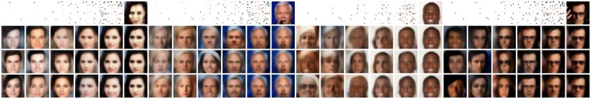
Under review as a conference paper at ICLR 2021
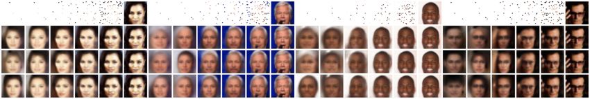
Figure 1: Representative image in-painting results for CelebA and MNIST. From left to right, neural
process (NP) (Garnelo et al., 2018b), attentive neural process (ANP) (Kim et al., 2018), and ours.
Top rows show context sets of given pixels, ranging from very few pixels to all pixels. In each
panel the ground truth image (all pixels) is in the upper right corner. The rows correspond to i.i.d.
samples from the corresponding image completion model given only the pixels shown in the top row
of the same column. Our neural process with semi-implicit variational inference and max pooling
produces results with the following characteristics: 1) the images generated with a small amount of
contextual information are “sharper” and more face- and digit-like than NP results and 2) there is
greater sample diversity across the i.i.d. samples than those from the ANP. This kind of “calibrated
uncertainty” is what we target throughout.
(Garnelo et al., 2018a;b). We find that particular architecture choices can result in markedly different
performance. In order to understand this, we investigate posterior uncertainty in NP models (Sec-
tion 4), and we use our findings to establish new best practices for NP amortized inference artifacts
with well-calibrated uncertainty. In particular, we demonstrate improvements arising from a com-
bination of max pooling, a mixture variational distribution, and a “normal” amortized variational
inference objective.
The rest of this paper is organized as follows. Section 2 and Section 3 present background material
on amortized inference for generative models and calibrated uncertainty, respectively. Section 4
discusses and presents empirical evidence for how NP models handle uncertainty. Section 5 intro-
duces our proposed network architecture and objective. Section 6 reports our results on the MNIST,
FashionMNIST and CelebA datasets. Finally, Section 7 presents our conclusions.
2 A MORTIZED I NFERENCE FOR C ONDITIONAL G ENERATIVE M ODELS
Our work builds on amortized inference (Gershman & Goodman, 2014; Kingma & Welling, 2014),
probabilistic meta-learning (Gordon et al., 2019), and conditional generative models in the form of
neural processes (Garnelo et al., 2018b; Kim et al., 2018). This section provides background.
Let (xC , yC ) = {(xi , yi )}ni=1 and (xT , yT ) = {(x0j , yj0 )}m
j=1 be a context set and target set respec-
tively. In image in-painting, the context set input xC is a subset of an image’s pixel coordinates, the
context set output yC are the corresponding pixel values (greyscale intensity or colors), the target
set input xT is a set of pixel coordinates requiring in-painting, and the target set output yT is the
corresponding set of target pixel values. The corresponding graphical model is shown in Fig. 2.
The goal of amortized conditional inference is to rapidly approximate, at “test time,” the posterior
predictive distribution
Z
pθ (yT |xT , xC , yC ) = pθ (yT |xT , z)pθ (z|xC , yC )dz . (1)
2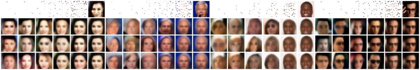
Under review as a conference paper at ICLR 2021

Figure 2: Generative graphical model for a single neural process task. C is the task “context” set of
input/output pairs (xi , yi ) and T is a target set in which only the input values are known.

We can think of the latent variable z as representing a problem-specific task-encoding. The like-
lihood term pθ (yT |xT , z) shows that the encoding parameterizes a regression model linking the
target inputs to the target outputs. In the NP perspective, z is a function and Eq. (1) can be seen as
integrating over the regression function itself, as in Gaussian process regression (Rasmussen, 2003).
Variational inference There are two fundamental aims for amortized inference for conditional
generative models: learning the model, parameterized by θ, that produces good samples, and pro-
ducing an amortization artifact, parameterized by φ, that can be used to approximately solve Eq. (1)
quickly at test time. Variational inference techniques couple the two learning problems. Let y and
x be task-specific output and input sets, respectively, and assume that at training time we know the
values of y. We can construct the usual single-training-task evidence lower bound (ELBO) as
                                                        h                     i
                          log pθ (y|x) ≥ Ez∼qφ (z|x,y) log pθ (y|z,x)p  θ (z)
                                                               qφ (z|x,y)       .                (2)
Summing over all training examples and optimizing Eq. (2) with respect to φ learns an amortized
inference artifact that takes a context set and returns a task embedding; optimizing with respect to θ
learns a problem-specific generative model. Optimizing both simultaneously results in an amortized
inference artifact bespoke to the overall problem domain.
At test time the learned model and inference artifacts can be combined to perform amortized poste-
rior predictive inference, approximating Eq. (1) with
                                               Z
                       pθ (yT |xT , xC , yC ) ≈ pθ (yT |xT , z)qφ (z|xC , yC )dz .             (3)

Crucially, given an input (xC , yC ), sampling from this distribution is as simple as sampling a
task embedding z from qφ (z|xC , yC ) and then passing the sampled z to the generative model
pθ (yT |xT , z) to produce samples from the conditional generative model.
Meta-learning The task-specific problem becomes a meta-learning problem when learning a re-
gression model θ that performs well on multiple tasks with the same graphical structure, trained
on data for which the target outputs {yj0 } are observed as well. In training our in-painting models,
following conventions in the literature (Garnelo et al., 2018a;b), tasks are simply random-size sub-
sets of random pixel locations x and values y from training set images. This random subsetting of
training images into context and target sets transforms this into a meta-learning problem, and the
“encoder” qφ (z|x, y) must learn to generalize over different context set sizes, with less posterior
uncertainty as the context set size grows.
Neural processes Our work builds on neural processes (NPs) (Garnelo et al., 2018a;b). NPs are
deep neural network conditional generative models. Multiple variants of NPs have been proposed
(Garnelo et al., 2018a;b; Kim et al., 2018), and careful empirical comparisons between them appear
in the literature (Grover et al., 2019; Le et al., 2018).
NPs employ an alternative training objective to Eq. (2) arising from the fact that the graphical model
in Fig. 2 allows a Bayesian update on the distribution of z, conditioning on the entire context set to
produce a posterior pθ (z|xC , yC ). If the generative model is in a tractable family that allows analytic
updates of this kind, then the NP objective corresponds to maximizing
                   h                                   i                    h                              i
                                                                                p (y |z,xT )qφ (z|xC ,yC )
  Ez∼qφ (z|xT ,yT ) log pθ (yT q|z,x T )pθ (z|xC ,yC )
                                 φ (z|xT ,yT )
                                                         ≈ Ez∼qφ (z|xT ,yT ) log θ T qφ (z|x T ,yT )
                                                                                                             (4)
where replacing pθ (z|xC , yC ) with its variational approximation is typically necessary because most
deep neural generative models have a computationally inaccessible posterior. This “NP objective”

                                                       3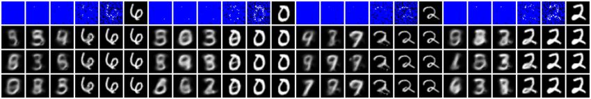
Under review as a conference paper at ICLR 2021

                     −410                                                                            1000

                                                                             Classifier prediction
    H(qφ (z|xC , yC ))
                                                                                                      800
                     −420

                                                                                                      600
                     −430
                                                                                                      400
                     −440
                                                                                                      200
                     −450
                                                                                                        0
                                   200     400    600       800   1000                                        200     400     600       800   1000
                                         Context set size                                                           Context set size

                            (a) Variational posterior entropy                                               (b) Classifier prediction

Figure 3: Posterior contraction of qφ (z|xC , yC ) in a NP+max pooling model. (a) The entropy of
qφ (z|xC , yC ) as a function of context set size, averaged over different tasks (images) and context
sets. The gray shaded area in both plots indicates context set sizes that did not appear in the training
data for the amortization artifact. (b) Predictions of a classifier trained to infer the context set size
given only sC , the pooled embedding of a context set. Equivalent results for the standard NP+mean
pooling encoder and for ANP appear in the Supplementary Material.

can be trained end-to-end, optimizing for both φ and θ simultaneously, where the split of training
data into context and target sets must vary in terms of context set size. The choice of optimizing
Eq. (4) instead of Eq. (2) is largely empirical (Le et al., 2018).

3              C ALIBRATED U NCERTAINTY

Quantifying and calibrating uncertainty in generative models remains an open problem, particularly
in the context of amortized inference. Previous work on uncertainty calibration has focused on
problems with relatively simpler structure. For example, in classification and regression problems
with a single dataset, prior work framed the problem as predicting a cumulative distribution function
that is close to the data-generating distribution, first as a model diagnostic (Gneiting et al., 2007) and
subsequently as a post-hoc adjustment to a learned predictor (Kuleshov et al., 2018). A version of
the latter approach was also applied to structured prediction problems (Kuleshov & Liang, 2015).
Previous approaches are conceptually similar to our working definition of calibrated uncertainty.
However, we seek calibrated uncertainty on a per-image, per-conditioning set basis, which is fun-
damentally different from previous settings. Quantification of all aspects of generative model per-
formance is an area of ongoing research, with uncertainty quantification a particularly challenging
problem.

4              U NCERTAINTY IN N EURAL P ROCESS MODELS

In this section, we investigate how NP models handle uncertainty. A striking property of NP models
is that as the size of the (random) context set increases, there is less sampling variation in target
samples generated by passing z ∼ qφ (z|xC , yC ) through the decoder. The samples shown in Fig. 1
are the likelihood mean (hence a deterministic function of z), and so the reduced sampling variation
can only be produced by decreased posterior uncertainty. Our experiments confirm this, as shown in
Fig. 3a: posterior uncertainty (as measured by entropy) decreases for increasing context size, even
beyond the maximum training context size. Such posterior contraction is a well-studied property
of classical Bayesian inference and is a consequence of the inductive bias of exchangeable models.
However, NP models do not have the same inductive bias explicitly built in. How do trained NP
models exhibit posterior contraction without being explicitly designed to do so? How do they learn
to do so during training?
A simple hypothesis is that the network somehow transfers the context size through the pooling op-
eration and into ρφ (sC ), which uses that information to set the posterior uncertainty. That hypothesis
is supported by Fig. 3b, which shows the results of training a classifier to infer the context size given

                                                                         4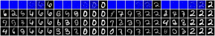
Under review as a conference paper at ICLR 2021

                                                                            −410                           greedy-entropy
                                                                                                           greedy-KL

                                                       H(qφ (z|xC , yC ))
       10                50               100                               −420                           random

                                                                            −430

                                                                            −440

                                                                            −450

                                                                                   0   50   100    150    200    250    300
                                                                                             Context set size

Figure 4:       (Left) The first {10, 50, 100} pixels greedily chosen to minimize
DKL (qφ (z|x, y)||qφ (z|xC , yC )). These pixels are highly informative about z, but only a
subset of them will appear in the vast majority of random context sets. (Right) Posterior entropy
decreasing as context size increases, for different methods of generating a context set: green is
the average over 100 random context sets of each size; blue greedily chooses context pixels to
minimize posterior entropy; and orange greedily minimizes DKL (qφ (z|x, y)||qφ (z|xC , yC )). The
black dashed line represents the posterior entropy when conditioned on the full image.

only sC . However, consider that within a randomly generated context set, some observations are
more informative than others. For example, Fig. 4 shows the first {10, 50, 100} pixels of an MNIST
digit 2, greedily chosen to minimize DKL (qφ (z|x, y)||qφ (z|xC , yC )). If z is interpreted to represent,
amongst other things, which digit the image contains, then a small subset of pixels determine which
digits are possible.
It is these highly informative pixels that drive posterior contraction in a trained NP. In a random con-
text set, the number of highly informative pixels is random. For example, a max-pooled embedding
saturates with the M most highly informative context pixels, where M ≤ d, the dimension of em-
bedding space. On average, a random context set of size n, taken from an image with N pixels, will
contain only nM/N of the informative pixels. In truth, Fig. 3 displays how the information content of
a context depends, on average, on the size of that context. Indeed, greedily choosing context pixels
results in much faster contraction (Fig. 4).
Learning to contract          Posterior contraction is implicitly encouraged by the NP objective Eq. (4).
It can be rewritten as
            Ez∼qφ (z|xT ,yT ) [log pθ (yT |z, xT )] − DKL (qφ (z|xT , yT )||qφ (z|xC , yC )) .                              (5)
The first term encourages perfect reconstruction of yT , and discourages large variations in z ∼
qφ (z|xT , yT ), which would result in large variations in predictive log-likelihood. This effect is
stronger for larger target sets since there are more target pixels to predict. In practice, C ⊂ T , so
the first term also (indirectly) encourages posterior contraction for increasing context sizes. The sec-
ond term, DKL (qφ (z|xT , yT )||qφ (z|xC , yC )), reinforces the contraction by encouraging the context
posterior to be close to the target posterior.
Although the objective encourages posterior contraction, the network mechanisms for achieving
contraction are not immediately clear. Ultimately, the details depend on interplay between the pixel
embedding function, hφ , the pooling operation ⊕, and ρφ . We focus on mean and max pooling.
Max pooling As the size of the context set increases, the max-pooled embedding sC = ⊕ni=1 si
is non-decreasing in n; in a trained NP model, ||sC || will increase each time an informative pixel
is added to the context set; it will continue increasing until the context embedding saturates at the
full image embedding. At a high level, this property of max-pooling means that the σC component
of ρφ (sC ) has a relatively simple task: represent a function such that the posterior entropy is a
decreasing function of all dimensions of the embedding space. An empirical demonstration that ρφ
achieves this can be found in the Supplementary Material.
Mean pooling For a fixed image, as the size of a random context set increases, its mean-pooled
embedding will, on average, become closer to the full image embedding. Moreover, the mean-
pooled embeddings of all possible context sets of the image are contained in the convex set whose

                                                      5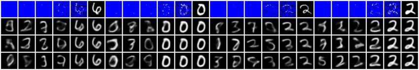
Under review as a conference paper at ICLR 2021

                         (a) encoder                                         (b) decoder

Figure 5: Our modified neural process architecture. The encoder produces a permutation invariant
embedding that parameterizes a stochastic task encoding z as follows: features extracted from each
element of the context set using neural net hφ are pooled, then passed to other neural networks ρφ
and ηφ that control the distribution over task embedding z. The decoder uses such a task encoding
along with embeddings of target inputs to produce the output distribution for each target input.

hull is formed by (a subset of) the individual pixel embeddings. The σC component of ρφ (sC ), then,
must approximate a function such that the posterior entropy is a convex function on the convex
set formed by individual pixel embeddings, with minimum at or near the full image embedding.
Learning such a function across the embeddings of many training images seems a much harder
learning task than that required by max pooling, which may explain the better performance of max
pooling relative to mean pooling in NPs (see Section 6).
Generalizing posterior contraction Remarkably, trained NP-based models generalize their pos-
terior contraction to context and target sizes not seen during training (see Fig. 3). The discussion
of posterior contraction in NPs using mean and max pooling in the previous paragraphs highlights
a shared property: for both models, the pooled embeddings of all possible context sets that can be
obtained from an image are in a convex set that is determined by a subset of possible context set
embeddings. For max-pooling, the convex set is formed by the max-pooled embedding of the M
“activation” pixels. For mean-pooling, the convex set is obtained from the convex hull of the indi-
vidual pixel embeddings. Furthermore, the full image embedding in both cases is contained in the
convex set. We conjecture that a sufficient condition for an NP image completion model to yield
posterior contraction that generalizes to context sets of unseen size is as follows: For any image,
the pooled embedding of every possible context set (which includes the full image) lies in a convex
subset of the embedding space.

5    N ETWORK ARCHITECTURE
The network architectures we employ for our experiments build on NPs, inspired by our findings
from Section 4. We describe them in detail in this section.
Encoder The encoder qφ (z|xC , yC ) takes input observations from an i.i.d. model (see Fig. 2, plate
over C), and therefore its encoding of those observations must be permutation invariant if it is to be
learned efficiently. Our qφ , as in related NP work, has a permutation-invariant architecture,
si = hφ (xi , yi ), 1 ≤ i ≤ n;   sC = ⊕ni=1 si ;   (µC , σC ) = ρφ (sC );   qφ (z|xC , yC ) = N (µC , σC2 ) .
Here ρφ and hφ are neural networks and ⊕ is a permutation-invariant pooling operator. Fig. 5
contains diagrams of a generalization of this encoder architecture (see below). The standard NP
architecture uses mean pooling; motivated by our findings in Section 4, we also employ max pooling.
Hierarchical Variational Inference In order to achieve better calibrated uncertainty in small con-
text size regimes, a more flexible approximate posterior could be beneficial. tConsider the MNIST
experiment shown in Fig. 6. Intuitively, an encoder could learn to map from the context set to a
one-dimensional discrete z value that lends support only to those digits that are compatible with
the context pixel values at the given context pixel locations (xC , yC ). This suggests that qφ should
be flexible enough to produce a multimodal distribution over z, which can be encouraged by mak-
ing qφ a mixture and corresponds to a hierarchical variational distribution (Ranganath et al., 2016;

                                                    6
Under review as a conference paper at ICLR 2021
1 2 3 5 10 15 30 90 150 300 1024 1 2 3 5 10 15 30 90 150 300 1024
Context
Context
Sample 3 Sample 2 Sample 1
Sample 3 Sample 2 Sample 1
std
std
0.00 0.05 0.10 0.15 0.20 0.25 0.0 0.1 0.2 0.3 0.4
(a) NP objective with mean pooling (b) NP objective with average pooling
1 2 3 5 10 15 30 90 150 300 1024 1 2 3 5 10 15 30 90 150 300 1024
Context
Context
Sample 3 Sample 2 Sample 1
Sample 3 Sample 2 Sample 1
std
std
0.00 0.05 0.10 0.15 0.20 0.25 0.00 0.05 0.10 0.15 0.20 0.25 0.30 0.35 0.40
(c) ANP (d) ANP
1 2 3 5 10 15 30 90 150 300 1024 1 2 3 5 10 15 30 90 150 300 1024
Context
Context
Sample 3 Sample 2 Sample 1
Sample 3 Sample 2 Sample 1
std
std
0.00 0.05 0.10 0.15 0.20 0.25 0.30 0.00 0.05 0.10 0.15 0.20 0.25 0.30
(e) NP+SIVI objective with max pooling (f) NP+SIVI objective with max pooling
Figure 6: Example MNIST and CelebA image completion tasks, for each of three NP methods. The
following guide applies to each block. The top row shows context sets of different sizes (context
sets are exactly the same for all methods), i.e., one task per column. The ground truth image is in the
upper right corner. The rows correspond to the mean function produced by gθ for different sampled
values of z. The bottom row shows an empirical estimate of the standard deviation of the mean
function from 1000 draws of z, a direct visualization of the uncertainty encoding.
Yin & Zhou, 2018; Sobolev & Vetrov, 2019). Specifically, the encoder structure described above,
augmented with a mixture variable is
Z
qφ (z|x, y) = qφ (ψ|x, y)qφ (z|ψ, x, y)dψ . (6)
This is shown in Fig. 5. For parameter-learning, the ELBO in Eq. (2) is targeted. However, the
hierarchical structure of the encoder makes this objective intractable. Therefore, a tractable lower
bound to the ELBO is used as the objective instead. In particular, the objective is based on semi-
implicit variational inference (SIVI) (See Appendix A.3).
Decoder The deep neural network stochastic decoder in our work is standard and not a focus. Like
other NP work, the data generating conditional likelihood
Qm in our decoder is assumed to factorize in
a conditionally independent way, pθ (yT |z, xT ) = i=1 pθ (yi0 |z, x0i ), where m is the size of the
target set and x0i and yi0 are a target set input and output respectively. Fig. 5b shows the decoder
architecture, with the neural network gθ the link function to a per pixel likelihood.
6 E XPERIMENTAL EVALUATION
We follow the experimental setup of Garnelo et al. (2018b), where images are interpreted as func-
tions that map pixel locations to color values, and image in-painting is framed as an amortized
7Under review as a conference paper at ICLR 2021
Method MNIST FashionMNIST CelebA
NP+mean 0.96 ± 0.12 0.93 ± 0.15 2.91 ± 0.30
ANP+mean 0.55 ± 0.12 0.57 ± 0.11 1.81 ± 0.18
NP+max 1.07 ± 0.11 1.02 ± 0.19 3.17 ± 0.30
SIVI+max 0.99 ± 0.25 0.96 ± 0.16 2.99 ± 0.39
Table 1: Predictive held-out test log-likelihood
NP+mean NP+max ANP SIVI+max
MNIST FashionMNIST CelebA
Inception score
10
7.5
4
5.0
5
2.5 2
100 101 102 103 100 101 102 103 100 101 102 103
Context set size Context set size Context set size
Figure 7: Inception scores of conditional samples.
predictive inference task where the latent image-specific regression function needs to be inferred
from a small context set of provided pixel values and locations. For ease of comparison to prior
work, we use the same MNIST (LeCun et al., 1998) and CelebA (Liu et al., 2015) datasets. Addi-
tionally, we run an experiment on FashionMNIST dataset (Xiao et al., 2017). Specific architecture
details for all networks are provided in Appendix A and open-source code for all experiments will
be released at the time of publication.
Qualitative Results Fig. 6 shows qualitative image in-painting results for MNIST and CelebA
images. Qualitative results for FashionMNIST are shown in Appendix D. It is apparent in all three
contexts that ANPs perform poorly when the context set is small, despite the superior sharpness of
their reconstructions when given large context sets. The sets of digits and faces that ANPs produce
are not sharp, realistic, nor diverse. On the other hand, their predecessor, NP (with mean pooling),
arguably exhibits more diversity but suffers at all context sizes in terms of realism of the images.
Our NP+SIVI with max pooling approach produces results with two important characteristics: 1) the
images generated with a small amount of contextual information are sharper and more realistic; and
2) there is high context-set-compatible variability across the i.i.d. samples. These qualitative results
demonstrate that max pooling plus the SIVI objective result in posterior mean functions that are
sharper and more appropriately diverse, except in the high context set size regime where diversity
does not matter and ANP produces much sharper images. Space limitations prohibit showing large
collections of samples where the qualitative differences are even more readily apparent. Appendix L
contains more comprehensive examples with greater numbers of samples.
Quantitative Results Quantitatively assessing posterior predictive calibration is an open prob-
lem (Salimans et al., 2016; Heusel et al., 2017). Table 1 reports, for the different architectures we
consider, predictive held out test-data log-likelihoods averaged over 10,000 MNIST, 10,000 Fash-
ionMNIST and 19,962 CelebA test images respectively. While the reported results make it clear that
max pooling improves held-out test likelihood, likelihood alone does not provide a direct measure
of sample quality nor diversity. It simply measures how much mass is put on each ground-truth
completion. It is also important to note that in our implementation of ANP, in contrast to its orig-
inal paper, the observation variance is fixed and that is why ANP performs poorly in Table 1. An
ANP model with learned observation variance outperforms all the other models in terms of held-out
test likelihood. However, it is empirically shown that learning the observation variance in NP mod-
els with a deterministic path (including ANPs) hurts the diversity of generated samples (Le et al.,
2018) (see Appendix C for a detailed discussion and additional results for ANP model with learned
variance).
Borrowing from the generative adversarial networks community, who have faced the similar prob-
lems of how to quantitatively evaluate models via examination of the samples they generate, we
8Under review as a conference paper at ICLR 2021
compute inception scores (Salimans et al., 2016) using conditionally generated samples for different
context set sizes for all of the considered NP architectures and report them in Fig. 7. Inception score
is the mutual information between the generated images and their class labels predicted by a clas-
sifier, in particular, inception network (Szegedy et al., 2016). However, since inception network is
an ImageNet (Deng et al., 2009) classifier, it is known to lead to misleading inception scores when
applied to other image domains (Barratt & Sharma, 2018). We therefore use trained MNIST, Fash-
ionMNIST, and CelebA classifiers in place of inception network (He et al., 2016). (See Appendix H
for details.) The images used to create the results in Fig. 7 are the same as in Figs. 6 and 11. For
each context set size, the reported inception scores are aggregated over 10 different randomly chosen
context sets. The dark gray dashed lines are the inception scores of training samples and represent
the maximum one might hope to achieve at a context set size of zero (these plots start at one).
For small context sets, an optimally calibrated model should have high uncertainty and therefore
generate samples with high diversity, resulting in high inception scores as observed. As the context
set grows, sample diversity should be reduced, resulting in lower scores. Here again, architectures
using max pooling produce large gains in inception score in low-context size settings. Whether
the addition of SIVI is helpful is less clear here (see Appendix I for a discussion on the addition of
SIVI). Nonetheless, the inception score is again only correlated with the qualitative gains we observe
in Fig. 6.
7 C ONCLUSION
The contributions we report in this paper include suggested neural process architectures (max pool-
ing, no deterministic path) and objectives (regular amortized inference versus the heuristic NP objec-
tive, SIVI versus non-mixture variational family) that produce qualitatively better calibrated poste-
riors, particularly in low context cardinality settings. We provide empirical evidence of how natural
posterior contraction may be facilitated by the neural process architecture. Finally, we establish
quantitative evidence that shows improvements in neural process posterior predictive performance
and highlight the need for better metrics for quantitatively evaluating posterior calibration.
We remind the reader that this work, like most other deep learning work, highlights the impact of
varying only a small subset of the dimensions of architecture and objective degrees of freedom.
We found that, for instance, simply making ρφ deeper than that reported in the literature improved
baseline results substantially. The choice of learning rate also had a large impact on the relative
gap between the reported alternatives. We report what we believe to be the most robust configu-
ration across all the configurations that we explored: max pooling and SIVI consistently improve
performance.
9Under review as a conference paper at ICLR 2021
R EFERENCES
Shane Barratt and Rishi Sharma. A note on the inception score, 2018.
Yuri Burda, Roger Grosse, and Ruslan Salakhutdinov. Importance weighted autoencoders. In ICLR,
2016.
J. Deng, W. Dong, R. Socher, L.-J. Li, K. Li, and L. Fei-Fei. ImageNet: A Large-Scale Hierarchical
Image Database. In CVPR09, 2009.
Marta Garnelo, Dan Rosenbaum, Christopher Maddison, Tiago Ramalho, David Saxton, Murray
Shanahan, Yee Whye Teh, Danilo Rezende, and SM Ali Eslami. Conditional neural processes. In
International Conference on Machine Learning, pp. 1704–1713, 2018a.
Marta Garnelo, Jonathan Schwarz, Dan Rosenbaum, Fabio Viola, Danilo J Rezende, SM Eslami,
and Yee Whye Teh. Neural processes. arXiv preprint arXiv:1807.01622, 2018b.
Samuel Gershman and Noah Goodman. Amortized inference in probabilistic reasoning. In Pro-
ceedings of the annual meeting of the Cognitive Science Society, volume 36, 2014.
Tilmann Gneiting, Fadoua Balabdaoui, and Adrian E. Raftery. Probabilistic forecasts, calibration
and sharpness. Journal of the Royal Statistical Society: Series B (Statistical Methodology), 69(2):
243–268, 2007.
Jonathan Gordon, John Bronskill, Matthias Bauer, Sebastian Nowozin, and Richard Turner. Meta-
learning probabilistic inference for prediction. In International Conference on Learning Repre-
sentations, 2019.
Aditya Grover, Dustin Tran, Rui Shu, Ben Poole, and Kevin Murphy. Probing uncertainty estimates
of neural processes. 2019.
Kaiming He, Xiangyu Zhang, Shaoqing Ren, and Jian Sun. Deep residual learning for image recog-
nition. In Proceedings of the IEEE conference on computer vision and pattern recognition, pp.
770–778, 2016.
Martin Heusel, Hubert Ramsauer, Thomas Unterthiner, Bernhard Nessler, and Sepp Hochreiter.
Gans trained by a two time-scale update rule converge to a local nash equilibrium. In Advances
in neural information processing systems, pp. 6626–6637, 2017.
Geoffrey E Hinton. To recognize shapes, first learn to generate images. Progress in brain research,
165:535–547, 2007.
Hyunjik Kim, Andriy Mnih, Jonathan Schwarz, Marta Garnelo, Ali Eslami, Dan Rosenbaum, Oriol
Vinyals, and Yee Whye Teh. Attentive neural processes. In International Conference on Learning
Representations, 2018.
Diederik P Kingma and Max Welling. Auto-encoding variational Bayes. In ICLR, 2014.
Volodymyr Kuleshov and Percy S Liang. Calibrated structured prediction. In C. Cortes,
N. Lawrence, D. Lee, M. Sugiyama, and R. Garnett (eds.), Advances in Neural Information Pro-
cessing Systems, volume 28, pp. 3474–3482, 2015.
Volodymyr Kuleshov, Nathan Fenner, and Stefano Ermon. Accurate uncertainties for deep learning
using calibrated regression. In Jennifer Dy and Andreas Krause (eds.), International Conference
on Machine Learning (ICML), volume 80, pp. 2796–2804, 2018.
Tuan Anh Le, Hyunjik Kim, Marta Garnelo, Dan Rosenbaum, Jonathan Schwarz, and Yee Whye
Teh. Empirical evaluation of neural process objectives. In NeurIPS workshop on Bayesian Deep
Learning, 2018.
Yann LeCun, Léon Bottou, Yoshua Bengio, and Patrick Haffner. Gradient-based learning applied to
document recognition. Proceedings of the IEEE, 86(11):2278–2324, 1998.
Ziwei Liu, Ping Luo, Xiaogang Wang, and Xiaoou Tang. Deep learning face attributes in the wild.
In Proceedings of the IEEE international conference on computer vision, pp. 3730–3738, 2015.
10Under review as a conference paper at ICLR 2021
Rajesh Ranganath, Dustin Tran, and David Blei. Hierarchical variational models. In International
Conference on Machine Learning, pp. 324–333, 2016.
Carl Edward Rasmussen. Gaussian processes in machine learning. In Summer School on Machine
Learning, pp. 63–71. Springer, 2003.
Tim Salimans, Ian Goodfellow, Wojciech Zaremba, Vicki Cheung, Alec Radford, and Xi Chen.
Improved techniques for training gans. In Advances in neural information processing systems,
pp. 2234–2242, 2016.
Artem Sobolev and Dmitry P Vetrov. Importance weighted hierarchical variational inference. In
Advances in Neural Information Processing Systems, pp. 603–615, 2019.
Christian Szegedy, Vincent Vanhoucke, Sergey Ioffe, Jon Shlens, and Zbigniew Wojna. Rethink-
ing the inception architecture for computer vision. In Proceedings of the IEEE conference on
computer vision and pattern recognition, pp. 2818–2826, 2016.
Han Xiao, Kashif Rasul, and Roland Vollgraf. Fashion-mnist: a novel image dataset for benchmark-
ing machine learning algorithms. arXiv preprint arXiv:1708.07747, 2017.
Mingzhang Yin and Mingyuan Zhou. Semi-implicit variational inference. arXiv preprint
arXiv:1805.11183, 2018.
11You can also read