UNDERSTANDING POWER AND ENERGY UTILIZATION IN LARGE SCALE PRODUCTION PHYSICS SIMULATION CODES
←
→
Page content transcription
If your browser does not render page correctly, please read the page content below
U NDERSTANDING P OWER AND E NERGY U TILIZATION IN
                                            L ARGE S CALE P RODUCTION P HYSICS S IMULATION C ODES

                                                                                        T ECHNICAL R EPORT

                                                             Brian S. Ryujin† , Arturo Vargas† , Ian Karlin† , Shawn A. Dawson† ,
                                                          Kenneth Weiss† , Adam Bertsch† , M. Scott McKinley† , Michael R. Collette† ,
                                                                   Si D. Hammond∗ , Kevin Pedretti∗ , Robert N. Rieben†
arXiv:2201.01278v1 [cs.DC] 4 Jan 2022

                                                                            †
                                                                                Lawrence Livermore National Laboratory
                                                                                    ∗
                                                                                      Sandia National Laboratory

                                                                                           January 5, 2022

                                                                                           A BSTRACT
                                                Power is an often-cited reason for moving to advanced architectures on the path to Exascale comput-
                                                ing. This is due to the practical concern of delivering enough power to successfully site and operate
                                                these machines, as well as concerns over energy usage while running large simulations. Since ac-
                                                curate power measurements can be difficult to obtain, processor thermal design power (TDP) is a
                                                possible surrogate due to its simplicity and availability. However, TDP is not indicative of typi-
                                                cal power usage while running simulations. Using commodity and advance technology systems at
                                                Lawrence Livermore National Laboratory (LLNL) and Sandia National Laboratory, we performed
                                                a series of experiments to measure power and energy usage in running simulation codes. These
                                                experiments indicate that large scale LLNL simulation codes are significantly more efficient than a
                                                simple processor TDP model might suggest.

                                        Keywords HPC, · energy · power

                                        1   Introduction
                                        Power and energy usage needs of a supercomputer are important factors in siting and operating costs and on its
                                        environmental impact. Exascale machines will require tens of megawatts to operate and the facilities hosting them are
                                        undergoing costly renovations to accommodate their power needs. Given these high costs, it is important to understand
                                        the relative power consumption of various processor options for different workloads.
                                        One approach to lower power usage is through the use of accelerators. Many TOP500 systems today use GPUs
                                        for both performance benefits and lower power consumption. For FLOP heavy workloads that are similar to the
                                        LinPACK benchmark, they provide clear performance per watt advantages as is evidenced by the top machines on
                                        recent Green500 lists [1].
                                        While studies looking at real applications abound, and there are numerous comparisons between various systems, most
                                        only focus on the processor component of power and energy rather than full system power. In addition, some look
                                        at the impact of code optimization on power and energy usage at the processor level. However, there is still much
                                        uncovered ground. In this paper we investigate the following areas not covered in other studies:

                                              • Holistic power measurements that include switches, power supply losses and processors that show where all
                                                the power goes in running HPC applications.
                                              • The relationship between TDP and measured power usage. We show that system TDP often means signif-
                                                icantly more power is provisioned, even for LinPACK, compared with what is needed to run the system in
                                                production.
Understanding Power and Energy Utilization in Large Scale Production Physics Simulation Codes
• Cross platform energy breakdowns and comparisons and energy/performance tradeoffs.
In addition, we cover some old ground with new large production simulation codes as we look at the effects of
code optimization on power and energy. Our overall results show that processor TDP is a poor proxy for system
power/energy usage. Other components may dominate usage, and processor power is often significantly less than the
stated peak for many real HPC workloads.
The rest of this article is organized as follows: We conclude this section with a discussion on using processor TDP
as a surrogate for understanding application power usage and with a literature review of related work. We continue
in Sections 2 and 3 with overviews of the different platforms, our strategies for measuring power and the different
production simulation codes and test problems. In Sections 4 and 5, we examine relationships between performance
and optimizations on GPU-based platforms and establish metrics for energy breakeven points for a cross platform
comparison. We provide concluding remarks in Section 6.
1.1 Processor thermal design power as a surrogate
Thermal design power (TDP) is the maximum amount of heat that a component is designed to generate. It is included
in the standard specification for many computer components, including processors. Due to simplicity and accessibility,
it may be tempting to use a processor’s TDP as a surrogate for power usage in cross platform evaluations, where the
node TDP is not readily available. Using this single number can make it easy to make performance targets for energy
breakeven. If one processor’s TDP is two times higher than that of another, the second processor merely needs to run
two times faster to be equally energy efficient. Such a simplified analysis would ignore differences in overall node
design or assume that the whole node’s TDP is dominated by the processor, which is not necessarily true. It should
also be noted that the TOP500 list does not list TDP of any machine, but instead the actual power used when running
the LinPACK benchmark.
1.2 Related work
Several studies have been published examining GPU/CPU power consumption. For example, Abe et al. [2] examine
GPU performance compared to CPU performance. They show that GPUs have a significantly higher performance
per watt across the Intel and NVIDIA roadmaps covering a 6-year time frame from 2006 through 2012. They also
show that GPU power usage can be significantly reduced by 28% while only reducing performance by 1%, further
increasing energy efficiency.
Price et al. [3] investigate the performance per watt on GPUs. They specifically catalog the effect of temperature
and supply voltage showing that performance per watt can be increased by 37-48% over default settings by lowering
supply voltage and increasing clock frequency while maintaining low die temperatures.
Enos et al. [4] develop a hardware methodology for measuring and comparing performance per watt for specific
applications for both CPU and GPU implementations. They show that for the same workload, performance per watt
can be improved by running the same application after porting to the GPU.
Patel et al. [5] explore the power characteristics of typical HPC jobs during the approach to the Exascale era. As HPC
systems become increasingly power constrained, they show that a data-driven approach to HPC application power
characteristics can be used to make more effective use of HPC systems.
Kamil et al. [6] show that High Performance Linpack (HPL) is a useful proxy for compute intensive kernels in mul-
tiple HPC workloads for the purpose of predicting power consumption, while it is not a useful proxy for projecting
application performance. They describe the increasing need to establish practical methods for measuring application
power usage in-situ to understand behavior in a post Dennard scaling era.
We extend these works with methods for collecting power and energy data on some production applications of interest,
which are our large simulation codes, which can be run during normal production runs on the Sierra supercomputer.
We show that the energy to solution advantage for GPU enabled applications is significant over CPU-only solutions.
We also show that GPU TDP is not a valid proxy for power usage on these production applications due to the significant
and variable differences between GPU TDP and GPU average power for these production applications.
2 Overview of computing platforms
In this work we study power and energy usage on three computing platforms from Lawrence Livermore National
Laboratory (LLNL), a commodity system (CTS-1), Magma, and Sierra. As a fourth platform, we exercise Astra, an
2Understanding Power and Energy Utilization in Large Scale Production Physics Simulation Codes
Figure 1: Computing platforms used in this work. The commodity based platform (CTS-1) serves as our baseline for
comparisons.
Arm-based supercomputer at Sandia National Laboratory (SNL). Figure 1 provides a comparison of reported LinPACK
FLOP rates, memory bandwidth performance with a stream benchmark, and processor TDP per node. Throughout the
table the commodity platform (CTS-1) serves as our baseline for comparisons. Notably the CTS-1 processors have the
smallest TDP, while graphics processing units have the highest.
2.1 Measuring power on Sierra
The Sierra system has multiple touchpoints for the measurement of both power and energy. Each 360-node section of
the system is equipped with a wall plate power meter with 1 second time resolution. The system also has node-level
power measurement capabilities provided by the IBM Witherspoon compute node. This node-level power measure-
ment is integrated over the course of a compute job and recorded by the IBM Cluster System Management (CSM)
software and stored as a job energy value in a database. The scale of Sierra meant that 360 node runs would be too
large for some of the measurements in this work. As a result, we installed an additional wall plate power management
system on the switch components of one rack and over the course of large test runs we were able to determine the
typical switch power usage to be 15 watts per node and the power supply and other losses to be 15 percent when
comparing power data computed from CSM database energy values to the 360 node wall plate values. The collected
power data does not attempt to account for a percentage of the top-level switch power.
2.2 Measuring power on CTS-1 and Magma
Our CTS-1 and Magma systems use rack-level power rectifiers and DC power distribution within the rack. As a result,
power for this system may be measured at the rack level. The system software does not provide any correlation between
power and job data, so dedicated runs were performed using whole compute racks in the machine and the power data
was collected with the help of system staff. The data from these power rectifiers includes switch power and power
supply losses within the rack but does not attempt to account for a percentage of the top-level switch power, allowing
for a direct comparison against our other systems. The rectifier power data was collected every minute through the
runs in order to determine an energy value for the run.
2.3 Measuring power on Astra
The Astra supercomputer provides power and energy measurement capabilities at the processor, node, chassis, rack,
and full system levels [7]. At the processor level, the Marvell ThunderX2 Arm processors used in the system provide
extensive on-die voltage, power, frequency, and temperature measurements on a per-core basis. These measurements
can be accessed in-band by users by instrumenting their code using the PowerAPI [8] or by using vendor supplied
tools. At the node and chassis levels, the HPE Apollo 70 server architecture provides out-of-band interfaces for
measuring per-node power usage and a range of environmental sensors. At the rack level, the power distribution unit
3Understanding Power and Energy Utilization in Large Scale Production Physics Simulation Codes
(PDU) in each rack provides a convenient location for measuring the total energy consumed by all the equipment in the
rack, including the compute nodes, network switches, and other ancillary components. Lastly, at the full system-level,
the 480VAC overhead bus bars and 208VAC PDUs that together supply power to the system include measurement
capabilities that can be used to calculate the system’s total power and energy usage.
2.3.1 Tradeoffs of the different measurement points
Each of the available power measurement points has different accuracy, precision, sampling frequency, and user in-
terface characteristics that must be carefully considered when designing experiments and interpreting results. For
example, the system’s health monitoring infrastructure collects node-level power measurements via out-of-band in-
terfaces that do not affect application performance, however the measurements obtained are low precision and low
fidelity (e.g., quantized to multiples of 8 watts with 1/min sampling). This is appropriate for system monitoring ac-
tivities, but it may not be appropriate for performing detailed application power usage experiments. In contrast, the
rack-level PDUs provide billing grade energy measurements based on high internal sampling rates and ±1% overall
accuracy. This provides high-quality aggregate rack-level measurements, but it is not possible to resolve the energy
used by individual compute nodes.
2.3.2 Experimental method, what is presented in this paper
The Astra results presented in this paper were gathered using rack-level energy measurements since this was the most
closely comparable result to the experiments performed on the other systems. Each of the workloads was configured
to run on either one or two full racks (72 or 144 compute nodes) and to execute for several hours of runtime. The jobs
were run on a dedicated reservation of two compute racks that was pre-screened to ensure that all nodes were available
and operating correctly. As each job ran, the job ID was noted so that the job’s start time, end time, and node list could
be looked up from the batch scheduler logs. This information was used to retrieve the corresponding rack-level energy
measurements from the system monitoring database, resulting in a series of 1/min timestamped energy measurements
covering the job’s entire execution window. The low sampling rate does not induce significant error due to the long
runtimes (e.g., a 3-hour job with 1/min energy sampling results in < 1% error). The job’s total energy consumption
can be calculated by subtracting the first measurement from the last, resulting in the total Joules consumed, or a power
vs. time plot can be generated by examining the energy and timestamp deltas between adjacent measurements.
3 Overview of tested simulation codes
For many large scale LLNL simulation codes, running efficiently on Sierra required major code refactoring such as
porting computational kernels and revisiting memory management strategies. Abstraction layers such as RAJA [9]
and memory resource managers such as Umpire [10] were utilized to simplify the porting process while enabling a
single source code for different computing platforms. Expertise from developers and domain scientists was required to
ensure correctness and performance. Many of the LLNL codes which have successfully ported to GPUs have realized
major speedups compared to existing CPU-based computing platforms [9, 11].
In this paper, we showcase three such codes written in C++: Ares, MARBL and Imp, which we describe in Sec-
tions 3.1, 3.2 and 3.3, respectively. To run on GPUs, Ares and MARBL use RAJA and Umpire while Imp uses Umpire
and a custom portability layer to enable the same capabilities as RAJA. In all our experiments all three codes were
executed with MPI-only parallelism on CPU based platforms, utilizing one MPI per processor core. For the GPU
platforms, we employed 1 MPI rank per GPU and used the CUDA backend of our abstraction layer for offloading to
the device. We begin with a cross platform study using all three codes, then follow with a study on the impact code
optimizations have on power and energy on Sierra using the Ares and MARBL codes. As Ares has established GPU
capabilities, we present experiments with various optimizations. Additionally, we were able to align the refactoring of
MARBL for GPUs to this study enabling us to present data capturing power and energy usage as kernels are ported
and optimized.
3.1 Ares
Ares is a massively parallel, multi-dimensional, multi-physics simulation code [12]. Its capabilities include Arbitrary
Lagrangian-Eulerian (ALE) hydrodynamics with Adaptive Mesh Refinement (AMR), radiation diffusion and transport,
3T plasma physics and high explosive modeling. It has been used to model many different types of experiments, such
as inertial confinement fusion (ICF), pulsed power and high explosives.
For the cross-platform comparison study, Ares used a 3D multi-material ALE hydrodynamics problem that contained
103 million zones and ran for 25,000 cycles.
4Understanding Power and Energy Utilization in Large Scale Production Physics Simulation Codes
For the optimization study, Ares used an ALE hydrodynamics problem that modeled a Rayleigh-Taylor mixing layer
in a convergent geometry. It was a 4π, 3D simulation which contained 23.8 million zones and ran for 10,380 cycles.
3.2 MARBL
MARBL is a new multi-physics simulation code at LLNL [13]. Some of its key capabilities include multi-material
radiation hydrodynamics in both an Eulerian and an Arbitrary Lagrangian-Eulerian (ALE) framework for applications
in inertial confinement fusion (ICF), pulsed power and equation of state/material strength experiments. MARBL builds
on modular physics and computer science packages such as Axom [14], MFEM [15], RAJA [9], and Umpire [10]. A
distinct feature of this code is its design choice of employing high-order numerical methods. In this study we exercise
the high-order finite element multi-material ALE package to perform our power and energy studies.
As a test problem for a cross platform comparison, we choose the three-dimensional multi-material triple-point prob-
lem. For the CPU based platforms (CTS-1, Magma, and Astra), the problem was configured with a mesh consisting of
462 million quadrature points and was executed for 500 cycles. For the GPU based platform, Sierra, the problem was
scaled to a mesh with 3.7 billion quadrature points and 5000 cycles. The discrepancy in problem size stemmed from
the large run-time differences between the platforms and the requirement of running the code long enough in order to
measure power and energy usage.
Additionally, we were able to align this study with MARBL’s GPU modernization effort [11], which allowed us to
track the effects of incrementally offloading and optimizing kernels on power and energy usage. For this study we
exercised a three-dimensional shaped charge problem on a node of Sierra (4 NVIDIA V100’s) for 1000 cycles.
3.3 Imp
Imp is a new implicit Monte Carlo (IMC) thermal radiative transfer simulation code [16] which implements the
standard IMC algorithm for time- and frequency-dependent x-ray radiative transfer as defined by Fleck and Cum-
mings [17]. Imp is used to model thermal radiative transfer for ICF and high energy density experiments. Some
general features of Imp include photon sources, effective photon scattering, thermal photon emission, photon opaci-
ties, and source tilting. Imp supports multiple mesh geometries and implements multiple parallel algorithms including
MPI, OpenMP, and GPU parallelism.
The test problem used for the energy study is a half-hohlraum, a simplified 2D hohlraum simulation modeling ther-
mal radiative transfer in a geometry motivated by laser-driven radiation-hydrodynamics experiments. This is further
defined in Yee et al. [18].
4 Cross platform energy and power analysis
To better understand how power and energy usage varies across the different platforms, we consider several ap-
proaches. One approach is to consider energy usage with respect to speedups, and the second is to compare throughput.
Using the Ares code, we performed a strong scaling study on a multi-material ALE hydrodynamics problem; while
MARBL examined energy required per a unit of work for a multi-material ALE hydro problem, and Imp was used to
measure energy required per unit of work for a 2D hohlraum simulation.
Since LinPACK corresponds to exceptionally heavy computational workloads we believe the idle power and LinPACK
can serve as lower and upper respectively bounds for scientific simulation codes. Table 1 compares processor TDP,
idle power, and LinPACK power usage as reported from the TOP500 list.
Table 1: Per-node power measurements on different platforms, measured in Watts
Platform Processor TDP Power usage (idle) Power usage (LinPACK)
CTS-1 240 86 450
Magma 700 161 1,365
Astra 360 240 460
Sierra 1,580 500 1,721
Sierra (GPUs only) 1,200 162 not measured
5Understanding Power and Energy Utilization in Large Scale Production Physics Simulation Codes
In our studies we are able to measure energy in terms of joules, which we simplify in terms of Kilowatt-hours (1 kWh
= 3.6 · 106 J). Conversion to watts per node is given by
joules
watts per node = .
seconds × nodes
In this work we are interested in quantifying a required speedup in order to reach an energy breakeven even point. As
we are taking actual energy measurements, we define the power ratio as:
Measured Power on Sys 1
PowerRatioEnergy breakeven = .
Measured Power on Sys 2
The power ratio informs us of the required speedup needed between platforms to reach an energy breakeven point.
4.1 Ares
We performed a strong scaling study of a multi-material ALE hydrodynamics problem across all platforms studied,
which was constrained by node counts needed to get accurate power and energy data and the results are in Table 2.
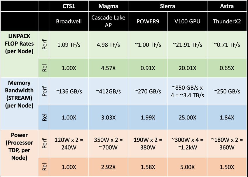
The range of power usage across all runs are summarized in Figure 2. The power usage on each platform for this
problem remains in a narrow band, relative to the spread of idle power and LinPACK. It is also apparent that the
processor TDP is not generally indicative of actual usage. The only clear commonality that can be seen in this data is
that the CTS-1 and Magma platforms have similar TDP to actual usage ratios, which have similar node designs.
On every platform with multiple runs, the runs with the fewest number of nodes is consistently the most energy efficient
and offer the highest throughput of work. Ares does not strong scale perfectly, so as the resources increase, the time
does not decrease proportionally. Although there is also a reduction in power per node as the code is strong scaled, it
does not reduce enough to offset the increased number of nodes used.
One common metric for comparing platforms is to use a node-to-node comparison. Due to limitations in the energy
measuring methodology (as discussed in Section 2), there aren’t exact node count matches across platforms. For
comparing Sierra to Astra, the closest available is Sierra’s 80 node run with Astra’s 72 node run. Comparing those two
data points shows that Sierra has a 3.3x speedup over Astra and that it is 1.4x more energy efficient. The ratio of node
power at these points is 2.15, which suggests that the speedup needed to reach breakeven on a GPU for this problem
is only 2.15. It should also be noted that at this point, the Sierra runs are strong scaled and less energy efficient than
its other runs.
For the same metric on the CPU platforms, Astra’s 72 node run and CTS-1’s 62 node run are the closest. For those
runs, there is a 1.3x speedup on Astra and Astra is 1.13x more energy efficient. The ratio of the power between the
two runs is 1.04, so the gain in efficiency is almost entirely from the faster runtime on Astra.
Another way to compare platforms is to look at equivalent node counts to get the same answer in the same amount of
time. Using this lens, the runs with the closest duration are Sierra’s 5 node run with Astra’s 72 node run and Sierra’s
10 node run with Astra’s 144 node run. In these cases, Sierra is about 5.5x more energy efficient than Astra for running
the same problem in the same amount of time. The ratio of node power between these runs is between 2.6 and 2.7,
which is more than offset by the 14x difference in nodes being used.
Table 2: Energy and time measurements gathered from the various platforms with Ares, running the same problem,
strong scaled across nodes.
Nodes Duration (s) Total Energy (kWh) Avg. Watts Per Node
CTS-1 62 28,424 167.56 342.28
Magma 48 17,094 212.41 931.96
Astra 72 20,851 148.37 356.71
144 12,705 181.28 355.7
Sierra 5 19,755 26.53 967.23
10 13,106 32.71 898.52
20 8,967 42.5 853.23
40 6,979 63.3 816.3
80 6,240 106.5 768.05
6Understanding Power and Energy Utilization in Large Scale Production Physics Simulation Codes
1750 Power ratio: [2.25-2.83]
1500 Power ratio: 2.72
Power per node (watts)
1250 Power ratio: [0.75-1.30]
1000
750
500 Power ratio: 1.04
250
0
CTS-1 Magma Astra Sierra Sierra
(GPU only)
Cluster
Figure 2: Ares power requirements (dark bars) relative to machine idle (lower whisker) and LinPACK power (upper
whisker) rates. Power ratio refers to the necessary speed up to break even in terms of energy usage compared to the
CTS-1 machine. Light colored bars correspond to processor TDP on each platform.
4.2 MARBL
MARBL’s cross platform study compares energy and power usage across the smallest number of nodes necessary
for the highest fidelity energy and power estimates. For the CPU based platforms, CTS-1, Magma, and Sierra, the
node counts were 62, 48, and 72 respectively. Prior to understanding the correction factor for Sierra, 360 nodes were
required to achieve the highest fidelity measurements.
Our starting point for the cross-platform analysis begins with understanding watts used for the simulation and the total
runtime. Table 3 reports the rate at which energy is consumed, while Figure 3 compares application power rates with
other known values.
1750 Power ratio: 3.05
1500 Power ratio: 2.68
Power per node (watts)
1250
1000
750
500 Power ratio: 1.12
250
0
CTS-1 Magma Astra Sierra
Cluster
Figure 3: MARBL power (dark bar) requirements relative to machine idle (lower whisker) and LinPACK power (upper
whisker) rates. Power ratio refers to the necessary speed up to break even in terms of energy usage compared to the
CTS-1 machine. Light colored bars corresponds to processor TDP for a given platform.
Table 3: Watts used in MARBL for 3D Triple point problem
Platform Nodes Duration (s) Avg. Watts Per Node Ratio of Watts used
relative to CTS-1
CTS-1 62 2,217 314 1x
Magma 48 1,024 842 2.68x
Astra 72 1,266 351 1.12x
Sierra 360 1,581 958 3.05x
7Understanding Power and Energy Utilization in Large Scale Production Physics Simulation Codes
To compare across platforms, we introduce the concept of a “CTS-1 work unit”. We define the CTS-1 work unit as
total number of quadrature points × cycles. Table 4 presents our observed energy usage along with throughput with
comparisons to the CTS-1 platform. After normalization, our findings show that relative to CTS-1 performance, the
GPU platform Sierra delivers a clear advantage in terms of improved energy efficiency (6.35x more efficient) and
throughput (19.37x). We also find that although Magma does utilize an energy quantity like the CTS-1 platform, it can
deliver an almost three-fold throughput performance (2.78x). Lastly, we find that Astra can provide reduced energy
usage (1.34x improvement to CTS-1) for a 1.5x throughput improvement.
Table 4: Cross platform study for MARBL using the 3D Triple point problem
Total Energy Throughput
Quadrature Throughput efficiency improvement
Platform Nodes Cycles Energy
points per kWh relative to relative to
(kWh)
CTS-1 CTS-1
CTS-1 62 4.68 · 108 500 12.02 1.92 · 1010 1x 1x
Magma 48 4.62 · 108 500 11.49 2.01 · 1010 1.04x 2.78x
Astra 72 4.62 · 108 500 8.91 2.59 · 1010 1.34x 1.5x
Sierra 360 3.7 · 109 5,000 151.5 1.22 · 1011 6.35x 19.37x
4.3 Imp
The Imp simulations were designed such that each run would take 60 to 80 minutes on each of three platforms: CTS-1,
Magma, and Sierra. Like the MARBL cross platform study, runs were designed to compare energy and power usage
across the smallest number of nodes necessary to gather the data.
Refer to Table 5 for a cross platform comparison of the watts/node used by Imp. Figure 4 compares the application
power rates with other known values.
To perform the comparison, we defined a work unit as the processing of 1e8 computational particles. We measured the
amount of work units completed, the seconds to solution, and the energy consumed. After normalization, we see that
relative to CTS-1 performance, the Sierra GPU is 2.33x more efficient. Also, Sierra provided 6.94x the throughput for
the 2D hohlraum simulation (see Table 6 for details).
Table 5: Watts used by Imp for 2D hohlraum simulation
Platform Nodes Work units Duration (s) Avg. Watts Per Node Ratio of Watts used
relative to CTS-1
CTS-1 62 9.9 3,947 340 1x
Magma 48 25.3 4,590 901 2.65x
Sierra 48 51.2 3,798 1,012 2.98x
Table 6: Cross platform study of 2D hohlraum simulation
Total Throughput Energy Throughput
Work Duration efficiency improvement
Platform Nodes Energy (kWh per
units (s) relative to relative to
(kWh) work unit)
CTS-1 CTS-1
CTS-1 62 9.9 3,947 23.12 2.33 1x 1x
Magma 48 25.3 4,590 55.14 2.18 1.06x 2.81x
Sierra 48 51.2 3,798 51.25 1 2.33x 6.94x
5 Optimization impact on power and energy on Sierra
5.1 Ares
To study the effects of optimization on power and energy on Sierra, we tested two optimizations. The first was to run
the code asynchronously as long as possible, where the unoptimized version would synchronize after every kernel.
8Understanding Power and Energy Utilization in Large Scale Production Physics Simulation Codes
1750 Power ratio: 2.98
1500 Power ratio: 2.65
Power per node (watts)
1250
1000
750
500
250
0
CTS-1 Magma Sierra
Cluster
Figure 4: Imp power requirements (dark bar) relative to machine idle (lower whisker) and LinPACK (upper whisker)
power rates. Power ratio refers to the necessary speed up to break even in terms of energy usage compared to the
CTS-1 machine. Light colored bars corresponds to processor TDP for a given platform.
The second was to perform kernel fusion on packing and unpacking kernels that are used to pack MPI communication
buffers. These are very small kernels that are kernel launch bound due to the small amount of data being moved per
kernel. This optimization is focused on improving strong scaling behavior. The results of the tests running with and
without all optimizations are presented in Figure 5 (and the data is presented in Table 7). As an additional baseline,
the code was also run utilizing only the CPU cores on the platform. For these CPU only runs, we subtracted out the
idle GPU power from Table 1 to have a fairer comparison.
As noted in the cross-platform section, we see that the energy consumption increases as we strong scale the problem
under all problem configurations. We also see that as we optimize the code, the strong scaling inefficiencies lessen,
which yields significantly lower energy usage at the highest node counts.
When we look at the data across the optimizations, we see that the optimizations all decrease the runtime of the problem
and generally reduce the overall energy consumption of the total run, except for the kernel fusion optimization at 1
or 2 nodes, where they had little effect. There is a trend in the data that as more optimizations are added, the power
increases. This is due to the optimizations eliminating gaps in between kernels, due to kernel launch overheads, which
keeps the GPU from idling, and thus does more work in a shorter amount of time. Although the power is increasing,
the runtime of the problems are decreasing faster, which leads to an overall gain in energy efficiency.
This data can also be used to discuss the energy breakeven point between using the CPU and the GPU. Most sim-
plistically, the ratio of the power used between two runs can be used to determine how much faster the code needs to
run to have the same energy consumption. In comparing all the GPU runs to the CPU runs, that ratio ranges between
1.15 and 1.42, depending on which node count is used. Comparing the 16 node unoptimized run to the CPU only
run confirms this, as their energy usage is almost equal with only being 1.13x faster. For every other comparison, the
GPUs are clearly far more energy efficient than using CPUs alone.
Another feature of the data to note is that although the vast majority of the compute and memory bandwidth are being
used by the GPU, the GPUs only account for 35-45% of the overall energy consumption of the node. This reinforces
that it is important to consider an entire architecture’s node design when looking at energy efficiency, rather than just
the compute units alone.
5.2 MARBL
To better understand the impact on power and energy on Sierra, we tracked power and energy usage on Sierra during
MARBL’s GPU porting effort. From inception, MARBL strictly used MPI for parallelism; thus, to run on GPU
platforms would require refactoring. We began tracking energy usage on Sierra shortly after reaching the performance
breakeven point between CPU and GPU runs, i.e. where we had comparable runtimes when running the same problem
on a CTS-1 node and on a Sierra node and utilizing the GPUs. We present our energy usage from May through October
2020 when exercising the shaped charge problem on a Sierra node. In general, we find that performance optimizations
can affect power usage differently. Figure 6(a) illustrates that although not all optimizations led to increased power,
there was a general downwards trend in total runtime. Total energy usage can be shown to decrease as the runtime
performance of the code improves as shown in Figures 6(b).
9Understanding Power and Energy Utilization in Large Scale Production Physics Simulation Codes
CPU only
214 No opt.
Fusion only
Runtime (s) [log2]
Async. only
213 Full opt.
212
211
20 21 22 23 24
Nodes [log2]
(a) Ares runtime
23 Total (CPU only)
Energy usage (kWh) [log2]
Total (No opt.)
Total (Fusion only)
22 Total (Async. only)
Total (Full opt.)
GPU (No opt.)
21 GPU (Fusion only)
GPU (Async. only)
GPU (Full opt.)
20
20 21 22 23 24
Nodes [log2]
(b) Ares energy usage
CPU only
800 No opt.
Average Watts per node
Fusion only
Async. only
700 Full opt.
600
500
20 21 22 23 24
Nodes [log2]
(c) Ares average power per node
Figure 5: Comparing the affects of several optimizations on Ares runtime (a), energy (b) and average power (c) in a
strong scaling study.
10Understanding Power and Energy Utilization in Large Scale Production Physics Simulation Codes
1,000 1,200
Avg. Watts per node 0.2 Total energy
Simulation run time 1,000 GPU energy
800
Energy usage (kWh)
800 0.15
Runtime (s)
600
Watts
600
0.1
400
400
200 0.05
200
0 0 0
9
9
6
7
8
0
6
7
8
0
-0
-0
-0
-0
-0
-1
-0
-0
-0
-1
20
20
20
20
20
20
20
20
20
20
20
20
20
20
20
20
20
20
20
20
Date Date
(a) MARBL power and runtime (b) MARBL energy usage
Figure 6: Tracked runtime, power and energy usage for MARBL’s 3D Shaped Charge problem during an active phase
of its GPU refactoring. Data was captured on a single node of Sierra (4 GPUs) between May and October 2020. (a)
Simulation average power usage (dashed blue line, using left axis) and runtime (red solid line, using the right axis).
(b) Energy usage across the entire node (dark blue) and restricted to the GPUs (magenta).
6 Conclusion
In this work we have presented a methodology based on actual computing system energy measurements for under-
standing power and energy consumption of production level scientific simulation codes. Using our methodology, we
performed studies using LLNL’s Ares, MARBL, and Imp codes. We found that it is imperative to perform energy
measurements, as using a surrogate such as processor TDP may overestimate power usage when running scientific
applications.
Additionally, we introduce the notion of the required speedup for an energy breakeven point between platforms.
Based on our experiments, we have found that Ares, MARBL, and Imp require 2-3x speedups on Sierra over a CTS-1
platform (node-to-node comparison) to reach the breakeven point between platforms. In practice, however these codes
achieve much greater speedups on a GPU based system compared to the CTS-1 platform thereby requiring less energy
to run on the GPU platform. For these problems Sierra was able to provide an energy savings of 2.33x for the Imp
code, 6.35x for MARBL, and 1.6-5x for Ares over the CTS-1 platform.
1750
1500
Power per node (watts)
1250
1000
750
500
250
0
CTS-1 Magma Astra Sierra Sierra
(GPU only)
Cluster
Figure 7: Application power requirements (dark bars) relative to machine idle (lower whisker) and LinPACK (upper
whisker) power rates. Light colored bars corresponds to processor TDP for a given platform.
Our studies also suggest that faster execution time tends to result in improved energy efficiency, but often with greater
power usage. Figure 7 illustrates the different power ranges for the applications comparing in addition to the idle and
LinPACK power rates. Finally, higher throughput correlates with higher energy efficiency.
11Understanding Power and Energy Utilization in Large Scale Production Physics Simulation Codes
Sierra Energy with Optimizations (kWh)
Unopt Async opt Fusion opt Full opt CPU only
1 node 1.80 1.77 1.92 1.80 X
2 nodes 2.14 2.00 2.15 1.98 6.92
4 nodes 2.86 2.41 2.72 2.45 7.26
8 nodes 4.14 3.35 3.63 3.23 7.17
16 nodes 7.70 5.50 6.22 4.76 7.50
Sierra GPU Energy with Optimizations (kWh)
Unopt Async opt Fusion opt Full opt CPU only
1 node 0.84 0.81 0.86 0.81 X
2 nodes 0.92 0.87 0.91 0.85 X
4 nodes 1.18 1.02 1.10 1.03 X
8 nodes 1.45 1.30 1.32 1.28 X
16 nodes 2.57 1.90 2.11 1.70 X
Sierra Average Watts per Node
Unopt Async opt Fusion opt Full opt CPU only
1 node 756 779 817 793 X
2 nodes 777 795 801 795 591
4 nodes 768 758 773 782 595
8 nodes 685 736 683 750 587
16 nodes 660 684 666 675 572
Sierra Duration (seconds)
Unopt Async opt Fusion opt Full opt CPU only
1 node 8572 8179 8463 8162 X
2 nodes 4977 4523 4839 4491 21084
4 nodes 3349 2859 3172 2819 10977
8 nodes 2720 2051 2388 1941 5491
16 nodes 2625 1807 2104 1587 2968
Table 7: Ares optimizations
Acknowledgments
We would like to thank Teresa Bailey, Jim Silva, Rob Neely and Brian Pudliner for their support in this work.
This work performed under the auspices of the U.S. Department of Energy by Lawrence Livermore National Labora-
tory under Contract DE-AC52-07NA27344. LLNL-TR-828702.
Sandia National Laboratories is a multimission laboratory managed and operated by National Technology and Engi-
neering Solutions of Sandia, LLC., a wholly owned subsidiary of Honeywell International, Inc., for the U.S. Depart-
ment of Energy’s National Nuclear Security Administration under contract DE-NA0003525.
A Ares optimization data
Table 7 lists the data from the charts in Figure 5.
References
[1] https://www.top500.org/lists/green500. URL https://www.top500.org/lists/green500/.
[2] Y. Abe, H. Sasaki, M. Peres, K. Inoue, K. Murakami, and S. Kato. Power and performance analysis of GPU-
accelerated systems. In 2012 Workshop on Power-Aware Computing and Systems (HotPower 12), 2012.
12Understanding Power and Energy Utilization in Large Scale Production Physics Simulation Codes
[3] D. C. Price, M. A. Clark, B. R. Barsdell, R. Babich, and L. J. Greenhill. Optimizing performance-per-watt on
GPUs in high performance computing. Computer Science-Research and Development, 31(4):185–193, 2016.
[4] J. Enos, C. Steffen, J. Fullop, M. Showerman, G. Shi, K. Esler, V. Kindratenko, J. E. Stone, and J. C. Phillips.
Quantifying the impact of GPUs on performance and energy efficiency in HPC clusters. In International Con-
ference on Green Computing, pages 317–324. IEEE, 2010.
[5] T. Patel, A. Wagenhäuser, C. Eibel, T. Hönig, T. Zeiser, and D. Tiwari. What does power consumption behavior
of HPC jobs reveal?: Demystifying, quantifying, and predicting power consumption characteristics. In 2020
IEEE International Parallel and Distributed Processing Symposium (IPDPS), pages 799–809. IEEE, 2020.
[6] S. Kamil, J. Shalf, and E. Strohmaier. Power efficiency in high performance computing. In 2008 IEEE Interna-
tional Symposium on Parallel and Distributed Processing, pages 1–8. IEEE, 2008.
[7] R. E. Grant, S. D. Hammond, J. H. Laros III, M. Levenhagen, S. L. Olivier, K. Pedretti, H. L. Ward, and A. J.
Younge. Enabling power measurement and control on Astra: The first petascale arm supercomputer.
[8] R. E. Grant, M. Levenhagen, S. L. Olivier, D. DeBonis, K. T. Pedretti, and J. H. Laros III. Standardizing power
monitoring and control at exascale. Computer, 49(10):38–46, 2016.
[9] D. A. Beckingsale, J. Burmark, R. Hornung, H. Jones, W. Killian, A. J. Kunen, O. Pearce, P. Robinson, B. S.
Ryujin, and T. R. W. Scogland. RAJA: Portable performance for large-scale scientific applications. In 2019
IEEE/ACM international workshop on performance, portability and productivity in HPC (p3hpc), pages 71–81.
IEEE, 2019.
[10] D. A. Beckingsale, M. J. Mcfadden, J. Dahm, R. Pankajakshan, and R. D. Hornung. Umpire: Application-focused
management and coordination of complex hierarchical memory. IBM Journal of Research and Development, 64
(3/4):00–1, 2019.
[11] A. Vargas, T. Stitt, K. Weiss, V. Tomov, J.-S. Camier, Tz. Kolev, and R. Rieben. Matrix-free approaches for
gpu acceleration of a high-order finite element hydrodynamics application using mfem, umpire, and raja. arXiv
preprint arXiv:2112.07075, 2021.
[12] J. D. Bender, O. Schilling, K. S. Raman, R. A. Managan, B. J. Olson, S. R. Copeland, C. L. Ellison, D. J.
Erskine, C. M. Huntington, B. E. Morgan, and et al. Simulation and flow physics of a shocked and reshocked
high-energy-density mixing layer. Journal of Fluid Mechanics, 915:A84, 2021. doi: 10.1017/jfm.2020.1122.
[13] R. Anderson, A. Black, B. Blakeley, R. Bleile, J.-S. Camier, J. Ciurej, A. Cook, V. Dobrev, N. Elliott, J. Grondal-
ski, C. Harrison, R. Hornung, Tz. Kolev, M. Legendre, W. Liu, W. Nissen, B. Olson, M. Osawe, G. Papadimitriou,
O. Pearce, R. Pember, A. Skinner, D. Stevens, T. Stitt, L. Taylor, V. Tomov, R. Rieben, A. Vargas, K. Weiss,
D. White, and L. Busby. The Multiphysics on Advanced Platforms Project. Technical report, LLNL-TR-815869,
LLNL, 2020.
[14] R. D. Hornung, A. Black, A. Capps, B. Corbett, N. Elliott, C. Harrison, R. Settgast, L. Taylor, K. Weiss, C. White,
and G. Zagaris. Axom, Oct. 2017. URL https://github.com/LLNL/axom.
[15] R. Anderson, J. Andrej, A. Barker, J. Bramwell, J.-S. Camier, J. Cerveny, V. Dobrev, Y. Dudouit, A. Fisher,
Tz. Kolev, W. Pazner, M. Stowell, V. Tomov, I. Akkerman, J. Dahm, D. Medina, and S. Zampini. MFEM: A
modular finite element methods library. Computers & Mathematics with Applications, 81:42–74, 2021. doi:
10.1016/j.camwa.2020.06.009.
[16] P. S. Brantley, N. A. Gentile, M. A. Lambert, M. S. McKinley, M. J. O’Brien, and Walsh J. A. A new implicit
Monte Carlo thermal photon transport capability developed using shared Monte Carlo infrastructure. The Inter-
national Conference on Mathematics and Computational Methods Applied to Nuclear Science and Engineering,
Portland, Oregon, August 25-29, 2019, 2019.
[17] J.A. Fleck Jr and J.D. Cummings Jr. An implicit Monte Carlo scheme for calculating time and frequency depen-
dent nonlinear radiation transport. Journal of Computational Physics, 8(3):313–342, 1971.
[18] B. C. Yee, S. S. Olivier, B. S. Southworth, M. Holec, and T. S. Haut. A new scheme for solving high-order
DG discretizations of thermal radiative transfer using the variable Eddington factor method. arXiv preprint
arXiv:2104.07826, 2021.
13You can also read