Upgraded antennas for pulsar observations in the Argentine Institute of Radio astronomy
←
→
Page content transcription
If your browser does not render page correctly, please read the page content below
A&A 633, A84 (2020)
https://doi.org/10.1051/0004-6361/201936525 Astronomy
c ESO 2020 &
Astrophysics
Upgraded antennas for pulsar observations in the Argentine
Institute of Radio astronomy
G. Gancio1 , C. O. Lousto2 , L. Combi1,2 , S. del Palacio1 , F. G. López Armengol1,2 , J. A. Combi1,3 , F. García4,1 ,
P. Kornecki1 , A. L. Müller1 , E. Gutiérrez1 , F. Hauscarriaga1 , and G. C. Mancuso1
1
Instituto Argentino de Radioastronomía (IAR), C.C. No. 5, 1894 Buenos Aires, Argentina
e-mail: ggancio@iar.unlp.edu.ar
2
Center for Computational Relativity and Gravitation, School of Mathematical Sciences, Rochester Institute of Technology,
85 Lomb Memorial Drive, Rochester, NY 14623, USA
e-mail: colsma@rit.edu
3
Facultad de Ciencias Astronómicas y Geofísicas, Universidad Nacional de La Plata, Paseo del Bosque, B1900FWA La Plata,
Argentina
4
Kapteyn Astronomical Institute, University of Groningen, PO Box 800, 9700 Groningen, The Netherlands
Received 19 August 2019 / Accepted 29 November 2019
ABSTRACT
Context. The Argentine Institute of Radio astronomy (IAR) is equipped with two single-dish 30 m radio antennas capable of perform-
ing daily observations of pulsars and radio transients in the southern hemisphere at 1.4 GHz.
Aims. We aim to introduce to the international community the upgrades performed and to show that the IAR observatory has become
suitable for investigations in numerous areas of pulsar radio astronomy, such as pulsar timing arrays, targeted searches of continuous
gravitational waves sources, monitoring of magnetars and glitching pulsars, and studies of a short time scale interstellar scintillation.
Methods. We refurbished the two antennas at IAR to achieve high-quality timing observations. We gathered more than 1000 h of
observations with both antennas in order to study the timing precision and sensitivity they can achieve.
Results. We introduce the new developments for both radio telescopes at IAR. We present daily observations of the millisecond pulsar
J0437−4715 with timing precision better than 1 µs. We also present a follow-up of the reactivation of the magnetar XTE J1810–197
and the measurement and monitoring of the latest (Feb. 1, 2019) glitch of the Vela pulsar (J0835–4510).
Conclusions. We show that IAR is capable of performing pulsar monitoring in the 1.4 GHz radio band for long periods of time with
a daily cadence. This opens up the possibility of pursuing several goals in pulsar science, including coordinated multi-wavelength
observations with other observatories. In particular, daily observations of the millisecond pulsar J0437−4715 would increase the sen-
sitivity of pulsar timing arrays. We also show IAR’s great potential for studying targets of opportunity and transient phenomena, such
as magnetars, glitches, and fast-radio-burst sources.
Key words. instrumentation: detectors – methods: observational – pulsars: general – telescopes
1. Introduction Monitoring in Argentina3 (PuMA) team is a collaboration of sci-
entists and technicians from the IAR and the Rochester Institute
The Argentine Institute of Radio astronomy (IAR; Instituto of Technology (RIT). The collaboration has been working for
Argentino de Radioastronomía1 ) was founded in 1962 as a two years with both antennas, including the implementation of a
pioneer radio observatory in South America with two 30 m dedicated backend, the construction of a brand new frontend for
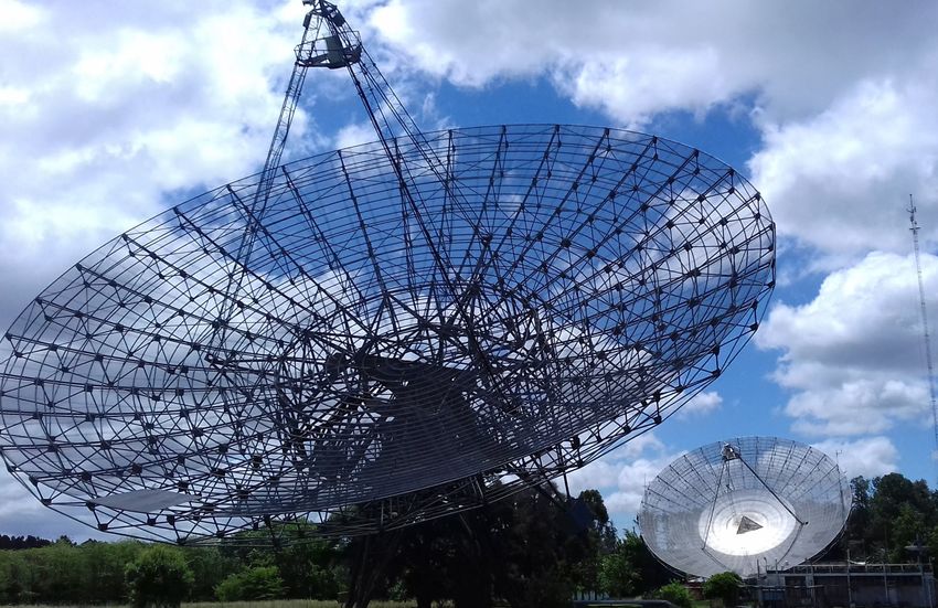
parabolic single-dish radio antennas (Fig. 1). Antenna 1 (A1) A2, in addition to the formation of human resources for obser-
saw its first light in 1966, whereas Antenna 2 (A2) was built vations, data analysis, and pulsar astrophysics. This project rep-
later in 19772 . The IAR’s initial purpose was to perform a resents the first systematic pulsar timing observations in South
high sensitivity survey of neutral hydrogen (λ = 21 cm) in the America and the beginning of pulsar science in Argentina.
southern hemisphere; this survey ended satisfactorily in the year In this work, we present the new hardware developments and
2000 with high-impact publications in collaboration with Ger- observations of IAR’s radio antennas from the last two years.
man and Dutch institutions (Testori et al. 2001; Bajaja et al. In Sect. 2, we give an overview of the current state of the radio
2005; Kalberla et al. 2005). observatory, its radio interference environment (RFI), the atomic
Although the IAR has been a center of intense scientific and clock availability, and the new developments for the acquisition
technological activity since it was founded, the radio antennas software. In Sect. 3, we describe the observational techniques
have not been employed in any scientific project since 2001. For and capabilities, both hardware and observational cadence, as
the first time in over fifteen years, the IAR antennas are being well as their automation. The calibration of total flux densities
upgraded to conduct high-quality radio astronomy. The Pulsar and polarization are part of our current developments.
In Sect. 4, we give a description of the various scien-
1
http://www.iar.unlp.edu.ar tific projects that are being carried out or will be in the near
2
In 2019, A1 and A2 were baptized “Varsavsky” and “Bajaja”, respec-
3
tively, in honor to their contributions to the IAR. http://puma.iar.unlp.edu.ar
Article published by EDP Sciences A84, page 1 of 12A&A 633, A84 (2020)
than A2 in the range 1150–1450 MHz, model ZX75BP-1280+
from Mini-circuits4 .
The backend or acquisition module is based on two SDRs
model B205 from Ettus5 using a Xilinx Spartan-6 XC6SLX75
field-programmable gate array (FPGA). This allows us to
acquire raw samples from the front-end intermediate frequency
as voltages in time series with a maximum rate of 56 MHz per
board, and a universal serial bus (USB) 3.0 for connectivity.
The sample rate is the same as the analog bandwidth due to the
internal frontend in the SDR module. As each receiver has two
digitizer boards, each with 56 MHz of bandwidth; we can use
them in two modes: (i) as consecutive bands, giving a total of
112 MHz of bandwidth for a single polarization; (ii) by adding
the two polarizations of 56 MHz bandwidth in order to obtain
Fig. 1. View of IAR antennas, A2 (left) and A1 (right). total power. A1 currently uses the first configuration.
The surface of A1 consists of a solid area at the center of the
parabolic surface, while the rest is made of perforated aluminum
future with further hardware improvements. One of the major sheets. This configuration gives an aperture efficiency of 32.8%
goals of the PuMA collaboration involves high-cadence mon- (Testori et al. 2001).
itoring of millisecond pulsars (MSPs). In particular, monitor-
ing of PSR J0437−4715 (one of the closest MSPs) is of great 2.2. Antenna 2
importance for gravitational wave detection using pulsar timing
array techniques. Other close-by MSPs are also a target of the A2 has a newly developed receiver that is fully operational since
LIGO-Virgo collaboration for the search of continuous gravita- November 2018. The receiver, different from the one in A1, has
tional waves. In addition, interstellar scintillation can be studied the digitization stage directly in the RF band, having as a result
with the same kind of data used at different time scales. Also, less RF components and more RF bandwidth available at lower
transient phenomena, such as fast radio bursts (FRBs), magne- cost. The RF feeder uses a turnstile feed with two orthogonal cir-
tars, and pulsar glitches are recent additions to the goals of our cular polarization outputs, each output is connected to the SDRs
observations. Lastly, we discuss in Sect. 5 the impact that our through their low noise amplifiers and filters.
contributions to radio observations in the southern hemisphere The backend of A2 has the same scheme as A1 but with a
may have on those areas of current astrophysical research, and different configuration. For A2, both SDR boards take data of
the potential for near-term improvement in both hardware and each circular polarization at the same time, frequency and band-
software. width. The processing software adds both polarizations to obtain
total power. At the present time, we are not processing the polar-
ization products as Stokes parameters, though this will be imple-
2. The IAR observatory mented in the processing software shortly.
A2 has a wider range of sensitivity, including higher frequen-
Located in the provincial park Pereyra Iraola near the city of La cies up to 1600 MHz, with the use of a filter model VBFZ-1400-
Plata, Buenos Aires, the IAR itself is located at −34◦ 510 5700. 35 S+, also from Mini-circuits6 (Fig. 3). The surface of A2 presents
(latitude) and 58◦ 080 2500. 04 (longitude), with local time UTC-3. a grid mesh for all its surface, giving a worse figure for its aper-
The IAR observatory has two 30 m diameter single-dish anten- ture efficiency, therefore resulting in a different Gain; the esti-
nas, A1 and A2, aligned on a north-south direction (Fig. 1), sepa- mated aperture efficiency for A2 is 30.0%. The characteristics of
rated by 120 m. These radio telescopes cover a declination range the current frontend in A2 are listed in Table 1.
of −90◦ < δ < −10◦ and an hour angle range of two hours east-
west, −2h < t < 2h. The angular resolution at 1420 MHz is
∼300 . The block diagram of Fig. 2 represents the connections of 2.3. Clock synchronization
the antennas with their different modules. Clock synchronization of the digital boards is performed with the
one pulse per second (PPS) signal of a global positioning system
2.1. Antenna 1 (GPS) disciplined oscillator with an accuracy of 1.16 × 10⁻¹²
(one-day average). In order to get a precise data time stamp,
Since 2004, several updates and repairs were made on A1, the PPS signal is used in the SDR boards to synchronize the
including a complete front-end repair in 2009 and a new set of first time sample with the exact second of the GPS time. Then,
positional encoders installed in 2014 to keep the tracking system the acquisition software reads the computer clock, which is syn-
up to date. In 2015, we installed a software defined radio (SDR) chronized with a Network Time Protocol (NTP) and a PPS sig-
module to perform pulsar observations. The characteristics of the nal from the GPS directly connected to the kernel OS through a
current frontend of A1 are listed in Table 1. serial port.
The frontend has as a feeder system a orthomode transducer
(OMT) with a quadridge type wave guide to coax transducer,
using a 90◦ hybrid coupler it gives both circular polarization 4
https://www.minicircuits.com/WebStore/dashboard.
products (LHC and RHC) from the linear products. Currently html?model=ZX75BP-1280-S%2B
only one circular polarization is used. We have inserted new 5
https://www.ettus.com/all-products/
band pass radio frequency (RF) filters into the receivers of both usrp-b200mini-i-2/
antennas; the rest of the analog chain corresponds to a standard 6
https://www.minicircuits.com/WebStore/dashboard.
heterodyne receiver. A1 benefits from a lower insertion loss filter html?model=VBFZ-1400-S%2B
A84, page 2 of 12G. Gancio et al.: Upgraded antennas for pulsar observations in the Argentine Institute of Radio astronomy
Receivers at each Antenna Front-End
N.D.
LNA LNA MIXER IF-AMP Ctrl&Tlmy
CPU
Digital I.F.
Back-End 3
Back-End
FO
LO-Input
L.O.
Sync-PPS
F.O. LAN
Encoders-
Redout Encoders-
Redout
Motor
RT-II Ctrl RT-I
Motor
Ctrl
Time & Frequency
Control AI & AII
Distribution Digital Back-End 1 Local Oscillator Digital Back-End 2
“Pointing”
GPS Based
LAN LAN LAN LAN
Sync_Sidereal_Time
GPS_10MHz
PPS_GPS
10MHz CW Hydrogen Maser
1Km Analogue Fiber Optic Link Control Room
Fig. 2. Current setup of IAR antennas.
At less than one kilometer away from the IAR the Argentine- density (PSD) [dBW m−2 Hz−1 ] (Fig. 4). Moreover, the IAR has
German Geodetic Observatory is located, AGGO7 , dedicated, implemented a new protocol to provide a clean RFI local envi-
among other research, to Very Large Baseline Interferometry ronment that is compatible with the current research and techni-
observations of quasars for geodetic purposes. This kind of mea- cal activity of the nearby antennas.
surements requires a precise clock for the synchronization with Observations with A1 have shown that RFIs affect ∼10%
other observatories. This is achieved using an hydrogen maser of the daily observing time, although during night-time the RFI
clock with a short time stability of 10−15 (Allan Variance). With activity reduces significantly and compromises less than 1% of
a locally developed RF-Over-Fiber device (Mena et al. 2013), we the observing time. In average, observations with A2 have a sig-
receive the 10 MHz signal from the AGGO’s hydrogen maser nificant less amount of RFI due to its distance to the administra-
using a fiber optic cable that connects both institutions. This tive offices and laboratories.
signal is used to synchronize a test unit backend with the aim Narrow-band mitigation is performed with the rfifind
to compare results from the different time bases used at the package from PRESTO9 . First, the software parses the data in
moment. In the future, this shall be used to synchronize the data pieces of a certain time width (1 s in our case) per frequency
acquisition. interval. Then, it identifies in each one of these pieces weather
the total power is too high, the data have an abnormal standard
deviation, or the average of the data is above some given thresh-
2.4. Radio-Frequency-Intereference environment
old. In that case, a mask is applied to the data before it is pro-
The IAR is located in a rural area outside La Plata, Buenos Aires. cessed. In Fig. 5 we present an example mask for A1 and A2
Although this is not a radio frequency interferences (RFI) quiet that shows the flagged data as a function of time and frequency
zone, the radio band from 1 GHz to 2 GHz has a low level of channel. We note that A1 is more affected by random RFIs due
RFI activity that ensures the capability to do radio astronomy8 , to its local environment. These RFIs are usually mitigated dur-
as confirmed by the latest RFI measurement campaign from ing night time, out of office hours. In the case of A2, the RFIs are
December 2017 (Gancio et al. 2014) for over a month in which predominantly monochromatic and their impact can be mitigated
the 90 % of RFIs are detected below the −160 power spectral by using a larger number of frequency channels. We also note
that these RFIs were proven to be polarized, so it is not straight-
7
http://www.aggo-conicet.gob.ar forward to compare the masks from A1 and A2. Moreover,
8
Argentina is a member of the International Telecommunication
9
Union that protects radio bands for astronomical observations. https://www.cv.nrao.edu/~sransom/presto/
A84, page 3 of 12A&A 633, A84 (2020)
Table 1. Parameters of the antennas and their receivers (frontend and −130
10 %
software configuration). 90 %
−140 Max
Med
Min
Parameter A1 A2 −150
PSD [dBW/m2/Hz]
Antenna diameter 30 m
FWHM at 1420 MHz 300 −160
Mounting Equatorial
Maximum tracking time 220 min −170
Low noise amplifiers (a) HEMT He E-PHEMT −180
Filters range (MHz) 1100−1510 1200−1600
Electronics bandwidth 110 MHz 200 MHz −190
Polarization One circular Two circular
Receiver temperature 100 K 110 K 1 1.1 1.2 1.3 1.4 1.5
Aperture efficiency (b) 32.8% 30% ν [GHz]
Gain (b) (Jy K−1 ) 11.9 13.02 Fig. 4. Wide bandwidth Power Spectrum Density obtained from a one-
Calibration Noise injection at feed month average of measurements to characterize the RFI environment at
Instantaneous bandwidth 112 MHz 56 MHz IAR.
Polarization product One (circular) Total power
SDR models B210 – B205-mini-i
Boards per CPU Two
Max data rate per 54 KHz
Reference input PPS
Computer CPU i7, NVMe 1.2
PCIe Gen 3 × 2 SDD
Software language C
Notes. (a) At room temperature. (b) Values from Testori et al. (2001).
15
VBFZ−1400−S+
ZX75BP−1280−S+
Insertion Loss (dB)
10
5
0
1000 1200 1400 1600 1800
Frecuency (MHz)
Fig. 3. RF filters installed in A1 (ZX75BP-1280-S+) and A2 (VBFZ-
1400-S+).
the mask criteria applies differently in each antenna given their Fig. 5. Example of a 3.5 h RFI mask for A1 (top) and A2 (bottom) for
different sensibility. A more detailed analysis of this RFI envi- a simultaneous observation using rfifind with -time 1 and default
ronment is ongoing. parameters; colored sections are masked out. The mask criteria acts dif-
ferently in each antenna given their different sensibility, so the plots
are not in the same scale. RFIs affect only 1.3% of this observation for
2.5. Future upgrades A1 and less than 6.3% for A2. We note that the persistent RFIs in A2
We plan to increase the bandwidth of the receivers. This implies: are monochromatic and affect individual channels only (2 of 64 in this
case). The frequency channels on the borders of the bandwidth in A2
(i) an upgrade of the frontend to be able to operate in a frequency
are removed due to the design of the receiver.
band from 1 GHz up to 2 GHz with insertion losses below 1 dB;
(ii) a new backend based on the CASPER boards like the SNAP
board10 with bandwidths up to 500 MHz for each polarization.
3. Observations
Moreover, the new receiver will benefit from state-of-the-art
low-noise-amplifiers and electronics that will allow to reduce 3.1. Software infrastructure
the system temperature to T sys < 50 K (using its cryogenic
capability). The acquisition software was developed entirely at the IAR in C
language. It processes the raw voltage samples at the desired rate
without losses, while transforming them into a time series of RF
10
https://github.com/casper-astro/casper-hardware/ channels. The software uses a scheme of synchronized threads
blob/master/FPGA_Hosts/SNAP/README.md in order to read the time samples from the different boards,
A84, page 4 of 12G. Gancio et al.: Upgraded antennas for pulsar observations in the Argentine Institute of Radio astronomy
Read Setup_file
.FIL header write
Manager Scheduler
SDR Setup
CLI
PPS time syncronization (Antenna Chat)
User Controlled
Events Log
Environment
WEB UI
Wait for PPS on all board to
start acquisition
Network
Receive Packet-0 of m time
samples from Board 0 & 1
Antenna Antenna Weather Raw Data
... Receiver Mount Station Storage
Radio Telescope Control Modules
Receive Packet n of m time samples from
Main Thread
Board 0 & 1
Fig. 7. Software architecture for the control of the radio telescopes.
Write to
Process Thread FFT of Channelize
disk
Packet n-1 Packet n-1
Packet n-1 We are working in upgrading the current client-server archi-
tecture by means of building a scalable and dynamic control
Last Process FFT of Channelize
Write to software that consists on a series of simple modules that per-
disk
Thread Packet n Packet n
Packet n
form specific tasks. These modules can be orchestrated by states,
events and messages passed to a controller software that has
enough privileges to make decisions upon the running modules.
This common communication interface/application program-
Close .FIL file
ming interface (API) allows the use of graphical user interfaces
(GUIs), command line interfaces (CLIs), and simple viewers. A
scheme of the software architecture is shown in Fig. 7.
Finally, we plan to develop a scheduler to fully automate
Close SDR
observations in order to offer the whole observation pipeline to
the scientific community. In addition, the IAR is preparing a pub-
Fig. 6. Pulsar software data acquisition block. lic proposer’s interface together with online tools to assess the
technical aspects of a requested observation and a remote moni-
toring during its performance.
process the fast Fourier transform (FFT) products, do the time
average, and separate the final data product into channels before
3.3. Data processing
writing to disk. This is performed while keeping the syn-
chronization with the PPS signal from the GPS Disciplined As we mentioned before, we apply PRESTO to process the Fil-
Oscillator (GPSDO). The final product is a file in Filterbank terbank files acquired. First, we employ the rfifind routine to
(SIGPROC) format11 , compatible with standard pulsar reduc- generate a mask, which allows us to remove the RFIs. Then,
tion software like PRESTO (Ransom 2001; Ransom et al. 2002, using that mask, we fold the data with prepfold. For this step,
2003). Figure 6 represents the software diagram used in the C we use the ATNF catalog12 (Manchester et al. 2005), data as
code, and Table 1 summarizes the main parameters of the digital input. The outputs of the last routine are a set of prepfold
receiver and the configuration used on each antenna. (.PFD) files.
Tracking and pointing systems of A1 and A2 are controlled For the moment we are working on three different projects:
remotely through the IAR server. A weather station and a video- detection of glitches, pulse time of arrival (ToA) extraction, and
camera help to control the IAR environment. Data acquisition flux density measurement. In the case of a glitch search, we ana-
is performed by a different computer, connected to the back- lyze if the pulsar observed period matches with the expected
ends. After acquisition, Filterbank files are saved and processed topocentric period for the observing date derived from the lat-
in the IAR storage system. The raw data files are also transferred est reported ephemeris in the ATNF catalog.
to a data center at the Rochester Institute for Technology (RIT- If it is not the case, we reprocess the Filterbank file doing a
PuMA-DEN Lab) for backup. fitting for the new period (see Sect. 4.4). The extraction of ToAs
is handled with the PSRCHIVE (Hotan et al. 2004) package pat.
These ToAs are processed with TEMPO2, using a suitable tem-
3.2. Automation
plate for the pulse profile, to compute residuals needed for our
We are developing a distributed software architecture to control scientific goals (see Sect. 4.1). The third project is the calibra-
both IAR radio telescopes. Our goal is to generate a modern, tion of pulsar flux densities. For that, we employ the diode tube
dynamic and heterogeneous system in which modularity is an in each of our radio telescopes and calibration sources, such as
essential part, both in the development and in the expansion of Hydra A. Figure 8 shows a summary of the whole reduction
the tools available for the observatory. process of the data.
11 12
http://sigproc.sourceforge.net http://www.atnf.csiro.au/research/pulsar/psrcat/
A84, page 5 of 12A&A 633, A84 (2020)
500
Back-end rfifind post-upgrade
RFI mask
raw-data 400 pre-upgrade
Acquisition
software PRESTO 300
S/N
filterbank Folding &
file dedispersion 200
prepfold
100
PFD files 0
60 80 100 120 140 160 180 200 220
Duration [minutes]
PSRCHIVE 1.0 T=171 min T=187 min
diode tube + S/N= 23 S/N= 221
calib source 0.8
Normalized Flux
0.6
ToAs
0.4
Pulsar Pulsar
period flux 0.2
TEMPO2 + model
0.0
Residuals 0.0 0.2 0.4 0.6 0.8 1.0 0.0 0.2 0.4 0.6 0.8 1.0
Fraction of pulsar period Fraction of pulsar period
Fig. 8. Data processing summary. Fig. 9. Top panel: signal-to-noise distribution as a function of the inte-
gration time for different observations of J0437−4715 before and after
Further post-processing is carried out with the freely avail- the upgrade in A1. Bottom panel: typical pulse profiles in the pre-
upgrade and post-upgrade configuration.
able PyPulse package13 . For instance, we make use of this pack-
age to compute the signal-to-noise ratio of our observations
defined as the ratio between the mean pulse peak and the rms of Our main target for testing purposes is the bright
the noise. The latter is calculated from an off-pulse window of MSP J0437−4715 (Fig. 9). This pulsar allows us to test the tim-
size 1/8 of the total phase bins in which the integrated flux den- ing quality of both antennas thanks to its high timing stability,
sity is minimal. We refer to Lam et al. (2016) for further details. high brightness, and short spin period. In Fig. 9, we compare
our observations of J0437−4715 in the pre-upgrade and post-
3.4. Observational capabilities and testing upgrade configuration. The upgrade consisted in an increase in
bandwidth from 20 to 112 MHz, the incorporation of a better
We have been observing with both antennas since December band-pass filter, and the use of both digitizer boards.
2018 to test and calibrate them. Both radio telescopes are capable We note that this pulsar shows an important variation of the
of observing sources for almost four hours on a daily basis. We flux due to scintillation (Osłowski et al. 2014), most notably in
note that bright pulsars with sharp-peaked profiles are the eas- observations after the upgrade which have a larger bandwidth.
iest to detect; this is straightforward from the standard formula We show the preliminary timing results in the next section.
for the expected signal-to-noise ratio (S/N; Lorimer & Kramer
2012):
p r 3.5. Collaborations with other radio observatories in
np tobs B P − W Argentina
S /N . Smean , (1)
GT sys W One spin-off from the development of the digital back-end
where Smean , P, and W are the mean flux density, period and receiver is its use as a stand alone unit for radio astronomical
equivalent width of the pulses, respectively, G, B, np , and T sys observations. This unit has been tested successfully in a 35 m
are the antenna gain, bandwidth, number of polarizations, and Deep Space Antenna (DSA) named CLTC-CONAE-Neuquen15 ,
system temperature, respectively, and tobs is the effective observ- installed in Neuquen, Argentina. Test observations were car-
ing time. Using Eq. (1) we can estimate which pulsars can be ried out in S and X bands targeting both pulsars (Vela and
observed with IAR antennas. We introduce the parameters given J0437−4715) and continuum sources. This will enable the pos-
in Table 1 in the equation and we set the maximum observ- sibility to do simultaneous observations between the IAR radio
ing time to t = 220 min, from where we obtain a value for telescopes and the DSA antenna at different frequencies for radio
the expected S/N. Considering that a reliable detection can be astronomical research.
achieved for those pulsars with a S /N > 10, we make use of the
python tool psrqpy (Pitkin 2018) to select the ones that IAR’s
antennas are capable to detect14 . 4. Enabling science projects
13
https://github.com/mtlam/PyPulse In this section we describe several scientific projects that we are
14
We note that this estimated way to calculate the signal-to-noise corre- –or will be– able to perform with the refurbished IAR antennas.
sponds to the S/N as computed with a cross-correlation function instead
15
of the peak to off-peak rms S/B, see Lam et al. (2016) to the mathemat- https://www.argentina.gob.ar/ciencia/conae/
ical relation between the two quantities. centros-y-estaciones/estacion-cltc-conae-neuquen
A84, page 6 of 12G. Gancio et al.: Upgraded antennas for pulsar observations in the Argentine Institute of Radio astronomy
We present the current state of each project, some preliminary 3
A1 (rms = 0.56 µs)
results, and projections with future hardware improvements. A2 (rms = 0.81 µs)
2
4.1. Pulsar timing and gravitational waves
1
Residual [µs]
Millisecond pulsars show a remarkable rotational stability. This
allows one to predict the TOA of their pulses with high pre- 0
cision over long periods of time. Given a physical model, we
can compare the predicted TOAs, tP , with the actual observed −1
TOAs in a certain reference frame, tO , and compute the residuals
δt = tP − tO . The residuals contain information of the astrophys- −2
ical system and small effects due to different processes that can
be incorporated in the timing model. For millisecond pulsars in
−3
particular, the residuals are dominated by white-noise when a −90 −60 −30 0 30 60 90
large-enough bandwidth is used to resolve accurately the disper- MJD−58680 [days]
sion measure and can reach the order δt < 1 µs.
Fig. 10. Residuals of the ToAs of the pulsar J0437−4715 measured at
With this idea, pulsar timing arrays (PTAs), consisting usu- IAR with A1 and A2. The residuals and rms have been computed with
ally of tens of precisely-timed MSPs, can be used as a Galac- the TEMPO2 package (Hobbs et al. 2006) and error bars correspond
tic scale detector of low-frequency gravitational waves. The only to template-fitting errors (i.e., no systematics considered).
main goal is to detect a “stochastic background” of such low-
frequency gravitational waves, originated from an ensemble Table 2. Observable MSPs from IAR with the current setup (top) and
of unresolved supermassive black hole binaries (SMBHBs). with future upgrades (bottom).
Specifically, the effect of this background would appear in the
PTA as a particular spatial angular correlation of the ToAs from
different pulsars given by the Hellings-Downs curve (Hellings J name P0 S1400 W50 (a) S /N (b) D DM
[ms] [mJy] [ms] [kpc] [pc cm−3 ]
& Downs 1983). Several physical effects need to be modeled
and corrected in order to find the effect of gravitational waves J0437−4715 5.757 150.2 0.141 336 (c) 0.16 2.64
on the ToAs; chiefly, the pulsar dynamics and intrinsic insta- J1744−1134 4.075 3.2 0.137 15.1 0.15 3.14
bilities, timing delays due to the interstellar medium and solar J2241−5236 2.187 1.95 0.07 9.4 0.96 11.41
wind (see Hobbs & Dai 2017, for a recent review). There are J1643−1224 4.622 4.68 0.314 15.26 0.79 62.41
J1600−3053 3.598 2.44 0.094 13.1 2.53 52.33
three main PTA collaborations, NANOGrav from North America
J2124−3358 4.931 4.5 0.524 11.5 0.36 4.60
(Arzoumanian et al. 2018), EPTA from Europe (Desvignes et al. J1603−7202 14.84 3.5 1.206 10.4 1.13 38.05
2016), and PPTA from Australia (Reardon et al. 2016), together J1730−2304 8.123 4.00 0.965 9.6 0.51 9.62
with an international PTA consortium (IPTA; Verbiest et al. J0900−3144 11.11 3.00 0.8 9.5 0.38 75.71
2016) that coordinates common efforts. Observatories in China, J0711−6830 5.491 3.7 1.092 6.5 0.11 18.41
South Africa, India, and Argentina plan to join the IPTA soon. J1933−6211 3.543 2.30 0.36 6.0 0.65 11.52
Bright MSPs, such as PSR J0437−4715, are excellent tar- J1652−48 3.785 2.70 * * 4.39 187.8
gets for IAR’s antennas. We are currently performing an almost
four hours per day monitoring of PSR J0437−4715 at 1400 MHz. Notes. P0 is the barycentric period of the pulsar, S1400 the mean flux den-
sity at 1400 MHz, W50 the pulse width at 50% of peak, S/N the expected
These observations are projected to increase the sensitivity of signal-to-noise with 2200 of observation with A1, D the distance based
pulsar timing arrays by increasing the observing cadence by a on the Yao et al. (2017) electron density model, and DM the dispersion
factor 20−30 and hence be sensitive to closer to merger (or less measure. (a) Quoted values are indicative only, as the width of pulse at
massive) SMBHB systems, and to reach potentially detectable 50% of peak is a function of both observing frequency and time reso-
SMBHB (Zhu et al. 2015) in their host galaxies (e.g., Fig. 2 in lution. (b) Estimated according to Eq. (1) and the values of A1 given in
Burt et al. 2011). These observations also provide an overall sky Table 1. We note that Eq. (1) involves the equivalent width of the pulse
coverage together with Parkes and MeerKAT observatories on W which we do not know, but for a gaussian pulse it is valid to approx-
the southern hemisphere. Moreover, the almost four hours per imate W ≈ W50 . (c) The pulse of J0437−4715 significantly differs from
day of data that IAR can provide of J0437−4715 allows to min- gaussian, so in this case we use the equivalent width of the pulse that
imize statistical uncertainties due to jitter of the pulses, improv- we measure, W ≈ 0.77 ms.
ing the timing quality (see Shannon et al. 2014; Lam 2018). In
our current set-up, the most limitating factor is the bandwidth. Other MSPs within the reach of IAR observatory are given in
Full details of the IAR’s contribution to J0437−4715 timing and Table 2 (extracted from the ATNF pulsar catalog16 , Manchester
future projections will be presented in an upcoming work. et al. 2005), detailing their barycentric periods, mean flux densi-
Current observations of J0437−4715 at IAR lead to residuals ties at 1400 MHz, binary models, dispersion measures, and num-
root mean squares (rms) of 0.55 µs for A1, 0.81 µs for A2, and bers of glitches observed.
0.78 µs for A1+A2 (introducing a jump for matching both data The detection of gravitational waves from compact binaries,
sets), as displayed in Fig. 10. These values of rms . 1 µs are com- along with their electromagnetic counterparts, notably enhances
patible with Table 1 of Burt et al. (2011) expectations, but still our comprehension of astrophysical processes. In particular, the
far from PTA reported 0.1 µs in Perera (2019) or the 0.04 µs opti- case of the binary neutron star merger observed by LIGO-Virgo
mal reachable (see Osłowski et al. 2011). The timing precision (Abbott et al. 2017a) gave birth to full fledged multi-messenger
(i.e., rms statistics or the single TOA precision) will improve astronomy. In connection with PTA detections of single sources,
with a larger bandwidth (up to 1 GHz). In addition, the precision the modeling of accreting matter around merging SMBHBs and
of the timing parameters will improve with the continuation of
daily observations to accumulate long term data (several years). 16
http://www.atnf.csiro.au/research/pulsar/psrcat/
A84, page 7 of 12A&A 633, A84 (2020)
the characteristic features of their electromagnetic spectra is cur- glitch). During the O1/O2 LIGO observing runs, several of the
rently an extremely active research area (Bowen et al. 2018, following pulsars have displayed glitches, like PSR J0205+6449
2019; d’Ascoli et al. 2018). Likewise, the gravitational waves during O1 and five others during O2, including Crab and Vela
from merging supermassive black holes can present distinctive pulsars (Keitel et al. 2019); the others are PSR J1028−5819,
features in each polarization, which can inform us about the PSR J1718−382, and PSR J0205+6449 (see Abbott et al. 2017b,
strong precession of the binary systems (Lousto & Healy 2019). 2019a).
In addition to our contributions to PTAs collaboration, we plan The third generation of laser interferometer detectors, with
to search (or at least place constraints) for continuous gravita- increased sensitivity in the low frequency band (starting at a
tional waves from individual SMBHBs (Zhu et al. 2015; Kelley few Hertz), are potentially sensitive enough to hold a chance to
et al. 2018). The cadence of daily rather than monthly observa- observe continuous gravitational waves from selected MSPs or
tions leads to sensitivity to sources of gravitational waves being from younger glitching ones (Glampedakis & Gualtieri 2018).
produced closer to the merger of the supermassive black holes by In particular, the pulsar J0711−6830 (at a distance of
a factor 302/3 (see e.g., Blanchet et al. 1996), hence an order of 0.11 kpc) is within a factor of 1.3 of the spin-down limit
magnitude increase in its amplitude h. In particular, for sources (assuming a 1038 kg m2 standard moment of inertia), and is
of a few billion solar masses at z = 1, we expect to reach Earth one of our targeted pulsars for future observation at IAR.
with gravitational strains oscillations of up to h ∼ 10−14 (see the Another close-to-Earth recycled MSP, and close to its spin-
case of QSO 3C 186 in Lousto et al. 2017). Detection of gravita- down limit, is PSR J0437−4715, which is already being daily
tional waves from individual SMBHB (Detweiler 1979; Hellings followed up at IAR. Other pulsars of interest for LIGO-
& Downs 1983; Zhu et al. 2015) (as opposed to the stochastic Virgo (Table 2 of Abbott et al. 2019a) that are on the reach
background) may lead to important clues about the formation of IAR’s (future) observation capabilities (see Sect. 3.4) are
and evolution of such sources and can be performed by studying pulsars J1744−1134, J1643−1224, J2241−5236, J2124−3358,
a few very well timed pulsars, like J0437−4715. J1603−7202, J0900−3144, and J1730−2304 (as displayed in
Another interesting millisecond pulsar to study with the Table 2).
next-generation backend is PSR J2241−5236 (Keith et al. 2011). The criteria for pulsar selection for a direct detection of con-
This pulsar is currently observed by Parkes and MeerKAT and tinuous gravitational waves is similar to that for pulsar timing
will be essential for the IPTA because of its excellent timing arrays, since both require (preferable non-glitching) MSPs in
quality (Reardon, priv. comm.). However, since it is a black order to extract signals from observations over years (Woan et al.
widow pulsar with an orbital period of ∼3.5 h, it shows orbital 2018). But while pulsar timing prefers more stable, recycled pul-
noise that reduces sensitivity to gravitational waves. Such noise sars, young pulsars with larger asymmetries would be stronger
can be characterized and modeled with high-cadence observa- gravitational waves emitters. Pulsars located close to Earth are
tions. This makes this pulsar an excellent target for IAR as it can preferred both for direct gravitational waves, due to the larger
monitor the full orbit on a daily basis. A phase-resolved analysis amplitude of the waveform strain (inversely proportional to the
is expected to be viable with the future improvements in band- Earth-pulsar distance), and for the pulsar timing arrays, in order
width and sensitivity. to obtain a better signal (pulse profile) to noise (instrumental and
interstellar media) ratio. These conditions suit well with IAR
capabilities, with an added value of daily observations that allow
4.2. Targeted pulsar studies for continuous gravitational
for shorter time scales studies than most observatories.
waves detection from laser interferometry
In addition to the most remarkable detection of merging binary 4.3. Magnetars
black holes and binary neutron stars (The LIGO Scientific
Collaboration et al. 2019), the LIGO-Virgo collaboration Magnetars are isolated young neutron stars with very large mag-
monitors over 200 pulsars, looking for continuous gravitational netic fields (on the order of 1015 G). About 30 magnetars have
waves coming from any time-varying (quadrupolar or higher) been reported, but a much larger population is expected, given
deformation of the spinning neutron stars (Abbott et al. 2017b, their transient nature. Fermi and Swift satellites observe them in
2019a). The criteria to choose those pulsars is that their periods soft gamma-rays and in X-rays associated with soft-gamma-ray
be less than 0.1 s, so the frequency of the emitted waves is at repeaters (SGRs) and anomalous X-ray pulsars (AXPs). These
the start frequency of the LIGO-Virgo sensitivity curve, that is, are characterized by energetic winds, intense radiation, and a
currently with a frequency above 20 Hz. An important benchmark decaying magnetic field on scales from days to months. For a
is given by the spin-down limit, obtained by equating the (radio) recent overview of the observational (including radio) properties
observed slowdown spinning rate to the expected rate due to the of magnetars we refer to Esposito et al. (2018) and, for its phys-
loss of energy by gravitational waves (Palomba 2005). For the ical modeling, to Turolla et al. (2015).
Crab (PSR J0534+2200) and Vela (PSR J0835−4510) pulsars, A possible connection with superluminous supernovae
current upper gravitational waves bounds show that this limit is (SL-SNe) has been speculated. The explosions of these partic-
now surpassed by nearly an order of magnitude, while for other ular SNe are an order of magnitude more luminous than stan-
six studied pulsars this spin-down limit was also recently reached dard SNe and may lead to the formation of a highly-magnetized
(Abbott et al. 2019a). and fast-spinning magnetar, which in turn may energize the
The timing of those targeted pulsars is very important as supernova remnants (Inserra et al. 2013). Magnetars may also
their ToAs are used to construct ephemeris to search at spe- be related to FRBs (Eftekhari et al. 2019). LIGO has searched
cific frequencies in the LIGO-Virgo data. It is also important (Abbott et al. 2016) for coincident FRB and gravitational waves
to know if and when those pulsars have glitches. In fact, over- signals in its first generation runs (2007–2013), and for magne-
looking glitches has a negative impact on standard CW analyses tar bursts during the advanced LIGO-Virgo observations (Abbott
(Ashton et al. 2017, 2018). While identifying glitches can help to et al. 2019b).
better model (Prix et al. 2011) potential emitters of continuous A few magnetars can be detected pulsating in radio wave-
gravitational waves (see Abadie et al. 2011, for the 2006 Vela lengths. They tend to display numerous glitches, and sometimes
A84, page 8 of 12G. Gancio et al.: Upgraded antennas for pulsar observations in the Argentine Institute of Radio astronomy
1.0 to follow glitches and the search for a binary magnetar. The
2018/12/14 2018/12/19
T = 190 min T = 180 min increase in sensitivity of the antennas will allow us to investi-
0.8 S/N = 15.8 S/N = 17.6 gate possible patterns of stabilization of individual pulses. This
Normalized Flux
0.6 search would benefit of an appropriate machine learning cluster-
0.4
ing algorithm running on our data bank.
0.2
4.4. Glitches and young pulsars
0.0
Although pulsars have extremely stable periods over time, some
1.0 Fraction of pulse period Fraction of pulse period young pulsars are prone to have glitches: sudden changes in
2019/01/03 2019/02/12
T = 184 min T = 166 min their period due to interior changes in the star. Discovered 50
0.8 S/N = 8.2 S/N = 15.3 years ago, nowadays almost 200 pulsars are known to glitch
Normalized Flux
0.6 (Manchester 2018). Southern (Yu et al. 2013) and northern
(Espinoza et al. 2011; Fuentes et al. 2017) based surveys pro-
0.4 vide comprehensive catalogs17 .
0.2 Magnetars present the largest relative glitches in frequency
(ν = P−1 ) with ∆ν/ν ∼ 10−6 while, for young pulsars ∆ν/ν ∼
0.0 10−7 −10−8 , and for MSPs ∆ν/ν ∼ 10−11 . The increase in fre-
quency is generally followed by an exponential decrease that,
0.0 0.2 0.4 0.6 0.8 1.0 0.0 0.2 0.4 0.6 0.8 1.0
Fraction of pulse period Fraction of pulse period
lasting 10–100 days, tries to recover the pre-glitch period, though
a permanent change remains.
Fig. 11. Pulse profiles of the magnetar J1810−197 at 1400 MHz mea- While the steady slow down of the pulsar spin is most likely
sured by IAR antennas at different epochs. produced by magnetic braking taking place outside the neutron
star, glitches are thought to be produced by the sudden coupling
anti-glitches (i.e., spin-down; Archibald et al. 2013). Therefore, of a fast rotating superfluid core with the crust, transferring to
to study their early behavior, they need to be monitored with high it some of the core’s angular momentum and hence produc-
cadence. Magnetars appear in the upper-right corner of the P − Ṗ ing the decrease of the pulsar period. Details of the modeling
diagram, namely, they have large periods and period derivatives of such coupling have been challenged (Andersson et al. 2012;
(Lorimer & Kramer 2012). Under the assumption that those √ pul- Chamel 2013; Piekarewicz et al. 2014) and are a matter of cur-
sars only brake due to dipole radiation emission (B ∝ PṖ), rent research (see Haskell & Melatos 2015, for a review on mod-
they show the highest magnetic fields known, which gives them els of pulsar glitches).
their name. Their spectrum is roughly Sν ∝ ν−0.5 , thus harder The Vela Pulsar (PSR B0833−45/J0835−4510) is one of the
than that of regular pulsars, which have Sν ∝ ν−1.8 (see for most active pulsars in terms of glitching, counting 20 in the last
instance Dai et al. 2015). 50 years. The latest glitch occurred recently, around MJD 58515,
Another characteristic feature of magnetars is that their and was reported by Sarkissian et al. (2019). We briefly summa-
pulses do not stabilize in shape, as opposed to regular pulsars that rize the radio timing observations performed at IAR of this event,
reach stability after average of a few hundred pulses (although which we first reported in Lopez Armengol et al. (2019). As
they might switch between a few of them on minutes to hours part of the commissioning and developing stage, regular obser-
scales; Esposito et al. 2018). Also, magnetars can be very bright vations of Vela with both antennas were restarted by the end of
(reaching 10 Jy in the L-band) in radio and also have an on-off- January 2019 after one month of inactivity. We observed Vela on
on behavior (Esposito et al. 2018). Jan. 29 (MJD 58512.14) and obtained Pbary = 89.402260(7) ms,
The magnetar XTE J1810−197 has experienced periods of consistent with the available ephemeris before the glitch. After
activity in X-rays (Ibrahim et al. 2004) and in radio frequen- the new glitch was reported, we started a daily follow-up of
cies, being the first magnetar in which radio pulsations were the event starting on Feb. 04 (MJD 58518.15). The monitoring
detected (Camilo et al. 2006). After being in a radio-quiet initially consisted of a combination of short (10–15 min) and
state for several years (Camilo et al. 2016), this magnetar has long (60–220 min) observations. The reconstruction of the post-
recently experienced another outburst (Lyne et al. 2018). As an glitch ephemeris, shown in Fig. 12, yields a period jump of
exploratory study we dedicated observing time to this object ∆P ∼ −0.241 µs, equivalent to a frequency jump of 3.0×10⁻⁵ Hz,
from Dec. 14, 2018 to Mar. 1, 2019 (del Palacio et al. 2018). that is consistent with the value estimated by Kerr (2019), within
Single-polarization observations with a bandwidth of 56 MHz 7% error.
centered at 1420 MHz revealed significant pulsating radio emis- IAR’s program of pulsar observations considers their follow
sion from XTE J1810−197 with a barycentric spin period of up for up to four hours per day. Hence, there is a chance that dur-
P = 5.54137(3) s on MJD 58466.615, consistent with the val- ing this collected data a glitch could be observed “live”. In the
ues reported in Lyne et al. (2018). Unfortunately, we could case of the very bright Vela pulsar it will be possible to observe
not derive polarization angles and calibrated flux densities with single pulses. In order to do so, we need to achieve a higher sen-
these measurements. The pulse profiles from Dec. 14 showed sitivity. Ongoing tests suggest that IAR antennas are currently
a complex structure of a short, strong peak preceded by a capable of detecting the Vela pulsar with an integration time as
less intense and longer in duration precursor, as reported at small as 0.4 s (i.e., five pulses added) with a significance greater
other frequencies in Levin et al. (2019). In turn, the precur- than 5σ. With the future improvements in the antennas receivers
sor peak is not visible on subsequent observations as shown in (Sect. 2.5), which include a combination of broader bandwidth
Fig. 11.
Magnetars can display strong linear polarization (Camilo 17
http://www.atnf.csiro.au/people/pulsar/psrcat/
et al. 2007; Torne et al. 2017) and their study will benefit from glitchTbl.html
those kind of measurements at IAR. Daily observations allow http://www.jb.man.ac.uk/pulsar/glitches/gTable.html
A84, page 9 of 12A&A 633, A84 (2020)
0.4 Table 3. Potentially observable glitching pulsars from IAR.
Ephemeris
0.3 A1
J name P0 S1400 W50 (a) DM NG
A2
∆P =0.24µs [s] [mJy] [ms] [pc cm−3 ]
0.2
Period - 89402 [µs]
J0835−4510 (†) 0.08933 1050 1.4 67.97 19
J1644−4559 (†) 0.45506 300.0 8.0 478.8 3
0.1
J1731−4744 (†) 0.82983 27.00 17.1 123.056 7
J0742−2822 (†) 0.16676 26.00 4.2 73.728 7
0.0
J1721−3532 (†) 0.28042 16.80 29.8 496.0 1
J1709−4429 (†) 0.10246 12.10 5.7 75.68 1
−0.1 Glitch (MJD 58515.6)
J1803−2137 (†) 0.13367 9.60 13.1 233.99 5
J1818−1422 0.29149 9.60 17.1 622.0 1
−0.2 J1705−1906 0.29899 9.30 154.2 22.907 1
58470 58480 58490 58500 58510 58520 58530 58540 J1048−5832 (†) 0.12367 9.10 4.8 128.679 3
MJD [days] J1740−3015 (†) 0.60689 8.90 2.4 151.96 36
J1757−2421 0.23411 7.20 9.6 179.454 1
Fig. 12. Vela’s glitch on February 1st. 2019 as measured at IAR in the
1400 MHz band. Ephemeris for the pre-glitch epoch were taken from J1801−2304 0.41583 7.00 128.3 1073.9 9
Sarkissian et al. (2017) and the glitch date from Kerr (2019). The error- J1705−3423 0.25543 5.30 11.7 146.36 3
bars at one σ level are taken directly from the output of PRESTO and J1539−5626 0.24339 5.00 7.6 175.85 1
are likely to represent an underestimation. The dispersion is larger for J1826−1334 0.10149 4.70 5.9 231.0 6
short observations (10–15 min) than for long ones (>60 min). We high- J1302−6350 0.04776 4.50 23.4 146.73 1
light that at MJD 58487 the data points from A1 and A2 overlap and are J1739−2903 0.32288 4.50 6.0 138.55 1
hardly distinguishable. J1328−4357 0.53270 4.40 10.4 42.0 1
J1730−3350 0.13946 4.30 7.1 261.29 2
and reduction of system temperature, it will be possible to study J1614−5048 0.23169 4.10 8.4 582.4 1
the dynamical spectra of single pulses. Other glitching pul- J1809−1917 0.08275 2.80 17.0 197.1 1
sars currently within the reach of IAR observatory and their J1341−6220 0.19334 2.70 7.7 719.65 12
properties are given in Table 3 (adapted from ATNF18 Catalog, J0758−1528 0.68227 2.60 3.4 63.327 1
Manchester et al. 2005). J1835−1106 0.16591 2.50 3.9 132.679 1
J1141−6545 0.39390 2.40 4.4 116.080 1
J1743−3150 2.41458 2.10 42.3 193.05 1
4.5. Fast-radio-burst observations
Notes. P0 is the barycentric period of the pulsar, S1400 the mean flux
Fast radio bursts are intense bursts of radio emission that can density at 1400 MHz, W50 , width of pulse at 50% of peak (ms), D is the
reach flux densities of 10’s of Jy, have a duration of millisec- distance based on the Yao et al. (2017) electron density model, and NG
onds and exhibit the same characteristic dispersion sweep in fre- is the number of glitches reported for the pulsar. Pulsars marked with a
quency as radio pulsars. The dispersion measure of these radio (†) are already being monitored at IAR. (a) Quoted values are indicative
bursts together with models of the intergalactic medium sug- only, as the width of pulse at 50% of peak is a function of both observing
gest that the FRBs may come from as distant as 1 Gpc. The frequency and time resolution.
first FRB 010724 was reported by Lorimer et al. (2007) look-
ing at archival survey data from the Parkes observatory. The sin-
gle dispersed pulse, followed a ∼ν−2 -law, had a width of less Crucial to understand the sources of such FRBs is the iden-
than 5 ms and a dispersion measure consistent with a distance tification of an optical or X-ray counterpart. For FRB 121102 a
of D ∼ 400 Mpc, which clearly placed the source at extragalac- supernova type I in a dwarf galaxy at z = 0.19 has been found
tic distances. Since then over 72 FRBs have been reported (Ravi in a coincidence position (Chatterjee et al. 2017; Bassa et al.
2019), but most notably there are cases in which they have been 2017; Eftekhari et al. 2019) using VLA observations. There are
observed to repeat. The first one, FRB 121102, was observed by other models for FRBs ranging from SGRs, merging of white
the Arecibo and then Green bank and other radio telescopes, and dwarfs or neutron stars, collapsing supra-massive neutron stars
also in X-rays (Spitler et al. 2016; Scholz et al. 2016), in 2015. to evaporating primordial black holes and cusps of supercon-
The second repeating FRB 180814.J0422+73, has recently been ducting cosmic strings. For a thorough current review of the FRB
reported by the CHIME/FRB team (CHIME/FRB Collaboration field see Cordes & Chatterjee (2019).
2019) (while most of the FRBs have been found in the 1400 MHz There are essentially two strategies to follow to observe
band, CHIME found its 13 FRBs in the 400–800 MHz band). FRBs with IAR antennas. One is to observe areas of the sky we
FRB repeaters observations are very important in order to bet- expect to produce FRBs, like nearby galaxy clusters. The sec-
ter understand the physics underneath, and possibly to rule out ond strategy is to follow known FRBs to look for a repeater.
models leading to single catastrophic events. Statistical analy- A southern hemisphere search for repeating FRBs has been
sis presented by Ravi (2019) suggests that FRBs are more likely started by the Australian SKA pathfinder (Bhandari et al. 2019);
produced by repeating sources; thus, radio monitoring for repeat- a new FRB 180924 event was reported already in Bannister et al.
ing FRBs seems feasible and it is crucial to probe the nature (2019) to occur at ∼4 kpc from the center of a luminous Galaxy
of these sources. Notably, during the writing of this manuscript, at z = 0.32.
eight new FRB repeaters have been reported by CHIME/FRB With rates up to 10 000 FRB/sky/day as reported in Table 3
(The CHIME/FRB Collaboration 2019). of Petroff et al. (2019) and two observing antennas with large
available observing time, we can do a first estimation of the
18
http://www.atnf.csiro.au/research/pulsar/psrcat/ rate of potentially detectable FRBs by IAR as ṄIAR ∼ ṄFRB ×
A84, page 10 of 12G. Gancio et al.: Upgraded antennas for pulsar observations in the Argentine Institute of Radio astronomy
∆Ω/(4π), with ∆Ω ≈ πθFWHM 2
/4. This first guess suggests a 4.7. Tests of gravity with pulsar timing
likely detection after ∼500 h of accumulated observations. How-
ever, considering the lower sensitivity of IAR antennas with Pulsars in a binary system can be used as tests of alternative
respect to other observatories such as Parkes, a more realistic theories of gravity. They have been extensively used in the post-
perspective is to have a serendipitous detection after ∼5000 h of Newtonian parametrization approach to weak gravitational fields
observations, although a large uncertainty could be added due (see Will 2018, for a review). In particular one can test Gen-
the unknown luminosity function of the FRBs. eral Relativity versus modified theories (see Will 2018; Renevey
We note that observations of transient events at IAR will have 2019, for a current review).
a great synergy with other local observational facilities, such Notably, in a recent paper Yang et al. (2017) proposed to use
as the 47 cm optical telescope Telescopio Rafael Montemayor scintillation measurements of PSR B0834+06 to test predictions
(TRM), to be installed in Argentina in early 2020. This tele- of alternative theories of gravity. This work could be made exten-
scope will be fully automated and it will have a 1◦ × 1◦ field sive to J0437−4715 and other accurately measured MSPs. Pulsar
of view, which makes it highly suited to monitor target of oppor- timing have also been proposed as a mean to detect and to shed
tunity sources, such as counterparts of FRBs. Also note that the some light on the constituents of dark matter (e.g., Khmelnitsky
MASTER-OAFA robotic telescope (OAFA observatory of San & Rubakov 2014).
Juan National University, Argentina)19 is already working on fast Pulsar timing arrays can constrain alternative theories of
response FRB follow ups. gravity via its strong sensitivity to gravitational waves polar-
The biggest problem faced when looking for FRBs is that izations, particularly the longitudinal polarization of vector and
we do not know when and where one will flash next. The radio scalar modes (Lee et al. 2008; Alves & Tinto 2011; Chamberlin
sky has to be observed until one of those events is captured; it & Siemens 2012; Cornish et al. 2018). SKA, with its extraordi-
is thought that thousands of FRBs occur per day, so serendip- nary sensitivity will be able to be at the forefront of those tests
itous detections are feasible. This implies that large amounts of gravity (e.g., Weltman et al. 2018).
of raw radio-astronomical observations have to be accumulated
and analyzed. Observations of 400 MHz of bandwidth, scanned
every 100 µs and in frequency bins of 0.2 MHz lead to a typi- 5. Conclusions
cal amount of 300 GB per hour of observation, that is potentially We have shown that with IAR’s upgrades we can now perform four
7.2 TB per day and 2.6 PB per year. A minimal requirement of hours of continuous observations of bright pulsars of the southern
bandwidth of 200 MHz and frequency bins of 0.4 MHz would hemisphere with a daily cadence for very long periods of time.
add up to 0.65 PB per year. Considering that with the IAR obser- This gives an estimate of 1000 h year−1 pulsar−1 antenna−1 . These
vatory we can track objects in the sky for up to four hours per capabilities allow us to contribute to the international pulsar timing
day, any single observation can contain FRB data and one can array efforts, and to follow up targeted MSPs of the LIGO-Virgo
think of applying a machine learning algorithm to look for those collaboration. We have also been able to already monitor magnetar
kind of patterns in the accumulated raw data. As an example activity and pulsar glitches. Notably IAR’s location provides a 12 h
of the potential of such archival searches, recently Zhang et al. complementary window with respect to Australian Parkes’ and
(2019) found a new FRB (FRB 010312) in the original archival over five hours of MeerKAT observations, and thus can uniquely
data set of the first (FRB 010724) detection, almost two decades cover transient phenomena such as FRBs or live-glitches.
later. In order to increase the number of pulsars and the accuracy
of measurements for those projects we are developing a tighter
4.6. Interstellar medium scintillation calibration of the intensity and polarization observations (par-
ticularly important for magnetars measurements), automation of
Scintillation of radio signals from pulsars is significantly observations (for applications to interstellar scintillation mea-
affected by scattering in the turbulent interstellar medium. surements and glitches surveys, for instance), and increase of the
Understanding and accurately modeling this source of noise is RF bandwidth by an order of magnitude (with new/additional
crucial to improve the sensitivity of the pulsar timing arrays to USRP plates matching IAR site RFI frequency windows) and
detect gravitational waves from SMBHBs. data downloading bandwidth (RF through fiber optics) for appli-
A classic study based on a daily analysis of the flux den- cations to FRB searches, for instance.
sity at 610 MHz of 21 pulsars for five years by Stinebring et al. We plan to store all our raw data and make it available to the
(2000) yielded valuable information of the flux variations caused astronomical community for archival post-processing and fur-
by interstellar effects through the mechanism of “refractive scin- ther analysis, both for continuous gravitational waves searches
tillation”. Recent detailed studies (Reardon et al. 2019; Reardon and interstellar scintillation studies as well as for transient phe-
2018) of the long-term changes in the diffractive scintillation pat- nomena such as FRBs, (mini-)glitches, magnetars, and other
tern of the binary pulsar PSR J1141−6545 during six years allowed unexpected astrophysical phenomena.
to improve the determination of its distance, D = 156.79±0.25 pc, Future perspectives, in addition to the upgrades to IAR’s
the binary parameters, and to give an estimate of its proper motion. radio antennas, include observation time in the two 35 m anten-
We can perform similar studies from IAR in the south- nas located in Mendoza20 and in Neuquen21 , Argentina. Regard-
ern hemisphere, either by systematic studies of a selected set ing optical counterparts, we plan to perform simultaneous
of pulsars via daily monitoring or by use of the information observations with the facilities already present at San Juan22 ,
already collected for targeted pulsars for other projects, like for Argentina.
J0437−4715. Our observations would supplement those in other
southern observatories, in particular those from Australia, pro- 20
https://www.esa.int/Our_Activities/Operations/
viding a double cadence, every nearly 12 h. Estrack/Malarguee_-_DSA_3
21
https://www.argentina.gob.ar/ciencia/conae/
centros-y-estaciones/estacion-cltc-conae-neuquen
19 22
http://master.sai.msu.ru/masternet/ https://casleo.conicet.gov.ar/hsh/
A84, page 11 of 12You can also read