USE OF CLIGEN TO SIMULATE CLIMATE CHANGE IN SOUTHEASTERN AUSTRALIA - Core
←
→
Page content transcription
If your browser does not render page correctly, please read the page content below
USE OF CLIGEN TO SIMULATE CLIMATE
                                CHANGE IN SOUTHEASTERN AUSTRALIA
                                                               P. Vaghefi, B. Yu

ABSTRACT. CLIGEN is a stochastic weather generator to reproduce, statistically, daily weather variables, and CLIGEN
output has been used to simulate the impact of climate change on runoff and soil erosion. Weather observations from regions
with significant climate variability and change could be used to determine how to manipulate the input to or output from
CLIGEN to simulate climate change scenarios. Previous studies mostly used simplistic approaches, such as changing the
average daily rainfall on wet days by a fixed percentage or multiplying the CLIGEN-generated daily rainfall by a fixed factor.
The aim of this article is to develop a method based on available historical data to adjust CLIGEN parameter values when,
historically, rainfall has significantly changed. In southeastern Australia, rainfall showed a significant and abrupt increase
in a 30-year period since the late 1940s from the preceding three decades. However, rainfall has decreased since the late
1970s, significantly at many sites in the same region. Long-term (90 years) daily rainfall data from 30 sites in this region were
used to examine decadal variations in rainfall and to evaluate the changes to CLIGEN parameter values with significant
changes in annual rainfall. Average daily rainfall, standard deviations, skewness coefficients, and probabilities of a wet day
following a wet day and a wet day following a dry day were analyzed for each of three 30-year periods and for each of 30sites
in southeastern Australia. This article shows that rainfall data for the period from 1919 to 1978 would suggest an increase
in rainfall in southeastern Australia. However, from the perspective of the period from 1949 to 2008, the conclusion of
decreasing rainfall would be reached. Both these 60-year periods broadly coincide with an underlying trend of increased
temperature in Australia and globally. Daily rainfall data for the 90-year period show that there are strong positive
correlations between changes in mean monthly rainfall and changes in mean daily rainfall, standard deviation, and the
probability of wet-following-dry sequences. There is little evidence to suggest ways of adjusting skewness coefficients or
wet-following-wet probabilities to simulate changes in mean monthly rainfall for this region. A set of regression equations
was developed to allow easy adjustment of CLIGEN parameter values to simulate monthly rainfall change for both increasing
and decreasing rainfall change scenarios. The results show that when CLIGEN parameter values were adjusted using changes
in monthly rainfalls and regional relationships for the three important parameter values, output from CLIGEN was able to
reproduce the changes in rainfall when compared with historical observations. The proposed methodology for adjusting
CLIGEN parameters is not site-specific and could also be used for other similar regions in the world.
Keywords. CLIGEN, Climate change, Southeastern Australia, Weather generator.

T
          he impact of climate change on hydrology has be‐                  kof, 1998; Wilby et al., 1998; Zhang and Garbrecht, 2003;
          come an issue of great concern in recent years. Fu‐               Yu, 2005; Zhang and Liu, 2005; Zhang, 2005, 2007).
          ture climates are usually predicted using numerical                   CLIGEN is one such stochastic weather generator for cli‐
          models (global climate models, or GCMs). Model                    mate change impact studies (Nicks et al., 1995; Xu, 1999;
output from GCMs needs to be downscaled to an appropriate                   Prudhomme et al., 2002; Favis-Mortlock and Savabi, 1996;
spatial and temporal scale to drive hydrologic and biomass                  Pruski and Nearing, 2002a; Zhang, 2005; Yu, 2005; Zhang et
production models because climate models have a much                        al., 2010). For each daily simulation period, ten weather vari‐
coarser spatial resolution (Zhang, 2005, 2007). Stochastic                  ables can be generated to provide input to the Water Erosion
weather generators are tools to produce synthetic weather se‐               Prediction Project (WEPP) for runoff, biomass production,
quences that are statistically similar to the observed weather              and soil erosion predictions (Nicks et al., 1995; Yu, 2000).
data, and these stochastic weather generators have been                     WEPP is a physically based daily runoff and erosion simula‐
widely used for downscaling GCM outputs (Semenov and                        tion model built on the fundamentals of hydrology, plant sci‐
Barrow, 1997; Wilby and Wigley, 1997; Goodess and Paluti‐                   ence, hydraulics, and erosion mechanics (Zhang and
                                                                            Garbrecht, 2003). Typically, input parameter values for CLI‐
                                                                            GEN are changed to represent the likely climate change sce‐
                                                                            narios (Pruski and Nearing, 2002a; Zhang, 2004). In
   Submitted for review in July 2010 as manuscript number SW 8670;
approved for publication by the Soil & Water Division of ASABE in May       particular, mean precipitation amounts on wet days are al‐
2011.                                                                       tered to simulate the likely change to precipitation predicted
   The authors are Parshin Vaghefi, Doctoral Student, and Bofu Yu,          by the GCM (Pruski and Nearing, 2002b; Zhang, 2004).
Professor, Griffith School of Engineering, Griffith University, Brisbane,   Zhang (2005) used an empirical relationship between mean
Queensland, Australia. Corresponding author: Parshin Vaghefi, Griffith
School of Engineering, Griffith University, 170 Kessels Road, Nathan Qld
                                                                            monthly rainfall and transitional probabilities to estimate the
4111, Brisbane, Queensland, Australia; phone: 0061-431-536-575;             likely changes in the number of wet days, and used an analyti‐
e-mail: P.vaghefi@griffith.edu.au.                                          cal expression to adjust the standard deviation of daily pre‐

                                                              Transactions of the ASABE
Vol. 54(3): 857-867          E 2011 American Society of Agricultural and Biological Engineers ISSN 2151-0032                          857
cipitation. However, there is little research on how to change        In an initial attempt, 41 stations were selected based on
parameter values for stochastic weather generators based on        their geographical locations. Thirty high-quality stations
observed weather data from regions where precipitation is          were finalized for this analysis in consultation of the list of
known to have significantly changed (Zhang and Garbrecht,          high-quality rainfall stations in Australia (Lavery et al.,
2003; Yu, 2005).                                                   1992, 1997) based on the length and quality of the recorded
   It is well documented that rainfall in a 30-year period         rainfall data. Table 1 shows the station number, location, total
since the late 1940s was significantly higher than the preced‐     number of years of rainfall record, and mean annual rainfall
ing three decades in southeastern Australia (Cornish, 1977;        for the three 30-year periods for the 30 stations in southeast‐
Pittock, 1983; Yu and Neil, 1991; Nicholls and Kariko,             ern Australia. Spatial distribution of the 30 sites is shown in
1993). These changes were used to indicate how rainfall            figure 1.
might change in a CO2-warmed world (Pittock, 1983; Yu and             Daily rainfall data for the 90-year period from 1919 to
Neil, 1991). Research by Zhang and Garbrecht (2003)                2008 were extracted from the national climate database using
showed the CLIGEN-generated durations were generally too           software known as MetAccess. Daily data was then aggre‐
long for small storms and too short for large storms. Yu (2005)    gated into monthly and annual totals for further analysis and
reported how to adjust values of CLIGEN parameters to gen‐         for calculating CLIGEN input parameter values.
erate storm patterns that varied between wetter and drier peri‐
od for a single site (Sydney) in the region. The current study     METHODOLOGY
extends the work of Yu (2005) to focus on daily rainfall for           To meet the objectives of this study, three non-overlap‐
the entire region of southeastern Australia, where rainfall has    ping periods were selected for comparison purposes. The se‐
significantly increased. This research also attempts to extend     lected stations were checked to identify the maximum
the study period by another three decades, up until the end of     change in annual rainfall between the first two 30-year peri‐
2008.                                                              ods. The periods from 1919 to 1948 and from 1949 to 1978
   While it is well known that rainfall increased widely in        led to greater contrast in terms of mean annual rainfall for
southeastern Australia for the three decades since the late        most of the 30 stations in southeastern Australia, a pattern
1940s (Cornish, 1977; Pittock, 1983; Yu and Neil, 1991; Ni‐        that is consistent with previous observations (Yu, 1995,
cholls and Kariko, 1993), in many cases in the region, it is not   2005).
yet well established that rainfall since the late 1970s has sig‐       The annual rainfall totals were tested for significant differ‐
nificantly decreased. This significant and contrasting change      ences in the mean between the first and second periods, and
in rainfall in southeastern Australia not only raises questions    between the second and third periods. A standard t-test for
about the intrinsic relationship between climate change and        two samples with equal variance was used for the contrasting
statistically significant rainfall change but also about the op‐   periods and for all 30 sites. To qualify the level of signifi‐
erational issue of using weather generators to capture signifi‐    cance using the t-test, the classification shown in table 2 was
cant rainfall change and variability on the time scales of         adopted based on the p-value of the one-tail t-test.
regional climatology, i.e., 30-year periods.                           In this article, period 1 is defined as the 30-year period
   The objectives of this article are:                             from 1919-1948, period 2 is from 1949-1978, and period 3
   S To identify and quantify significant changes in rainfall      is from 1979-2008. Spring is defined to include September,
       in southeastern Australian for the 90-year period           October, and November; summer includes December, Janu‐
       (1919-2008).                                                ary and February; autumn includes March, April, and May;
   S To contrast the CLIGEN parameter values between dri‐          and winter includes June, July and August. Summer-half is
       er and wet periods.                                         defined to include the spring and summer months, and win‐
   S To determine how CLIGEN parameter values could be             ter-half includes the autumn and winter months.
       changed to represent historical trends and patterns in          To generate daily rainfall amounts, CLIGEN requires the
       rainfall in this and similar regions of the world.          following input parameter values for each month of the year:
                                                                       S Average daily precipitation on wet days (Pw )
                                                                       S Standard deviation of daily precipitation (Sd )
DATA AND METHODOLOGY                                                   S Coefficient of skewness of daily precipitation (Sk )
STATION SELECTION                                                      S The probability of a wet day following a wet day
                                                                       S The probability of a wet day following a dry day.
   At the time of this study, more than 4,800 stations were
available for use from the database of the National Climate            Calculation of basic statistics of daily rainfall is straight‐
Centre of the Bureau of Meteorology (BoM). The stations are        forward. Chapter 2 of the WEPP User Manual (Nicks et al.
                                                                   1995) is the original reference on CLIGEN. In addition, Yu
located in New South Wales and Australian Capital Territory.
The spatial extent of this study is defined by 147° 31′ E to       (2005) provided comprehensive definitions and methods to
153° 30′ E and from 28° 53′ S to 37° 30′ S. The region has         calculate the probability of a wet day following a wet day and
                                                                   the probability of a wet day following a dry day for each
a temperate climate with essentially uniform rainfall
throughout the year (BoM, 1989).                                   month. In that definition, Ndd is the total number of dry days
   To identify the rainfall trends in southeastern Australia,      in the month following a dry day, Nwd is the total number of
weather stations were selected for three non-overlapping           dry days in the month following a wet day, Nww is the total
30-year periods (1919-1948, 1949-1978, and 1979-2008).             number of wet days in the month following a wet day, and
The year 1949 was reported to be the first year when signifi‐      Ndw is the total number of wet days in the month following
cant rainfall increase occurred in this region (Yu, 1995,          a dry day. By this classification, all possible combinations are
2005).                                                             included. Therefore, the probability of a wet day following
                                                                   a wet day and the probability of a wet day following a dry day
                                                                   for each month can be calculated from:

858                                                                                                      TRANSACTIONS OF THE ASABE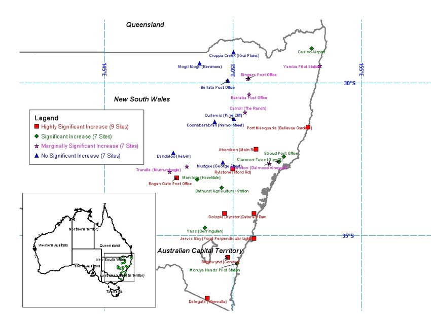
Table 1. Thirty selected stations in southeastern Australia.
  Station                                                                                   Years of              Mean Annual Rainfall (mm)
   No.      Location                                       Longitude       Latitude         Record           1919‐1948    1949‐1978    1979‐2008
  50004     Bogan Gate Post Office                         147° 48′ E      33° 6′ S           103               452          581           462
  50018     Dandaloo (Kelvin)                              147° 40′ E      32° 17′ S          115               436          552           497
  50028     Trundle (Murrumbogie)                          147° 31′ E      32° 54′ S          121               408          549           471
  50031     Peak Hill Post Office                          148° 11′ E      32° 43′ S          116               492          644           568
  52019     Mogil Mogil (Benimora)                         148° 41′ E      29° 21′ S          119               445          536           527
  53003     Bellata Post Office                            149° 48′ E      29° 55′ S           91               529          657           623
  53018     Croppa Creek (Krui Plains)                     150° 1′ E       28° 60′ S           92               517          629           597
  54003     Barraba Post Office                            150° 37′ E      30° 23′ S          125               629          764           685
  54004     Bingara Post Office                            150° 34′ E      29° 52′ S          124               670          771           709
  55045     Curlewis (Pine Cliff)                          150° 2′ E       31° 11′ S          103               505          650           631
  55055     Carroll (The Ranch)                            150° 28′ E      30° 58′ S          112               549          675           602
  58012     Yamba Pilot Station                            153° 22′ E      29° 26′ S          129              1390         1599          1438
  58063     Casino Airport                                 153° 3′ E       28° 53′ S          130              1078         1170          1006
  60026     Port Macquarie (Bellevue Gardens)              152° 55′ E      31° 26′ S          139              1401         1669          1395
  61000     Aberdeen (Main Rd.)                            150° 53′ E      32° 10′ S          107               550          676           516
  61010     Clarence Town (Grey St.)                       151° 47′ E      32° 35′ S          110              1058         1141          1016
  61014     Branxton (Dalwood Vineyard)                    151° 25′ E      32° 38′ S          116               771          900           808
  61071     Stroud Post Office                             151° 58′ E      32° 24′ S          114              1036         1135          1021
  62021     Mudgee (George St.)                            149° 36′ E      32° 36′ S          135               605          755           705
  62026     Rylstone (Ilford Rd.)                          149° 59′ E      32° 48′ S          116               607          724           548
  63005     Bathurst Agricultural Station                  149° 33′ E      33° 26′ S           97               570          723           628
  63032     Golspie (Ayrston)                              149° 40′ E      34° 16′ S          108               663          827           659
  64008     Coonabarabran (Namoi St.)                      149° 16′ E      31° 16′ S          127               640          834           790
  65022     Manildra (Hazeldale)                           148° 35′ E      33° 10′ S          117               624          761           647
  68016     Cataract Dam                                   150° 48′ E      34° 16′ S           99               903         1316           981
  68034     Jervis Bay (Point Perpendicular Lighthouse)    150° 48′ E      35° 6′ S           105              1051         1478          1146
  69006     Bettowynd (Condry)                             149° 47′ E      35° 42′ S          106               732          927           671
  69018     Moruya Heads Pilot Station                     150° 9′ E       35° 55′ S          131               896         1136           943
  70027     Delegate (Weewalla)                            148° 60′ E      37° 3′ S           115               607          686           580
  70028     Yass (Derringullen)                            148° 53′ E      34° 45′ S          105               670          796           670

                      Pr (W W )=
                                       N ww                                      Rainfall changes can be a result of changes to event rain‐
                                                                     (1)
                                   (N dw + N ww )                            fall amount, or the number of rainfall events, or both. In either
                                                                             case, the CLIGEN parameters provide a rich framework for
                                                                             examining the changes to rainfall attributes, e.g., the amount,
                      Pr (W D)=
                                       N dw                                  duration, and frequency of occurrence in relation to changes
                                                                     (2)
                                   (N wd + N dd )                            to rainfall totals.
                                                                                 Changes to CLIGEN parameter values are related to the
   Mean monthly rainfall is the product of the mean wet day                  underlying changes to mean monthly rainfall for the 30 sta‐
rainfall (Pw ) and the number of wet days for the month (Nw ).
                                                                             tions in southeastern Australia. This allows adjustment to
The mean wet day rainfall is one of the input parameters for
                                                                             CLIGEN parameter values to represent historical changes in
CLIGEN, the average number of wet days is related to the                     rainfall in southeastern Australia, and to determine how CLI‐
transition probabilities:
                                                                             GEN parameter values could be changed to simulate climate
                                N d × Pr (W D)
                                                                             change scenarios in this and similar regions in the world.
                Nw =                                                 (3)         To test this adjustment method, changes in mean monthly
                         [1 − Pr(W W)+ Pr(W D)]                              rainfall between period 1 (1919-1948) and period 2
                                                                             (1949-1978) and regression equations for changes in CLI‐
where Nd is the number of days in the month. Therefore,                      GEN parameter values were used to adjust CLIGEN input pa‐
changes in rainfall amount can be effected through changes                   rameter values for period 1 to derive parameter values for
to wet-day rainfall, or transition probabilities, or both.                   period 2. The calculated and the adjusted parameter values
    Alternatively, rainfall total can be regarded as the product             were then used to simulate the climate for periods 1 and 2, re‐
of the number of rainfall events and the average event rain‐                 spectively, with CLIGEN. The simulated rainfall changes be‐
fall. An event is defined in this article as a period of consecu-            tween periods 1 and 2 were then compared with the changes
tive wet days. Rainfall events are separated by at least one dry             based on observed rainfall changes as well as changes in sim-
day. The average event rainfall in terms of CLIGEN parame‐                   ulated rainfall with CLIGEN and calculated parameter val‐
ters is given by:                                                            ues using historical rainfall data for the two periods separate‐
                                                                             ly. All the simulated climates were based on CLIGEN runs of
                                      Pw
                         Pe =                                        (4)     100 years in duration with disparate random seeds for each.
                                1 − Pr(W | W )

Vol. 54(3): 857-867                                                                                                                              859
Figure 1. Location of the 30 stations selected in southeastern Australia.
Table 2. Classification of statistical significance based on the p-value. two showed marginal increases. Increase in rainfall is not sta‐
Criteria Classification tistically significant for just one of the 30 stations (Clarence
p > 0.1 Not significant Town) (figs. 3 and 4).
0.05 < p < 0.1 Marginally significant In contrast, all the stations showed a lower mean annual
0.01 < p < 0.05 Significant rainfall for period 3 in comparison to period 2. Nine of the
p < 0.01 Highly significant 30stations showed highly significant decrease in mean annu‐
al rainfall. The other 21 stations are evenly classified into the
RESULTS three other categories.
TRENDS IN MEAN ANNUAL RAINFALL The largest increase during periods 1 and 2 occurred at the
All the 30 stations had a greater mean annual rainfall in pe‐ Cataract Dam station, showing a 31% increase in mean annu‐
riod 2 (1949-1978) than in period 1 (1919-1948). Converse‐ al rainfall (an average of 903 mm for 1919-1948 and an aver‐
ly, the last period (1979-2008) had lower mean annual age of 1316 mm for 1949-1978). The smallest increase for
rainfall in comparison to that in the second period for all the the same contrasting periods was a 7% increase at mean
stations tested. As an example, figure 2 shows the time series annual rainfall at Clarence Town. For the second pair of con‐
of annual rainfall at Bogan Gate Post Office. It is clear from trasting periods (1949-1978 vs. 1979-2008), Bettowynd
the diagram that rainfall at the site experienced a dramatic in‐ (Condry) showed the highest decrease in mean annual rain‐
crease from the first to the second 30-year period (452 to fall (38%) of the 30 stations examined. The lowest decrease
581mm year-1). This period of increased rainfall is followed of 2% in mean annual rainfall occurred at Mogil Mogil (Beni‐
by an equally dramatic decrease during the last 30 years, with mora).
mean annual rainfall reduced to 462 mm year-1 for Figure 5 shows a comparison of mean annual rainfall be‐
1979-2008, a level that is very similar to that for the first 30 tween the contrasting periods. It is clear that rainfall was con‐
years (1919-1948). sistently higher in period 2 than in both the preceding and
ensuing 30-year periods. A simple regression between mean
Comparing rainfall for period 1 (1918-1948) and period2
(1949-1978) shows that 67% of the stations (20 out of 30) re‐ annual rainfall for the contrasting periods shows that mean
corded a highly significant increase in mean annual rainfall. annual rainfall on average increased by 14% between period
1 (1919-1948) and period 2 (1949-1978) and subsequently
Seven of the 30 stations showed a significant increase, and
decreased by 19% between period 2 and period 3
(1979-2008).
860 TRANSACTIONS OF THE ASABE1200
Annual Rainfall
1000 Average 1919-1948
Average 1949-1978
Average 1979-2008
800
Rainfall (mm)
581 581
600
452 452 462 462
400
200
0
1910 1920 1930 1940 1950 1960 1970 1980 1990 2000 2010 2020
Year
Figure 2. Time series of annual rainfall amount at Bogan Gate Post Office (1919-2008).
Figure 3. Sites of significant increase in mean annual rainfall between 1919-1948 and 1949-1978 in southeastern Australia.
SEASONAL RAINFALL period 2, followed by a decrease in rainfall for the last
Table 3 shows changes to seasonal rainfall between peri‐ 30years (1979-2008) (tables 3 and 4). For some sites in
ods 1 and 2 and between periods 2 and 3. This is a summary southeastern Australia, the seasonal rainfall does not follow
of the sites with different degrees of statistical significance the increasing and decreasing pattern for annual rainfall, es‐
with respect to the changes in annual and seasonal rainfall in pecially for autumn and winter (tables 3 and 4).
southeastern Australia (table 3). For most seasons, and for a Overall, it is clear from table 3 that rainfall increased be‐
majority of the sites tested, seasonal rainfall followed the tween periods 1 and 2 and decreased between periods 2 and
same pattern as annual rainfall, with a significant increase in 3. The increase between periods 1 and 2 was more dramatic
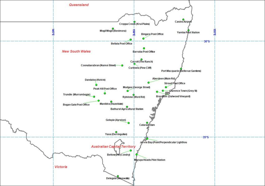
Vol. 54(3): 857-867 861Figure 4. Sites of significant decrease in mean annual rainfall between 1949-1978 and 1979-2008 in southeastern Australia.
2000 2000
(a) (b)
Mean Annual Rainfall, Period 2 (1949-1978)
Mean Annual Rainfall, Period 2 (1949-1978)
1500 1500
1000 1000
500 Highly significant increase Highly significant increase
500
Marginally significant increase Marginally significant increase
Significant increase Significant increase
No significant increase No significant increase
0 0
0 500 1000 1500 2000 0 500 1000 1500 2000
Mean Annual Rainfall, Period 1 (1919-1948) Mean Annual Rainfall, Period 3 (1979-2008)
Figure 5. Comparison of the mean annual rainfall between the three 30-year periods for the 30 stations in southeastern Australia: (a) between
1919-1948 and 1949-1978, and (b) between 1949-1978 and 1979-2008.
and more consistent among the 30 sites tested than the de- CLIGEN PARAMETER VALUES
crease between periods 2 and 3. The increase followed by de‐ Unlike the mean annual rainfall, the mean daily rainfall
crease is most consistent for summer rainfall and least consis‐ for each month does not follow a clear pattern. Daily rainfall
tent for autumn and winter rainfall. In fact, winter rainfall at some of the sites for some of the months increased, and for
experienced no significant increase between periods 1 and 2 others it decreased. The most dramatic increase in mean daily
and no significant decrease between periods 2 and 3 for most rainfall occurred at Cataract Dam, with a 54.9% increase in
of sites tested in southeastern Australia. March (from 1919-1948 to 1949-1978), and the largest de-
862 TRANSACTIONS OF THE ASABETable 3. Variations in rainfall and statistical level of significance: HS = highly significant, S = significant,
MS = marginally significant, NS = not significant, up arrow (°) = increase, and down arrow (±) = decrease.
1919‐1948 to 1949‐1978 1949‐1978 to 1979‐2008
Station Annual Spring Summer Autumn Winter Annual Spring Summer Autumn Winter
Bogan Gate Post Office HS ↑ HS ↑ S↑ S↑ NS ↑ HS ↓ MS ↓ S↓ S↓ NS ↓
Dandaloo HS ↑ S↑ S↑ S↑ NS ↑ NS ↓ MS ↓ MS ↓ NS ↓ NS ↑
Trundle (Murrumbogie) HS ↑ HS ↑ S↑ S↑ NS ↑ MS ↓ NS ↓ MS ↓ NS ↓ NS ↑
Peak Hill Post Office HS ↑ HS ↑ HS ↑ MS ↑ NS ↑ MS ↓ NS ↓ MS ↓ NS ↓ NS ↑
Mogil Mogil (Benimora) S↑ NS ↑ HS ↑ NS ↑ NS ↓ NS ↓ NS ↑ S↓ NS ↑ NS ↑
Bellata Post Office HS ↑ S↑ HS ↑ NS ↑ NS ↓ NS ↓ NS ↑ NS ↓ NS ↓ NS ↑
Croppa Creek (Krui Plains) HS ↑ S↑ HS ↑ NS ↑ NS ↓ NS ↓ NS ↓ MS ↓ NS ↑ NS ↓
Barraba Post Office HS ↑ HS ↑ HS ↑ NS ↑ NS ↓ MS ↓ MS ↓ S↓ NS ↓ NS ↑
Bingara Post Office S↑ MS ↑ HS ↑ NS ↑ NS ↓ MS ↓ NS ↓ NS ↓ NS ↓ NS ↓
Curlewis (Pine Cliff) HS ↑ HS ↑ HS ↑ NS ↑ NS ↓ NS ↓ NS ↓ NS ↓ NS ↑ NS ↑
Carroll (The Ranch) HS ↑ HS ↑ HS ↑ MS ↑ NS ↓ MS ↓ MS ↓ S↓ NS ↑ NS ↑
Yamba Pilot Station S↑ NS ↑ HS ↑ NS ↑ NS ↑ MS ↓ NS ↓ S↓ NS ↑ NS ↓
Casino Airport MS ↑ NS ↑ S↑ NS ↓ NS ↑ S↓ NS ↓ HS ↓ NS ↓ S↓
Port Macquarie S↑ NS ↑ HS ↑ NS ↑ NS ↑ HS ↓ NS ↓ HS ↓ NS ↓ S↓
Aberdeen (Main Rd.) HS ↑ MS ↑ HS ↑ NS ↑ NS ↑ HS ↓ S↓ HS ↓ MS ↓ MS ↓
Clarence Town (Grey St.) NS ↑ NS ↓ S↑ NS ↓ NS ↑ S↓ NS ↑ S↓ NS ↑ S↓
Branxton S↑ NS ↑ HS ↑ NS ↓ NS ↑ MS ↓ NS ↑ S↓ NS ↑ MS ↓
Stroud Post Office MS ↑ NS ↑ HS ↑ NS ↓ NS ↑ S↓ NS ↑ HS ↓ NS ↑ S↓
Mudgee (George St.) HS ↑ S↑ HS ↑ NS ↑ NS ↑ NS ↓ NS ↓ S↓ NS ↓ NS ↑
Rylstone (Ilford Rd.) S↑ NS ↑ HS ↑ NS ↑ NS ↑ HS ↓ MS ↓ HS ↓ S↓ MS ↓
Bathurst Agricultural Station HS ↑ HS ↑ HS ↑ MS ↑ NS ↑ S↓ NS ↓ S↓ MS ↓ NS ↓
Golspie (Ayrston) HS ↑ HS ↑ S↑ MS ↑ NS ↑ HS ↓ MS ↓ HS ↓ S↓ MS ↓
Coonabarabran HS ↑ HS ↑ HS ↑ NS ↑ NS ↓ NS ↓ NS ↓ MS ↓ NS ↑ NS ↑
Manildra (Hazeldale) HS ↑ HS ↑ HS ↑ MS ↑ NS ↑ S↓ NS ↓ S↓ MS ↓ NS ↑
Cataract Dam HS ↑ HS ↑ HS ↑ NS ↑ HS ↑ HS ↓ NS ↓ HS ↓ NS ↓ S↓
Jervis Bay HS ↑ HS ↑ S↑ S↑ HS ↑ HS ↓ HS ↓ HS ↓ S↓ HS ↓
Bettowynd (Condry) HS ↑ HS ↑ NS ↑ NS ↑ S↑ HS ↓ HS ↓ HS ↓ S↓ S↓
Moruya Heads Pilot Station HS ↑ HS ↑ NS ↑ NS ↑ HS ↑ S↓ NS ↓ NS ↓ NS ↓ MS ↓
Delegate (Weewalla) S↑ HS ↑ NS ↓ NS ↑ S↑ HS ↓ S↓ MS ↓ MS ↓ MS ↓
Yass (Derringullen) HS ↑ HS ↑ S↑ MS ↑ NS ↑ S↓ MS ↓ S↓ S↓ NS ↓
Table 4. Direction of change and the statistical level of significance among the 30 sites in southeastern Australia.
1919‐1948 to 1949‐1978 1949‐1978 to 1979‐2008
Directions Annual Spring Summer Autumn Winter Annual Spring Summer Autumn Winter
Increase 30 29 29 26 22 0 5 0 9 11
Decrease 0 1 1 4 8 30 25 30 21 19
Level of significant Annual Spring Summer Autumn Winter Annual Spring Summer Autumn Winter
Highly significant 20 16 19 0 3 9 2 9 0 1
Significant 7 4 8 4 2 7 2 11 6 6
Marginally significant 2 2 0 6 0 7 7 6 4 6
No significant 1 8 3 20 25 7 19 4 20 17
crease occurred at Port Macquarie (Bellevue Gardens), with a probability of wet following dry days. As indicated in table5
108.4% decrease in August (from 1949-1978 to 1979- 2008). and figures 8 and 9, there are no strong correlation between
To determine how CLIGEN parameter values could be changes in mean monthly rainfall and those in skewness and
changed to represent historical trends and patterns in rainfall, wet-following-wet probabilities.
the ratios for five major CLIGEN parameter values between Table 5 presents the R2 values of the linear trend line cor‐
the three contrasting periods for all stations were calculated. relation coefficient squared between the changes in mean
These ratios were then related to the ratios for the mean monthly rainfall and the changes in the five major CLIGEN
monthly rainfall for the same contrasting periods. parameter values. Linear correlation coefficients show that
Figures 6 to 10 show the changes in terms of the ratio of changes in monthly rainfall are closely related changes in
parameter values for the mean, standard deviation, skewness, mean daily rainfall, the standard deviation of daily rainfall,
probabilities of a wet day following a wet day, probabilities and the transition probability for wet following dry days. On
of a wet day following a dry day, and number of wet days for the other hand, the relationship between changes in rainfall
all stations in comparison of the ratio of monthly rainfall for and changes in the skewness coefficient for daily rainfall and
the contrasting periods. Figures 6, 7, and 10 and table 5 show wet-following-wet probabilities is insignificant. To adjust
that there are significant positive correlations between the model parameter values to simulate changes in rainfall,
changes in mean monthly rainfall and changes in mean daily the latter two parameters can remain unchanged based on the
rainfall, standard deviations of mean daily rainfall, and the data for the 30 sites tested.
Vol. 54(3): 857-867 8633.0 3.0
(a) (b)
2.5 2.5
2.0 2.0
MDR2/MDR1
MDR2/MDR3
y = 0.9121x + 0.0604
1.5 1.5 y = 0.8203x + 0.1169
R2 = 0.9107
R2 = 0.8058
1.0 1.0
0.0 0.5 1.0 1.5 2.0 2.5 3.0 0.0 0.5 1.0 1.5 2.0 2.5 3.0
0.5 0.5
0.0 0.0
MMR2/MMR1 MMR2/MMR3
Ratio of MDR2/MDR1 and MMR2/MMR1 Linear (1:1 Line) Linear (Ratio of MDR2/MDR1 and MMR2/MMR1) Ratio of MDR2/MDR3 and MMR2/MMR3 Linear (1:1 Line) Linear (Ratio of MDR2/MDR3 and MMR2/MMR3)
Figure 6. Relationship between changes in mean monthly rainfall (MMR) and changes in mean daily rainfall (MDR): (a) between 1919-1948 and
1949-1978, and (b) between 1949-1978 and 1979-2008.
3.0 3.0
(a) (b)
2.5 2.5
2.0 2.0
MDD2/MDD1
MDD2/MDD3
1.5 1.5
y = 0.6799x + 0.2535
y = 0.7552x + 0.1867
R2 = 0.5942
R2 = 0.6944
1.0 1.0
0.0 0.5 1.0 1.5 2.0 2.5 3.0 0.0 0.5 1.0 1.5 2.0 2.5 3.0
0.5 0.5
0.0 0.0
MMR2/MMR1 MMR2/MMR3
Ratio of MDD2/MDD1 and MMR2/MMR1 Linear (1:1 lINE) Linear (Ratio of MDD2/MDD1 and MMR2/MMR1) Ratio of MDD2/MDD3 and MMR2/MMR3 Linear (1:1 lINE) Linear (Ratio of MDD2/MDD3 and MMR2/MMR3)
Figure 7. Relationship between changes in mean monthly rainfall (MMR) and changes in the standard deviation of mean daily rainfall (MDD): (a) be‐
tween 1919-1948 and 1949-1978, and (b) between 1949-1978 and 1979-2008.
3.0 3.0
(a) (b)
2.5 2.5
2.0 2.0
MDS2/MDS1
MDS2/MSD3
y = -0.0685x + 1.1121
1.5 1.5 R2 = 0.0049
y = 0.0329x + 0.9526
R2 = 0.0015
1.0 1.0
0.0 0.5 1.0 1.5 2.0 2.5 3.0 0.0 0.5 1.0 1.5 2.0 2.5 3.0
0.5 0.5
0.0 0.0
MMR2/MMR1 MMR2/MMR3
Ratio of MDS2/MDS1 and MMR2/MMR1 Linear (1:1 Line) Linear (Ratio of MDS2/MDS1 and MMR2/MMR1) Ratio of MDS2/MDS3 and MMR2/MMR3 Linear (1:1 Line) Linear (Ratio of MDS2/MDS3 and MMR2/MMR3)
Figure 8. Relationship between changes in mean monthly rainfall (MMR) and changes in the Skewness of mean daily rainfall (MDS): (a) between
1919-1948 and 1949-1978, and (b) between 1949-1978 and 1979-2008.
864 TRANSACTIONS OF THE ASABE3.0
3.0 (b)
(a)
2.5
2.5
2.0 2.0
PWW2/PWW3
PWW2/PWW1
1.5 1.5
y = -0.049x + 1.0113
y = 0.1194x + 0.9885 R2 = 0.0044
R2 = 0.0393
1.0 1.0
0.0 0.5 1.0 1.5 2.0 2.5 3.0 0.0 0.5 1.0 1.5 2.0 2.5 3.0
0.5 0.5
0.0 0.0
MMR2/MMR1 MMR2/MMR3
Ratio of PWW2/PWW1 and MMR2/MMR1 Linear (1:1 Line) Linear (Ratio of PWW2/PWW1 and MMR2/MMR1) Ratio of PWW2/PWW3 and MMR2/MMR3 Linear (1:1 Line) Linear (Ratio of PWW2/PWW3 and MMR2/MMR3)
Figure 9. Relationship between changes in mean monthly rainfall (MMR) and changes in the probability of the wet day following a wet day (PWW):
(a) between 1919-1948 and 1949-1978, and (b) between 1949-1978 and 1979-2008.
3.0 3.0
(a) (b)
2.5 2.5
2.0 2.0
PWD2/PWD1
PWD2/PWD3
y = 0.2315x + 0.8385
R2 = 0.1313
1.5 1.5
y = 0.3239x + 0.7344
R2 = 0.3059
1.0 1.0
0.0 0.5 1.0 1.5 2.0 2.5 3.0 0.0 0.5 1.0 1.5 2.0 2.5 3.0
0.5 0.5
0.0 0.0
MMR2/MMR1 MMR2/MMR3
Ratio of PWD2/PWD1 and MMR2/MMR1 Linear (1:1 Line) Linear (Ratio of PWD2/PWD1 and MMR2/MMR1) Ratio of PWD2/PWD3 and MMR2/MMR3 Linear (1:1 Line) Linear (Ratio of PWD2/PWD3 and MMR2/MMR3)
Figure 10. Relationship between changes in mean monthly rainfall (MMR) and changes in the probability of the wet day following a dry day (PWD):
(a) between 1919-1948 and 1949-1978, and (b) between 1949-1978 and 1979-2008.
Table 5. R2 values for linear correlation between changes in mean Table 6. Linear regression equations to predict, from changes in mean
monthly rainfall and changes in CLIGEN parameters for the two monthly rainfall, changes in CLIGEN parameter values of mean daily
contrasting periods and for summer-half and winter-half rainfall, daily standard deviation, and probability of a wet day
of the year (Between 1919-1948 and 1949-1978 periods following a dry day: x = change in monthly rainfall as ratios, and y =
and between 1949-1978 and 1979-2008). changes in model parameter values as ratios (see figures 6, 7, and 10).
Parameter All Months Summer‐Half Winter‐Half Parameter Equation
1919‐1948 and 1949‐1978 1919‐1948 and 1949‐1978
Mean P 0.9107 0.8875 0.9346 Mean P y = 0.9121x + 0.0604
SD P 0.6944 0.6381 0.7503 SD P y = 0.7552x + 0.1867
Skew P 0.0015 0.0000 0.0057 Pr(W | D) y = 0.3239x + 0.7344
Pr(W | W) 0.0393 0.0607 0.0262 1949‐1978 and 1979‐2008
Pr(W | D) 0.3059 0.3106 0.2450 Mean P y = 0.8203x + 0.1169
1949‐1978 and 1979‐2008 SD P y = 0.6799x + 0.2535
Mean P 0.7937 0.7568 0.8206 Pr(W | D) y = 0.2315x + 0.8385
SD P 0.5715 0.5801 0.5542 Combined
Skew P 0.0131 0.0000 0.0496 Mean P y = 0.884x + 0.069, R2 = 0.86
Pr(W | W) 0.0086 0.0063 0.0120 SD P y = 0.729x + 0.208, R2 = 0.66
Pr(W | D) 0.1608 0.2545 0.1117 Pr(W | D) y = 0.287x + 0.776, R2 = 0.22
As mean monthly rainfall is not an input parameter for CLIGEN parameters based on the changes in rainfall that
CLIGEN, some or all the five major parameters for CLIGEN need to be simulated. It is clear that the regression equations
need to be changed to achieve the required change in rainfall. are quite similar whether we consider rainfall increase
Of the five parameters, table 5 shows that there is hardly any (1919-1948 vs. 1949-1978) or rainfall decrease (1978-
correlation between changes in rainfall and changes in skew‐ 2008). A set of regression equations was derived using the
ness and wet-to-wet transition probabilities. Table 6 presents combined data set of data on changes in monthly rainfall and
the linear regression equations that can be used to adjust the changes on CLIGEN parameters (table 6). These equations
Vol. 54(3): 857-867 8651800
1600
1400
Mean Annual Rainfall (mm)
1200
1000
800
600
Observed 1949-1978
400 Calculated 100 years
Adjusted 100 years
Linear (1:1 line)
200
0
0 200 400 600 800 1000 1200 1400 1600 1800
Mean Annual Rainfall (mm)
Figure 11. Mean annual rainfall for 30 selected stations using observed data, calculated and adjusted parameter values (error bars represent the stan‐
dard deviation of the mean).
are recommended for use when mean monthly rainfall can DISCUSSION AND CONCLUSION
vary by a factor of 2.5. Climate change is complex and can have considerable im‐
To test the adjustment method, the combined equations pact on bio‐physical systems and human society. To evaluate
from table 6 were used to adjust the CLIGEN parameter val‐ the impact of climate change, stochastic weather generators
ues for period 1 to estimate the parameter values for period2. are often used to produce daily weather sequences based on
These adjusted parameter values were used to simulate broad‐scale changes predicted by global climate models.
100‐year climate sequences for the 30 sites with CLIGEN. CLIGEN is one such weather generator that has been used for
Calculated parameter values using historical data for peri‐ impact analysis. Unlike other weather generators, CLIGEN
od2 were also used to simulate 100‐year climate sequences produces variables describing storm patterns, including time
for the same 30 sites in southeastern Australia. CLIGEN‐ to peak, peak intensity, and storm duration, in addition to
generated rainfall changes using adjusted and calculated pa‐ rainfall amount and other daily weather variables. While var‐
rameter values were compared with the observed changes ious methods have been proposed to adjust CLIGEN parame‐
between period 1 and 2. The average of the mean annual rain‐ ter values to simulate climate change scenarios, there is little
fall for the 30 sites was 716 mm for period 1 and 875 mm for research on how CLIGEN parameter values could be ad‐
period 2, with an increase of 22%. The average of the mean justed to simulate climate change, whereas previous studies
annual rainfall using calculated parameter values for peri‐ have used simplistic approaches, e.g., changing the average
od2 was 859 mm for the 30 sites, a difference of ‐1.8% of the rainfall on wet days by a percentage or multiplying the
observed average for the 30 sites. Using the parameter values CLIGEN‐generated daily rainfall by a fixed factor.
for period 1 adjusted for changes in mean monthly rainfall be‐ Rainfall in southeastern Australia is highly variable in
tween the two periods led to an average of 890 mm for the time. Instrumental records from the region show significant
30sites, a difference of +1.7% of the observed average for the variability and change on the time scale of climatology,
30 sites. The difference between calculated and adjusted pa‐ i.e.,30 years. These secular changes have been previously
rameter values was 31 mm in terms of the mean annual rain‐ used to indicate the likely rainfall change to represent human‐
fall on average, or 3.5% of the observed average for the induced climate change scenarios. Equally, significant
region. Using paired two‐sample t‐tests for the differences in change in historical rainfall can be used to guide and deter‐
means shows that there is no statistically significant differ‐ mine how parameter values can be adjusted to simulate cli‐
ence in terms of the mean annual rainfall for the 30 sites mate change using stochastic weather generators.
among the three data sets, namely, historical observations This article shows that rainfall data for the period from
and simulated climate with calculated and adjusted parame‐ 1919 to 1978 would suggest an increase in rainfall in south‐
ter values. Figure 11 shows a comparison in the mean annual eastern Australia. However, from the perspective of the peri‐
rainfall between the two contrasting periods. It can seen from od from 1949 to 2008, the conclusion of decreasing rainfall
figure 11 that mean annual rainfall is consistently higher for would be reached. Both of these 60‐year periods broadly
period 2 than for period 1 based on historical observations, coincide with an underlying trend of increased temperature
and using calculated and adjusted parameter values for CLI‐ in Australia and globally (Plummer et al., 1995; IPCC, 2001).
GEN. It is worth noting that the error bars are generally larger Rainfall data from these 30 sites in southeastern Australia
than those for simulated mean annual rainfall because of the shows that we should not draw any conclusions about the
difference in record length. relationship between trends in atmospheric concentration of
greenhouse gases and temperature with regional rainfall.
Rainfall could be just as likely to increase as to decrease sig‐
866 TRANSACTIONS OF THE ASABEnificantly on the time scale of regional climatology (30 years) Nicks, A. D., L. J. Lane, and G. A. Gander. 1995. Chapter 2:
in southeastern Australia. Weather generator. In USDA Water Erosion Prediction Project:
Nonetheless, southeastern Australia provides a rich set‐ Hillslope Profile and Watershed Model Documentation. NSERL
ting to examine how CLIGEN parameter values actually vary Report No. 10. D. C. Flanagan and M. A. Nearing, eds. West
Lafayette, Ind.: USDA‐ARS National Soil Erosion Research
during contrasting wet and dry periods. Daily data for the
Laboratory.
90‐year period for each of the 30 sites in the region show that Pittock, A. B. 1983. Climate change in Australia: Implications for a
there are strong positive correlations between changes in CO2‐warmed earth. Climate Change 5(4): 321‐340.
mean monthly rainfall and changes in mean daily rainfall, Plummer, N., Z. Lin, and S. Torok. 1995. Trends in the diurnal
standard deviation of mean daily rainfall, and the probability temperature range over Australia since 1951. Atmos. Res.
of wet‐following‐dry sequences. There is little evidence to 37(1‐3): 79‐86.
suggest ways of adjusting the skewness coefficient or wet‐ Prudhomme, C., N. Reynard, and S. Crooks. 2002. Downscaling of
following‐wet probabilities to simulate changes in mean global climate models for flood frequency analysis: Where are
monthly rainfall for this region. we now? Hydrol. Proc. 16(6): 1137‐1150.
A set of regression equations was developed to allow easy Pruski, F. F., and M. A. Nearing. 2002a. Runoff and soil loss
responses to changes in precipitation: A computer simulation
adjustment of CLIGEN parameter values (namely, mean dai‐
study. J. Soil Water Cons. 57(1): 7‐16.
ly rainfall amount, standard deviation of daily rainfall, and Pruski, F. F., and M. A. Nearing. 2002b. Climate‐induced changes
probability of wet days following a dry day) to simulate in erosion during the 21st century for eight U.S. locations. Water
monthly rainfall change for both increasing and decreasing Resources Res. 38(12): 1298, doi: 10.1029/2001WR000493.
rainfall change scenarios for southeastern Australia and is po‐ Semenov, M. A., and E. M. Barrow. 1997. Use of a stochastic
tentially applicable in any similar regions in the world. To weather generator in the development of climate change
demonstrate the accuracy and usefulness of these equations, scenarios. Climatic Change 35(4): 397‐414.
CLIGEN parameter values for period 1 were adjusted to sim‐ Wilby, R. L., and T. M. L. Wigley. 1997. Downscaling general
ulate daily rainfall for period 2. Statistical analysis of the ob‐ circulation model output: A review of methods and limitations.
served and simulated mean annual rainfall with calculated Progress in Physical Geography 21(4): 530‐548.
Wilby, R. L., T. M. L. Wigley, D. Conway, P. D. Jones, B. C.
and adjusted parameter values showed that the adjustment
Hewitson, J. Main, and D. S. Wilks. 1998. Statistical
method can be used to reproduce the observed change in rain‐ downscaling of general circulation model output: A comparison
fall, at least in the mean for the 30 sites tested. As this method of methods. Water Resources Res. 34(11): 2995‐3008.
of adjusting CLIGEN parameter values is largely based on an Xu, C. Y. 1999. From GCMs to river flow: A review of
extensive statistical analysis of historical rainfall observa‐ downscaling methods and hydrologic modelling approaches.
tions, it is worth noting that further testing may be required Progress in Physical Geography 23(2): 229‐249.
for other regions of the world, and for simulating significant Yu, B. 1995. Long‐term variation of rainfall erosivity in Sydney.
changes in other aspects of rainfall in addition to the mean. Weather and Climate 15(2): 57‐66.
Yu, B. 2000. Improvement and evaluation of CLIGEN for storm
generation. Trans. ASCE 43(2): 301‐307.
Yu, B. 2005. Adjustment of CLIGEN parameters to generate
REFERENCES precipitation change scenarios in southern Australia. Catena
BoM. 1989. Climate of Australia. Canberra, ACT, Australia: AGPS 61(2‐3): 196‐209.
Press. Yu, B., and D. T. Neil. 1991. Global warming and regional rainfall:
Cornish, P. M. 1977. Changes in seasonal and annual rainfall in The difference between average and high‐intensity rainfalls. Intl.
New South Wales. Search 8: 38‐40. J. Climatol. 11(6): 653‐661.
Favis‐Mortlock, D. T., and M. R. Savabi. 1996. Shifts in rates and Zhang, X. C. 2004. Generating correlative storm variables for
spatial distributions of soil erosion and deposition under climate CLIGEN using a distribution‐free approach. Trans. ASAE 48(2):
change. In Advances in Hillslope Processes, 529‐560. M. G. 567‐575.
Anderson and S. M. Brooks, eds. Chichester, U.K.: Wiley. Zhang, X. C. 2005. Spatial downscaling of global climate model
Goodess, C. M., and J. P. Palutikof. 1998. Development of daily output for site‐specific assessment of crop production and soil
rainfall scenarios for southeast Spain using a circulation‐type erosion. Agric. Forest Meteorol. 135(1‐4): 215‐229.
approach to downscaling. Intl. J. Climatol. 18(10): 1051‐1083. Zhang, X. C. 2007. A comparison of explicit and implicit spatial
IPCC. 2001. Climate Change 2001: The Scientific Basis. downscaling of GCM output for soil erosion and crop
Contribution of Working Group I to the Third Assessment production assessments. Climatic Change 84(3‐4): 337‐363.
Report of the Intergovernmental Panel on Climate Change. J. T. Zhang, X. C., and J. D. Garbrecht. 2003. Evaluation of CLIGEN
Houghton et al., eds. Cambridge, U.K.: Cambridge University precipitation parameters and their implication on WEPP runoff
Press. and erosion prediction. Trans. ASAE 46(2): 311‐320.
Lavery, B. M., A. K. Kariko, and N. Nicholls. 1992. A high‐quality Zhang, X. C., and W. Z. Liu. 2005. Simulating potential response of
historical rainfall data set for Australia. Australian Meteorol. hydrology, soil erosion, and crop productivity to climate change
Magazine 40(1): 33‐39. in Changwu tableland region on the Loess Plateau of China.
Lavery, B. M., G. Joung, and N. Nicholls. 1997. An extended Agric. Forest Meteorol. 131(3‐4): 127‐142.
high‐quality historical rainfall data set for Australia. Australian Zhang, Y. G., M. A. Nearing, X. C. Zhang, Y. Xie, and H. Wei.
Meteorol. Magazine 46(1): 27‐38. 2010. Projected rainfall erosivity changes under climate change
Nicholls, N., and A. Kariko. 1993. East Australian rainfall events: from multimodel and multiscenario projections in northeast
Interannual variations, trends, and relationships with the China. J. Hydrol. 384(1‐2): 97‐106.
Southern Oscillation. J. Climate 6(6): 1141‐1152.
Vol. 54(3): 857-867 867868 TRANSACTIONS OF THE ASABE
You can also read