Using DNA to assess errors in tropical tree identifications: How often are ecologists wrong and when does it matter?
←
→
Page content transcription
If your browser does not render page correctly, please read the page content below
Ecological Monographs, 80(2), 2010, pp. 267–286
! 2010 by the Ecological Society of America

        Using DNA to assess errors in tropical tree identifications:
        How often are ecologists wrong and when does it matter?
                        KYLE G. DEXTER,1,3 TERENCE D. PENNINGTON,2           AND   CLIFFORD W. CUNNINGHAM1
                 1
                     Biology Department, University Program in Genetics and Genomics, Duke University, Box 90338,
                                                 Durham, North Carolina 27708 USA
                              2
                                Royal Botanic Gardens Kew, Richmond, Surrey TW9 3AB United Kingdom

                Abstract. Ecological surveys of tropical tree communities have provided an important
             source of data to study the forces that generate and maintain tropical diversity. Accurate
             species identification is central to these studies. Incorrect lumping or splitting of species will
             distort results, which may in turn affect conclusions. Although ecologists often work with
             taxonomists, they likely make some identification errors. This is because most trees
             encountered in the field are not reproductive and must be identified using vegetative
             characters, while most species descriptions rely on fruit and flower characters. Because every
             tree has DNA, ecological surveys can incorporate molecular approaches to enhance accuracy.
             This study reports an extensive ecological and molecular survey of nearly 4000 trees belonging
             to 55 species in the tree genus Inga (Fabaceae). These trees were sampled in 25 community
             surveys in the southwestern Amazon. In a process of reciprocal illumination, trees were first
             identified to species using vegetative characters, and these identifications were revised using
             phylogenies derived from nuclear and chloroplast DNA sequences.
                We next evaluated the effects of these revised species counts upon analyses often used to
             assess ecological neutral theory. The most common morphological identification errors
             involved incorrectly splitting rare morphological variants of common species and incorrectly
             lumping geographically segregated, morphologically similar species. Total error rates were
             significant (6.8–7.6% of all individuals) and had a measurable impact on ecological analyses.
             The revised identifications increased support for spatially autocorrelated, potentially neutral
             factors in determining community composition. Nevertheless, the general conclusions of
             community-level ecological analyses were robust to misidentifications. Ecological factors, such
             as soil composition, and potentially neutral factors, such as dispersal limitation, both play
             important roles in the assembly of Inga communities. In contrast, species-level analyses of
             neutrality with respect to habitat were strongly impacted by identification errors. Although
             this study found errors in morphological identifications, there was also strong evidence that a
             purely molecular approach to species identification, such as DNA barcoding, would be prone
             to substantial errors. The greatest accuracy in ecological surveys will be obtained through a
             synthesis of traditional, morphological and modern, molecular approaches.
                Key words: biodiversity; DNA barcoding; genealogical species concept; Inga (Fabaceae); Madre de
             Dios, southern Peru; neutral ecological theory; species delimitation; species identification; tropical trees.

                           INTRODUCTION                              ogy of leaves, twigs, bark, and wood) to delimit species.
   In any field-based ecological study, an ecologist must            Yet the paucity of reproductive individuals leads
identify individuals to species. This can be difficult in the        tropical woody plant ecologists to rely on vegetative
species-rich tropics, with many undescribed species and              characters alone for identification. This calls into
often subtle, morphological distinctions between de-                 question the accuracy of species identifications made
scribed species (see Plate 1). Furthermore, in studies of            by tropical ecologists. The corollary to this question is
plants, only a subset of the characters used to describe a           whether inaccurate species identifications are systemat-
species is available for most individuals. Tropical plant            ically biasing the results and conclusions of ecological
taxonomists use both reproductive characters (i.e., the              studies. In this study, we used a procedure of reciprocal
morphology of flowers, fruits, and their associated                  illumination between vegetative morphology and DNA
structures) and vegetative characters (i.e., the morphol-            sequence data to discover and correct mistakes in species
                                                                     identification and delimitation. Then we compare the
   Manuscript received 15 February 2009; revised 28 July 2009;       results of ecological analyses using species identified
accepted 21 September 2009. Corresponding Editor: F. He.             with our method to results using species identified by
   3
     Present address: Laboratoire Evolution et Diversité
Biologique, UMR 5174, CNRS/Université Paul Sabatier,
                                                                     vegetative characters alone.
Bâtiment 4R3, 31062, Toulouse, France.                                 The impact of potentially systematic errors in tropical
   E-mail: kgdexter@gmail.com                                        tree species identification is important because much of
                                                                 267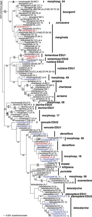
Ecological Monographs
268                                          KYLE G. DEXTER ET AL.
                                                                                                             Vol. 80, No. 2

our current theory and understanding of ecology comes        oxidase I gene commonly used for barcoding animals
from tropical tree communities. One notable example is       (Kress et al. 2005, Newmaster et al. 2006). This increases
the neutral theory of biodiversity and biogeography,         the number of cases in which DNA sequences may not
which was inspired by, and is still largely tested, using    separate closely related species that clearly possess
data from tropical tree communities (Hubbell 1979,           multiple, distinguishing morphological characters. Sec-
2001, Pitman et al. 2001, McGill 2003, Volkov et al.         ond, plants may engage in interspecific gene flow more
2003). Other examples include the intermediate distur-       often than animals (Chase et al. 2005, Cowan et al.
bance hypothesis (Connell 1978, Denslow 1987, Hubbell        2006). Limited past hybridization can obscure patterns
et al. 1999), ecological niche conservatism (Pitman et al.   of species monophyly even when it has not affected
1999, Webb 2000), and the role of density dependence in      species cohesion as determined by morphology (e.g.,
structuring communities (Janzen 1970, Connell 1971,          Quercus; Burger 1975). Nevertheless, when used in
Wills et al. 1997).                                          concert with morphological analyses, DNA sequence
   It is well established that ecologists (Goldstein 1997,   data have the potential to increase the accuracy of plant
Vecchione et al. 2000, Bortolus 2008), including             species delimitation and identification.
tropical tree ecologists (Sheil 1995, Condit 1998), make        As part of a conventional ecological study, we
errors in species identification. Determining how these      surveyed communities of the tropical tree genus Inga
errors affect the results and conclusions of ecological      (Mimosoideae: Fabaceae) at 25 sites across 30 000 km2
studies is more difficult. One must first determine when     of the lowland Amazonian Peru. We encountered nearly
and how many identification errors have occurred. This       4000 individual trees belonging to 63 putative Inga
can be accomplished by having a taxonomic expert             species. As in many ecological studies, individuals were
review all of the ecologists’ identifications (cf. Oliver    first identified using vegetative morphological charac-
and Beattie 1993, Derraik et al. 2002, Scott and Hallam      ters. These identifications were confirmed by careful
2002, Barratt et al. 2003) or through repeated surveys       consultation of herbarium specimens and with the aid of
with different observers (Condit 1998, Archaux et al.
                                                             the recognized taxonomic authority in the genus Inga
2006).
                                                             (co-author T. D. Pennington). Many tropical tree
   Alternatively, genetic data in the form of DNA
                                                             ecology studies incorporate advice from plant taxono-
sequences can be used to assess identification errors
                                                             mists (e.g., Pitman et al. 2001, Phillips et al. 2003,
(Knowlton et al. 1992, Caesar et al. 2006, Bickford et
                                                             Tuomisto et al. 2003), and our morphological identifi-
al. 2007, Stuart and Fritz 2008). For example, the
                                                             cation accuracy should be as good or better than that of
genealogical species concept (Baum and Shaw 1995)
                                                             these other studies.
argues that evolutionarily coherent units can be
                                                                We inferred phylogenies using nuclear and chloro-
identified when gene genealogies reveal monophyletic
                                                             plast DNA sequences for one-quarter of the surveyed
groups of individuals. In practice this means that
                                                             individuals (946 total), encompassing all 63 putative
individuals of a given species should be genetically
                                                             species and multiple locations for widespread species.
more closely related to one another than to individuals
of other species. If a sufficient number of individuals of   We use this phylogeny to propose hypotheses about
the focal species are sequenced for a given gene, then       possible mistakes in species delimitations and identifi-
morphological species can be compared to genealogical        cations. In cases of conflict between this phylogeny and
species to help assess identification accuracy. The large-   the original species designations, we reexamined the
scale sequencing efforts necessary for this type of study    original morphological material and identified three
have previously been considered cost-prohibitive, but        kinds of mistakes: (1) mistakes in individual identifi-
as sequencing costs drop, such studies have entered the      cations; (2) incorrect lumping of morphologically
realm of possibility (e.g., Hebert et al. 2003, 2004,        distinct species; and (3) incorrect splitting of a single
Janzen et al. 2005, Lahaye et al. 2008).                     species.
   Ecologists have long used genetic information to aid         We evaluated the effect of species identification errors
in the identification of individuals (Nanney 1982, Pace      on several analyses that are conventionally used to test
1997, Brown et al. 1999). In fact, in studies of animal      neutral ecological theory (cf. Hubbell 2001). We
taxa, DNA sequence data alone have been used to              conducted analyses that compared the relative impor-
delimit and identify species (termed DNA barcoding;          tance to community assembly of environmental factors,
Hebert et al. 2003, 2004, Janzen et al. 2005). However,      such as soil characteristics, and spatially autocorrelated,
this approach has been criticized because it can fail to     potentially neutral factors, such as dispersal limitation
delimit recently diverged species (Hickerson et al. 2006,    (Duivenvoorden et al. 2002, Legendre et al. 2005,
Knowles and Carstens 2007). There are even fewer             Tuomisto and Ruokolainen 2006). Furthermore, we
reasons to expect a purely genetic approach to be            analyzed distance decay in the compositional similarity
successful in plants.                                        of communities (Condit et al. 2002, Morlon et al. 2008).
   First, most of the genetic markers commonly used for      Finally, we conducted species-level analyses of neutrality
plants, including the ones used in this study, evolve        with respect to habitat preference (Phillips et al. 2003,
much more slowly than the mitochondrial cytochrome           John et al. 2007).
May 2010 ERRORS IN TROPICAL TREE IDENTIFICATION 269
MATERIALS AND METHODS Carolina, USA, for analysis of particle size distribution
Field sites and survey methods (percentage of mass of sand, silt, and clay).
This study focused on distinguishing species within Initial morphological species identification
the genus Inga (Mimosoideae: Fabaceae) (Pennington All surveyed individuals were initially identified to
1997). This is the most diverse and abundant tree genus morphospecies based on vegetative characters. Inga
within the study area of Madre de Dios, in southern species are not highly variable in trunk and bark
Peru (N. Pitman, unpublished data; K. Dexter, personal characters, so we relied largely on leaf characters to
observation). We surveyed Inga communities in the two delimit species. This has the added advantage that
principal habitat types found in the region: terra firme collected vouchers can later be compared with one
(upland) and floodplain (bottomland) forest. another and with identified herbarium specimens. Inga
In community surveys, we first censused all Inga species vary greatly in the number and size of leaflets (all
individuals that reached breast height (1.3 m) in a 50 3 have compound leaves), presence and size of stipules,
50 m plot. If there were fewer than 80 individuals in the presence and nature of pubescence, secondary and
plot, we sampled additional individuals in 2 m wide tertiary venation, the presence and form of wings on
transects until that number was reached (again including the rachis, as well as many other characters, all of which
all Inga individuals that reached breast height). Tran- were used to identify individuals. After vegetative
sects were run in straight lines from the plot and morphospecies were delimited, we reviewed specimens
restricted to the same habitat as the plot (mature from southern Peru in various herbaria to determine
floodplain or terra firme forest). In some locations their taxonomic identity. Representative vouchers of all
(Cocha Cashu, Los Amigos, Las Piedras, Tambopata), species, including unidentified morphospecies, have been
we surveyed Inga individuals in additional 25 3 25 m deposited at Kew Botanic Gardens (K), Duke Univer-
plots. All transects and plots within a given community sity Herbarium (DUKE), and the herbarium of the
survey were restricted to a 2 3 2 km or smaller area. forestry department of La Universidad Agraria La
Within plots or transects, all Inga individuals were Molina in Lima, Peru (MOL).
measured (for diameter at breast height and absolute
height), identified, and collected for a genetic specimen DNA sequences
and, in most cases, an herbarium voucher. When We selected three sets of individuals for verification,
walking trails at study sites, we collected additional via DNA sequencing, of the initial morphological
Inga individuals if they were morphologically unusual identifications. First, we selected ;100 individuals at
and also to boost the sample size of individual species. random from community surveys in floodplain and terra
These additional individuals were not included in firme at our two principal field sites, Cocha Cashu and
community survey totals as they were not randomly Los Amigos (a total of 442 randomly selected individ-
sampled. uals). Second, we sequenced at least two individuals of
For each community survey, we obtained a soil all putative species that were not covered by the above
sample from the 50 3 50 m plot by bulking soil cores sequencing. Third, for most widespread species (I. alata,
taken at five random points throughout the plot. Soil alba, auristellae, bourgonii, cayennensis, chartacea, cin-
samples were also collected from the additional 25 3 25 namomea, edulis, marginata, poeppigiana, ruiziana, sa-
m plots installed at some sites. All soil samples were sent pindoides, thibaudiana, and umbellifera), we sequenced
to the Clemson University Agricultural Services Labo- individuals from additional sites that spanned the
ratory (Clemson, South Carolina, USA) for analyses. breadth of their distribution within the study area. We
Soil pH was measured using an AS-3000 Dual pH also collected and sequenced individuals of the genus
Analyser (LabFit, Perth, Australia). The pH of a buffer Zygia (Mimosoideae: Fabaceae), the likely sister genus
solution was also measured to quantify total acidic to Inga (Jobson and Luckow 2007), for use as an
cations (stored acidity; in milliequivalents per 100 g of outgroup in phylogenetic analyses.
soil). Extractable cations (B, Ca, Cu, K, Mn, Mg, Na, We used a modified cetyltrimethylammonium bro-
Zn) and phosphorous were quantified (in ppm) using the mide (CTAB) protocol (Doyle and Doyle 1990) to
Mehlich 1 procedure. Nitrate nitrogen (NO3!) was extract DNA from silica-gel-dried leaf specimens from
quantified (in ppm) by cadmium reduction using a Flow all selected individuals. We used polymerase chain
Injection FIALab 2500 instrument (FIAlab, Bellevue, reaction (PCR) to amplify one nuclear region, the
Washington, USA). Cation exchange capacity (CEC; in internal transcribed spacers (ITS 1 and 2) and 5.8S gene
milliequivalents per 100 g soil) was calculated as the sum of the nuclear ribosomal DNA, and one chloroplast
of the total acidic cations and base cations (Ca, K, Mg, region, the trnD-trnT intergenic spacer (which spans
and Na; first converted to milliequivalents per 100 g multiple intergenic spacers). We selected the ITS region
soil). The base saturation percentage (BS) was also based on its previously demonstrated variability in the
calculated (in total and separately for K, CA, Mg, and genus (Richardson et al. 2001; K. G. Dexter, unpublished
Na). Furthermore, samples were sent to the North data) and used the following primers for amplification:
Carolina State Soil Services Laboratory, Raleigh, North ITS 4 (White et al. 1990) and ITS 5a (Stanford et al.Ecological Monographs
270 KYLE G. DEXTER ET AL.
Vol. 80, No. 2
2000). We selected the trnD-trnT region because it could differ for the two genetic regions. We ran two
contained the highest number of polymorphic sites independent runs of four Markov chains for 20 million
among multiple chloroplast intergenic regions that were generations with a heating scheme, selected through
initially screened in the genus (Coley et al. 2005; R. T. preliminary analyses, to minimize the average standard
Pennington, unpublished data). We amplified the trnD-T deviation of split frequencies (Temp ¼ 0.15, Swapfreq ¼
region using the following primers: trnH (trnT in 1, Nswaps ¼ 1). Trees were sampled every 1000
Demesure et al. 1995) and trng2 (Oh and Potter 2003). generations. The average standard deviation of split
Reaction conditions were as follows: one cycle of 948C frequencies reached 2% after 11 million generations and
for 2 min; 40 cycles of 948C for 30 s, 528C for 1 min fluctuated around this value thereafter. We discarded
(558C here for trnD-T region), and 728C for 2 min; 1 trees from the first 11 million generations of each run as
cycle of 728C for 7 min. The 25-lL reaction mix the burn-in. As before, we used PAUP beta version 10.4
consisted of 12.3 lL H2O, 5 lL Q reagent (Qiagen, (Swofford 2002) to produce 50% majority rule consensus
Valencia, California, USA), 2.5 lL Taq Buffer, 0.5 lL trees reflecting posterior probabilities for each node.
dNTP mix (10 mmol/L concentration for each nucleo- In addition to the aforementioned preliminary anal-
tide), 1.25 lL primer 1 (10 lmol concentration), 1.25 lL yses for each marker, we conducted full phylogenetic
primer 2 (10 lmol concentration), 1 lL MgCl2, 0.2 lL analyses separately for each partition, ITS and trnD-T,
Taq polymerase, and 1 lL of DNA template. of the concatenated data set.
Cleaned PCR products were sequenced, using the
amplification primers, on an ABI 3730 XL capillary Assessing identification errors and revising
sequencer (Applied Biosystems, Foster City, California, species delimitations
USA). Sequences were assembled using Sequencher We used a two-step process of reciprocal illumination
version 4.5 (Gene Codes, Ann Arbor, Michigan, USA) to assess errors in the initial morphology-based delim-
and manually aligned in MacClade version 4.06 itations and identifications. Potential errors were first
(Maddison and Maddison 2003). identified through examination of the generated molec-
ular phylogenies. We then reviewed the morphology of
Phylogenetic analyses the species involved as well as relevant herbarium
For the ITS and trnD-T regions, Modeltest version material to confirm whether an error had been made.
3.7 (Posada and Crandall 1998) found the same model We classified errors into three categories.
of sequence evolution using the Akaike information 1. Mistakes in individual identifications.—In consider-
criterion (AIC) (general time reversible model with a ing thousands of individuals in sometimes difficult field
proportion of sites invariant and a gamma distribution conditions, some individual trees may be mistakenly
for variable sites, GTR þ I þ G). Preliminary phyloge- identified. These instances were revealed when an
netic analyses indicated few strongly supported topo- accession of a given species was placed phylogenetically
logical differences between the two regions. Therefore, within another species. If the ambiguous individual
we concatenated the two regions for additional phylo- better matched the morphology of the new phylogenetic
genetic analyses. Once concatenated, we used COL- placement, this was considered a simple identification
LAPSE version 1.2 (Posada 2006) to reduce the data set mistake due to human error and not due to the vagaries
to unique sequences. Thus, individuals with identical of species delimitation.
ITS and trnD-T sequences were represented by only one 2. Incorrect lumping of distinct species.—We may also
placeholder in phylogenetic analyses. If individuals of have made errors in species delimitation. For example, if
two or more species were determined to have the same a putative species falls out as two or more divergent
unique sequence, we retained an individual sequence groups in the phylogeny (as opposed to just one
from each species to aid in assessing the monophyly or individual being divergent), this could indicate that
lack thereof of putative species. multiple species were incorrectly lumped together as one
We conducted a maximum-likelihood analysis in species. In these cases, we reexamined the morphology
Garli version 0.96 (Zwickl 2006) with 100 random of vouchers to determine whether there were any
addition sequence replicates. We used the best-fit GTR þ consistently segregating morphological characters be-
G þ I model, allowing Garli to estimate all parameters tween the phylogenetically divergent groups. If any such
while searching for the optimal phylogeny. We also characters were found, the distinguishing characters
conducted a maximum-likelihood bootstrap analysis were noted, and we considered the two groups to be two
with 1000 bootstrap replicates with Garli version 0.96, separate species.
importing bootstrap trees into PAUP* 4.0b10 (Swofford 3. Incorrect splitting of a single species.—If two or
2002) to produce 50% majority rule consensus trees. more putative species were mixed together within a
We also conducted a Bayesian phylogenetic analysis monophyletic group, this could indicate that they
of the concatenated data set, using Mr. Bayes version actually comprise only one species. If close reexamina-
3.1.2 (Ronquist and Huelsenbeck 2003). We used the tion of vouchers found no consistently segregating
GTR þ I þ G model, but we unlinked the partitions so morphological differences between the putative species,
that parameter values and overall rate of substitution we lumped the original species together as one species. IfMay 2010 ERRORS IN TROPICAL TREE IDENTIFICATION 271
the species did possess segregating, morphological 2.0 (Borcard and Legendre 2004). The PCNMs repre-
characters, we continued to treat them as separate sent spatial structure at multiple spatial scales and were
species, despite the inability to distinguish them genet- obtained by a principal components analysis of a
ically. truncated geographic distance matrix of pairwise dis-
Evolutionarily significant units.—When the phylogeny tances between survey sites. The truncation distance
placed an unidentified morphospecies as sister to a represents the minimum scale at which spatial structure
known species in the phylogeny, we reexamined the can be detected in the data. Following the recommen-
morphology of these individuals and also herbarium dations of Borcard and Legendre (2004), we set the
records of the known species across its entire range (not truncation distance at the minimum distance needed to
just in southern Peru as was done in the first pass). This connect all survey sites within a single network (82 km).
review may indicate that the unidentified morphospecies We used a forward selection approach (Blanchet et al.
falls within the morphological limits of the known 2008), separately for the environmental and spatial
species. However, reciprocal monophyly of our samples variables, to determine which variables contributed
of the two putative species indicates that they may be significantly to variation in community composition.
evolving independently. In these cases, we labeled the Only those variables that were significant (at P , 0.05
originally delimited species as two different evolution- with 9999 permutations) were included in variance
arily significant units (ESUs; Moritz 1994) of the same partitioning analyses. Forward selection was conducted
species. When we tabulated error rates, we did so twice, separately for each variance partitioning analysis. We
both lumping ESUs as single species and treating them used the function forward.sel in the packfor package
as distinct species. (Dray 2007) in the R statistical environment (R
Development Core Team 2008) to conduct forward
Ecological analyses selection.
We conducted the following ecological analyses using We used the function varpart in the R package vegan
three sets of species delimitations: (1) the original (Oksanen et al. 2008) to conduct variance partitioning
delimitations based on vegetative morphology; (2) analyses. We adjusted R 2 values for the number of
delimitations revised using the reciprocal illumination sample sites and explanatory variables (Peres-Neto et al.
procedure and treating ESUs as distinct species; and (3) 2006) to give an unbiased estimate of the proportion of
revised delimitations with lumping ESUs of a given variation explained by each component. We evaluated
species together. the significance of the pure environmental and pure
Partitioning variation in community composition.—To spatial fractions using the functions rda and anova.cca
assess the relative importance of environmental factors in the vegan package with 9999 permutations (Oksanen
vs. spatially autocorrelated, potentially neutral factors in et al. 2008).
determining the species composition of communities, we Distance decay in community similarity.—The impor-
used redundancy analysis within a variance partitioning tance of spatially autocorrelated factors, such as
framework (Legendre et al. 2005, Jones et al. 2008). dispersal, in structuring communities has also been
Specifically, we partitioned the variation in a species-by- frequently examined through analyses of distance decay,
site matrix among four additive components: (1) a pure the decline in similarity in species composition of
environmental component; (2) a pure spatial compo- communities with geographic distance (Condit et al.
nent; (3) a combined spatial–environmental component 2002, Morlon et al. 2008). We used partial Mantel tests
(due to the correlated effects of environmental and (cf. Phillips et al. 2003, Tuomisto et al. 2003, Tuomisto
spatial factors); and (4) an unexplained component. and Ruokolainen 2006) to evaluate the relationship
We used two different types of species-by-site matrices between community similarity and geographic distance,
in variance partitioning analyses. The first was a while controlling for environmental variation. Specifi-
presence/absence matrix in which species were repre- cally, we assessed the correlation between a pairwise
sented by a 1 if present in a community survey and a 0 if community similarity matrix (actually evaluated as
absent. The second consisted of the relative abundance dissimilarity matrix) and a geographic distance matrix,
of each species in each community survey. while including a matrix representing environmental
The environmental component was represented by the distance between communities as a covariate. While
natural logarithm of the 21 measured soil variables for partial Mantel tests may not be appropriate for
each community survey site. We used the mean value of partitioning variation in community composition
soil variables for sites from which more than one soil (Legendre et al. 2005, 2008), they can be useful in
sample was collected. As the number of explanatory determining whether there is significant distance decay.
variables compared to the number of sites was already We used the function mantel.partial in the R package
high, we did not attempt to examine polynomial or vegan (Oksanen et al. 2008).
higher order combinations of environmental variables. We analyzed distance decay using both the Jaccard
The variables used to represent spatial autocorrelation and Bray-Curtis indices of community similarity. The
were principal components of neighbor matrices indices were calculated using the program EstimateS
(PCNMs), generated using the program SpaceMaker version 8.00 (Colwell 2006). The Jaccard index usesEcological Monographs
272 KYLE G. DEXTER ET AL.
Vol. 80, No. 2
presence/absence information, while the Bray-Curtis respect to habitat or specialize on terra firme or
index additionally incorporates abundance information. floodplain. We first calculated h, the relative abundance
Both of these indices vary from 0 to 1, with 1 of a given species across the entire data set. This value is
representing maximal community similarity. Partial also the species’ expected relative abundance in flood-
Mantel tests require that all matrices be phrased in plain and terra firme if the species is neutral. For species
terms of distances between communities, so we convert- that we suspected to be floodplain specialists (i.e., that
ed similarity values to dissimilarity values by taking 1 had greater relative abundance in floodplain), we
minus a given similarity index. We constructed two calculated the binomial probability, Bin(YFP j NFP, h),
different matrices of geographic distance between that we found YFP individuals of the species in
communities, one with straight-line geographic distance floodplain habitat given NFP, the total number of
and one with the natural logarithm of geographic individuals sampled in floodplain habitat, and h. This
distances. is equivalent to assaying whether the observed relative
We used data from collected soil samples to measure abundance of the species in floodplain is significantly
the environmental distance between communities. We different from that expected by chance or under
first conducted a principal component analysis (PCA) neutrality, given our sampling effort. We performed a
on all measured soil variables. We then calculated the similar test for suspected terra firme specialists using
Euclidean distance between communities for the first Bin(YTF j NTF, h). If the P value for a given species for
three principal component axes individually and for the selected binomial test was greater than 0.05, then the
their two- and three-dimensional combinations (these species was classified as neutral. Note that these one-
are the only axes that explained .10% of variation in tailed tests are based on first predicting the direction of a
the soil data). Separate environmental distance matri- species habitat specialization.
ces were constructed using each measure of Euclidean If a species is only represented by a few individuals,
distance. For a given community similarity and then statistical power will be lacking to falsify the
geographic distance matrix, we conducted partial hypothesis that the species is neutral with respect to
Mantel tests multiple times, using each possible habitat specificity. We determined the minimum number
environmental distance matrix as a covariate. This of individuals needed to detect whether a hypothetical
allowed us to control for any possible significant species is a habitat specialist if all sampled individuals
environmental variation in evaluating the distance– were found within a single habitat type. We did not
decay relationship. perform binomial tests on species with sample sizes
The intercept and slope of the relationship between below this threshold of detectability.
community similarity and geographic distance are often
interpreted to reflect the level of dispersal limitation in RESULTS
the landscape (Nekola and White 1999, Chave and Field sites and census results
Leigh 2002, Morlon et al. 2008). We estimated these
parameters using simple linear models relating commu- We surveyed communities at 14 locations across
nity similarity to geographic distance (using both Madre de Dios (Fig. 1), separated by a range of spatial
straight-line distances between communities and their distances (from 3 to 250 km apart). At each location, we
logarithm). attempted to survey both terra firme and floodplain
We then assessed whether the distance-decay param- forest. Floodplain forests can vary from swamp to
eter estimates for the original and revised delimitations successional to mature forests (Kalliola et al. 1991,
differed more than expected by chance. We compared Pitman et al. 1999); we attempted to survey communities
the observed difference in parameter estimates between only in mature floodplain forest, as judged by forest
the two delimitations to that between two null sets of stature and the absence of early primary successional
community similarity values. In the first set, we tree species (e.g., Cecropia membrenacea, Ficus insipida,
randomly selected whether each community pair was Cedrela odorata). At three locations (Otorongo, Blan-
represented by the original or revised similarity value, quillo, and Camungo), we could not access terra firme
while the alternate value was assigned to the same pair in forest. There were thus 25 total community surveys, 14
the second set. Across both sets, we preserved the in floodplain forest and 11 in terra firme forest. (See
original geographic distances between each pair of Supplement for species composition data, geographic
communities. This serves to maintain the distance decay coordinates, and soil data for each community survey.)
inherent in the data, while assessing how different the In several community surveys (floodplain at Blan-
distance-decay parameters can be by chance. The quillo, CM2, and Maizal; terra firme at Boca Manu), the
proportion of 999 null replicates with a difference in total number of sampled individuals was less than 80,
parameter estimates greater than that observed in the while in other surveys, the sample size far exceeded 80
real data gives a P value for this one-tailed test. (131 6 13 individuals [mean 6 SE]; range, 46–282
Species-level ecological analyses.—We used a modified individuals). Excluding low- or high-sample-size com-
version of the approach of Phillips et al. (2003) to munities from our community-level analyses had little
determine whether individual species are neutral with effect on the results presented here.May 2010 ERRORS IN TROPICAL TREE IDENTIFICATION 273
FIG. 1. Map of the study area in Madre de
Dios, Peru. Locations of all sites where tree
community surveys were conducted are given:
MZ, Maizal; CC, Cocha Cashu Biological
Station; PK, Pakitza; SV, Salvador; OT, Otoron-
go; BM, Boca Manu; BL, Blanquillo; CA,
Camungo; RF, Refugio; CM, Centro de Moni-
toreo 2; MC, Centro de Monitoreo 3; LA, Los
Amigos Research Center; LP, Las Piedras
Biodiversity Station; TC, Tambopata Research
Center.
Initial morphological species identification The maximum-likelihood trees for the single-locus
phylogenetic analyses, along with maximum-likelihood
Our initial morphological delimitations revealed 63
bootstrap support values and Bayesian posterior prob-
putative species. Our initial examination of herbarium
abilities, are given in Appendices A and B.
specimens from southern Peru allowed us to assign
Assessing identification errors and revising species
taxonomic names to 43 species, while 20 species
delimitations.—Many species that were delimited based
remained as unidentified morphospecies. Our procedure on vegetative morphology formed reciprocally mono-
of reciprocal illumination for revising these initial phyletic groups in the phylogeny (Inga alba, cinnamo-
morphological identifications is described in the follow- mea, cordatoalata, heterophylla, porcata, psittacorum,
ing sections. setosa, suaveolans, tenuistipula, and morphospecies 17,
DNA sequences.—In total, we obtained DNA se- 22, and 54). These species did not require further
quences for 946 Inga individuals (651 for the ITS nuclear assessment of morphology and were considered well-
region and 892 for the trnD-T chloroplast region) from delimited species (marked with letter A in Fig. 2).
all 63 putative species that were encountered during the Mistakes in individual identifications.—Various species
course of this ecological study (see Supplement for (I. alata, chartacea, longipes, ruiziana, sapindoides,
GenBank accession numbers; the master alignment was sertulifera, steinbachii, umbellifera, and morphosp. 58)
deposited in TreeBase). This represents 24.2% of the contained 1–3 sequenced individuals that were divergent
3912 surveyed individuals. The ITS region varied in from the majority of individuals sequenced for their
length from 638 to 668 base pairs (bp), and the total species and that were nested within other species. In all
aligned data set was 671 bp in length. We found no of these cases, a review of vouchers showed that the
evidence that any of the ITS sequences represented divergent individuals had been identified incorrectly
pseudogenes (Alvarez and Wendel 2003). The trnD-T (highlighted in red in Fig. 2). Once these errors were
region varied in length from 1060 to 1100 bp once the corrected, additional species demonstrated reciprocal
ambiguous ends of sequences were trimmed, and the monophyly in the phylogeny (I. alata, marginata, nobilis,
total aligned data set was 1167 bp in length. Alignment ruiziana, umbellifera, and morphospecies 50, 58, 71, and
of all sequences was unambiguous. 75).
Incorrect lumping of distinct species.—Multiple species
Phylogenetic analyses.—The concatenated data set
were found to comprise two divergent groups in the
contained 191 unique sequences, including seven se-
phylogeny. In the cases of Inga auristellae, poeppigiana,
quences found in samples of the outgroup Zygia.
sapindoides, and sertulifera, our detailed reanalysis of
Including individuals that had identical ITS and trnD-
voucher specimens uncovered morphological characters
T sequences but represented putatively distinct species that distinguished the divergent groups (see Table 1). In
boosted the data set for phylogenetic analysis to a total each of these cases, one group corresponded better to
of 222 concatenated sequences. herbarium specimens of the originally designated
The maximum-likelihood tree for the concatenated species. For the first three species, an extensive review
data set is given in Fig. 2. The Bayesian phylogenetic of herbarium specimens demonstrated that the other
analysis (not shown) gave a highly similar topology. The group actually matched lesser-known, rarely collected
percentage of 1000 maximum-likelihood bootstrap species (I. brevipes, barbata, and fosteriana, respectively).
replicates that supported each node (.50%) and the In the case of I. sertulifera, the other group could not be
Bayesian posterior probabilities for each node (.0.5) matched up with any known species and was given the
are shown in Fig. 2. name I. morphospecies 55. These four cases representEcological Monographs
274 KYLE G. DEXTER ET AL.
Vol. 80, No. 2May 2010 ERRORS IN TROPICAL TREE IDENTIFICATION 275
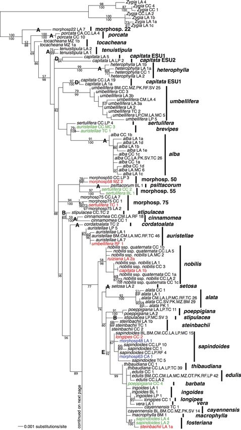
FIG. 2. Maximum-likelihood tree for Inga
samples from Madre de Dios for the concatenat-
ed data set of nuclear internal transcribed spacer
(ITS) and chloroplast trnD-T intergenic spacer
sequences. The percentage of 1000 maximum-
likelihood bootstrap replicates that support a
given node is given above the branch preceding a
node (only given if .50). The posterior proba-
bilities for nodes from a Bayesian phylogenetic
analysis are given below the branches (3100; only
given if .0.5). The taxon labels are followed by
two-letter codes that give the locations at which a
given sequence was found (see Fig. 1) and the
total number of individuals in the molecular
sequence data set with that sequence. The last
lowercase letter provides a unique identifier for
alleles where necessary for comparison with
Appendices A and B. The finalized species
identities are given on the right-hand side of the
tree. The three different categories of error are
color-coded: red indicates mistakes in individual
identification; green indicates incorrectly lumped
species; blue indicates incorrectly split species.
Large boldface letters are referred to in the text
(A, species that were reciprocally monophyletic
under the original delimitations; non-monophy-
letic species pending more information: B, Inga
stipulacea; C, I. morphospecies [morphosp.] 56;
D, I. capitata; E, a speciose clade with little
genetic differentiation between species).Ecological Monographs
276 KYLE G. DEXTER ET AL.
Vol. 80, No. 2
TABLE 1. Morphological characters that were used to delimit incorrectly lumped Inga species as well as characters that can be used
to distinguish the newly segregated species or evolutionarily significant unit (ESU).
Original Segregated Characters used to Characters used to
species species define original species define segregated species
I. auristellae I. brevipes 2–3 pairs leaflets stipules persistent
proximal leaflets basal (short petiole) larger leaflets (3–7 3 6–15 cm
winged rachis flares distally vs. 2–5 3 5–10 cm)
short, orange pubescence on rachis pubescence also on mid-rib of leaflets
narrow stipules
I. poeppigiana I. barbata 3–4 pairs leaflets broader, oblanceolate leaflets
relatively small leaflets (,13 cm long) shorter, narrower stipule (1 mm long,
winged rachis ,0.5 mm wide)
long hispid pubescence (.1.5 mm) brochidodromous venation
I. sapindoides I. fosteriana $3 pairs leaflets denser, more tomentose pubescence
large leaflets (often .25 cm in length) usually $4 pairs leaflets
winged rachis larger, spadiform stipule (1.5–2 3 1–1.5 cm)
orange-red pubescence
regular cup-shaped extra-floral nectary
I. sertulifera I. morphospecies 55 2 pairs leaflets (6–10 3 4–7 cm) narrow, apressed wing on rachis
rounded, elliptical leaflets reticulate tertiary venation
glabrous
narrow stipules
I. capitata I. capitata ESU2 2–3 pairs coriaceous leaflets narrower stipule (,3 mm wide)
glabrous smaller, more elliptic leaflets (3–7 3 7–15 cm
reticulate tertiary venation vs. 4–10 3 10–25 cm)
persistent stipules
I. laurina I. laurina ESU2 2 pairs leaflets (10–16 3 6–12 cm) persistent, short stipules (,1 mm)
rounded, elliptical leaflets
glabrous
sparse, tertiary venation
Note: The study was conducted in Madre de Dios, in southern Peru.
instances of incorrectly lumped species (highlighted in cally (see Table 1). Because capitata LA.LP_2 is
green in Fig. 2). morphologically and genetically distinct from the others,
Inga stipulacea, morphospecies 56, and capitata were it has been designated as a distinct evolutionarily
also polyphyletic in the phylogeny (B–D, respectively, in significant unit (ESU 2). This leaves the other morpho-
Fig. 2). Regarding I. stipulacea, the sampled individuals type polyphyletic pending further information (ESU 1).
strongly resemble one another and are morphologically Inga laurina was found to comprise two well-
very distinct from any other species. The sampled supported sister groups in the phylogeny that, upon
individuals do in fact share a chloroplast allele, but reexamination of vouchers, were found to differ slightly
comprise two divergent clades for the ITS locus. There is morphologically (see Table 1). We therefore split I.
no geographic or morphological segregation of these laurina into two separate ESUs. While other species also
two clades, and we are uncertain of the cause of their comprised sister groups in the phylogeny (e.g., I. alata),
non-monophyly with regards to ITS. We therefore leave these groups were not strongly supported or distin-
the species designation as is, and future research with guishable morphologically.
further nuclear markers may in fact reveal that the Incorrect splitting of single species.—Many species
species does form a cohesive monophyletic clade. were paraphyletic or otherwise phylogenetically inter-
Regarding I. morphospecies 56, it is difficult to say mixed with other species (including multiple cases in
much. The species was only found three times, and in which species shared alleles). In the cases of Inga
fact originally comprised two species (I. morphospecies morphospecies 18, 49, 56, sapindoides, leiocalycina, and
66 was lumped with this species; see Materials and densiflora, a broader review of herbarium specimens
methods: Incorrect splitting of single species). All three showed that other, originally delimited species did not
individuals share the same chloroplast allele, but one possess sufficient segregating morphological characters
individual is divergent for ITS. For now, our conclu- to be distinguished as separate species. These represent
sions regarding this species’ status are very tentative, cases in which we incorrectly split a single species into
and further sampling is needed. multiple species, and we corrected this by lumping the
Inga capitata formed three groups in the phylogeny. species together (highlighted in blue in Fig. 2). In most
All three groups are divergent from one another for the of the cases above, the newly defined species form
ITS marker, while one is divergent from the other two monophyletic clades. However, in the latter two cases (I.
for the trnD-T marker (Appendices A and B). This latter leiocalycina and I. densiflora), the newly delimited
group (capitata LA.LP_2) is also distinct morphologi- species form a paraphyletic grade with respect to otherMay 2010 ERRORS IN TROPICAL TREE IDENTIFICATION 277
TABLE 2. Frequency of different identification and delimitation errors, as assessed through phylogenetic analyses, across an
ecological study of trees in Amazonian Peru.
With ESUs lumped With ESUs treated as species
Total no. Total no. Total no. Total no.
sequenced individuals in sequenced individuals in
Category No. species individuals data set No. species individuals data set
Mistakes in individual ID 10 (15.9%) 16 (1.7%) NA! 10 (15.6%) 16 (1.7%) NA!
Incorrectly lumped 4 (6.3%) 17 (1.8%) 77 (2.0%) 6 (9.4%) 24 (2.6%) 145 (3.7%)
Incorrectly split 12 (19.0%) 31 (3.3%) 83 (2.1%) 9 (14.1%) 32 (3.4%) 126 (3.2%)
Total errors 24 (38.1%) 64 (6.8%) NA! 24 (37.5%) 72 (7.6%) NA!
Total 63 946 3912 64 946 3912
Notes: Values are the number of species or individuals with each type of error. Evolutionarily significant units (ESUs) of a given
species either were lumped together as one species or were treated as separate species-level entities.
! It is not possible to extrapolate the number of mistakes in individual identifications to the entire data set, and thus the total
error rate cannot be calculated for the entire data set.
species, from which they are distinguished by multiple I. venusta and morphospecies 78, although in this case
morphological characters. Inga spectabilis was nested the two ESUs form a paraphyletic grade.
phylogenetically within a paraphyletic I. venusta, and Summary of errors and revisions.—Once the above
based on similar morphology of our vouchers, we errors were taken into account, we revised the identifi-
lumped this species with I. venusta. As the putative I. cations of all 946 sequenced individuals. We then
spectabilis was represented by only one vegetative applied these revisions to the entire ecological data set
accession, it may be premature to take this as signifying of 3912 individuals (see Supplement for revised species
that I. spectabilis is not a good species. composition data). In cases of incorrect lumping, we
Inga nobilis is the only species that we originally used the morphological characters in Table 1 to
delimited to the level of subspecies. Subspecies are determine the identity of unsequenced individuals. In
conceptually similar to ESUs (they should be genetically cases of incorrect splitting, it was straightforward to
and morphologically distinct). In the case of I. nobilis, assign unsequenced individuals of the previously segre-
the two subspecies were intermixed within a monophy- gated species to a single species. Mistakes in individual
letic group. Therefore, we lumped the two subspecies identifications were only detectable through DNA
together as one species, without distinguishing them as sequencing and could not be translated to the entire
separate subspecies or ESUs. data set. The total number and proportion of different
In other cases of potentially incorrect splitting, a types of delimitation and identification errors are given
review of voucher and herbarium specimens demon- in Table 2. The species abundance distribution (SAD)
strated that the originally described species clearly for the original and revised delimitations is given in Fig.
possessed multiple, segregating morphological charac- 3, showing fewer rare species under the revised
ters. This was so for Inga punctata, steinbachii, and delimitations.
tocacheana (paraphyletic with respect to other species),
for several pairs of species that were mixed phylogenet- Ecological analyses
ically (I. bourgonii and coruscans, I. acreana and In presenting the results of ecological analyses, we
chartacea, and I. lineata and killipiana), and in one focus, for the purposes of brevity, on contrasting the
large clade with little genetic divergence between any results using the original delimitations against the
species (E in Fig. 2). In all of these cases, we maintained revised delimitations treating ESUs as distinct species.
the original identifications. The results using the revised delimitations in which
Evolutionarily significant units.—In several pairs of ESUs were lumped as single species were similar to the
species (Inga ruiziana and morphospecies 68, I. tomen- latter and are not presented here.
tosa and morphospecies 71, and I. stenoptera and Partitioning variation in community composition.—
morphospecies 76), the members of the pair fell out as Using presence/absence matrices of species composition,
sister to one another in the phylogeny. Upon extensive the results of variance partitioning analyses differed
review of herbarium vouchers of the named species, it markedly between the original and revised species
was determined that the unnamed morphospecies did delimitations (Table 3); namely, there was an increase
not possess sufficient distinguishing characters to be in the total variation in community composition
separated as distinct species. Thus, these also represent explained. This was due to a large increase in the
cases of incorrectly split species (highlighted in blue in proportion of variation explained purely by spatial
Fig. 2). However, the sister groups are distinct variables (PCNMs). When relative abundance matrices
genetically and somewhat distinct morphologically. We of species composition were used, the original and
therefore labeled these sister groups as distinct ESUs of revised delimitations showed nearly identically results
the nominate species. A similar situation was found for across all analyses.Ecological Monographs
278 KYLE G. DEXTER ET AL.
Vol. 80, No. 2
FIG. 3. The distribution of relative abun-
dances of Inga species across all community
surveys for the original and revised species
delimitations. For the original delimitations,
species that represented incorrect splitting or
lumping are noted. Following convention, a log2
scale is used for the x-axis.
Distance decay in community similarity.—The results similarity, there were also marked differences in
of distance-decay analyses also differed between the estimates of the slope parameter (Table 4, Fig. 4). This
revised and original delimitations (Table 4; see Appen- difference was significant when analyses were restricted
dix C for analyses using log-transformed geographic to terra firme surveys (permutation test, P ¼ 0.012) and
distance). In nearly all cases (except floodplain analyses marginally significant when analyses included all surveys
using the Bray-Curtis index), the revised delimitations (permutation test, P ¼ 0.081). Taken together, these
showed a stronger correlation between geographic results indicate that the revised delimitations give greater
distance and community similarity. When analyses were support to dispersal limitation being an important force
conducted using the Jaccard index of community structuring these communities.
TABLE 3. Results of analyses to partition the variation in composition of Inga communities.
Selected variables! Variance explained (%)
Species delimitation Environmental Spatial Environment Space Environment/space Unexplained
Presence/absence
All sites
Original Ca, B, Na, NO3!, BS_K 1, 13 0.24*** 0.02 0.07 0.67
Revised Ca, B, Na, NO3! 1, 13, 2, 6 0.19*** 0.12** 0.08 0.61
Terra firme
Original Mg, Zn, Mn 1, 5 0.05 0.01 0.2 0.74
Revised Mg, P 1, 5, 3 0.00 0.12* 0.25 0.63
Floodplain
Original B 1, 2 0.00 0.02 0.16 0.82
Revised B 1, 2 0.00 0.03 0.14 0.83
Relative abundances
All sites
Original Ca, Cu, P 1, 13 0.28*** 0.08*** 0.07 0.57
Revised Ca, Cu, P 1, 13 0.27*** 0.08*** 0.08 0.57
Terra firme
Original Mg, Zn 1, 5 0.01 0.11* 0.36 0.52
Revised Mg, Zn 1, 5 0.02 0.12* 0.37 0.49
Floodplain
Original pH 1 0.00 0.00 0.13 0.87
Revised pH 1 0.00 0.00 0.13 0.87
Note: Only the pure environmental and pure spatial fractions can be analyzed for significance, as the other two fractions are
obtained via subtraction.
! These are the variables that were chosen via forward selection for each variance partitioning analysis. They are given in the
order selected. Environmental variables represent soil nutrient concentrations (in the case of named chemicals), pH, or the
percentage base saturation of nutrients (i.e., BS_K). Spatial variables represent spatial autocorrelation via principal components of
neighbor matrices (PCNMs) (see Materials and methods: Partitioning variation in community composition for explanation).
* P , 0.05; ** P , 0.01; *** P , 0.001.May 2010 ERRORS IN TROPICAL TREE IDENTIFICATION 279
TABLE 4. Summary of distance-decay analyses for Inga fera). In three of nine cases in which a species or ESU
communities in Madre de Dios by survey sites included was lumped with another species, the originally segre-
and similarity index.
gated species was classified differently than the species
Species Partial Mantel with which it is now lumped (I. leiocalycina, nobilis, and
delimitation Slope Intercept correlation venusta). Using the revised species delimitations, there
All were fewer rare species in general and therefore fewer
Jaccard cases with too few individuals to detect habitat
Original !2.62 3 10!4 0.363 0.14* specialization (Table 5). For species with sufficient
Revised !3.88 3 10!4 0.388 0.32*** sample size to perform the binomial test, both original
Bray-Curtis and revised delimitations showed the large majority of
Original !1.96 3 10!4 0.295 0.10 species to be habitat specialists (Table 5; 74% for the
Revised !3.36 3 10!4 0.311 0.17** original delimitations vs. 76% for the revised).
Terra firme
Jaccard DISCUSSION
Original !4.38 3 10!4 0.508 0.28* This study represents the first large-scale assessment
Revised !1.08 3 10!3 0.543 0.57**
of the accuracy of vegetative-morphology-based delim-
Bray-Curtis itation and identification of tropical tree species. We
Original !8.05 3 10!4 0.481 0.41**
Revised !9.77 3 10!4 0.481 0.47**
constructed a DNA sequence phylogeny for one-quarter
Floodplain
Jaccard
Original !1.11 3 10!3 0.504 0.40***
Revised !1.05 3 10!3 0.508 0.41***
Bray-Curtis
Original !7.52 3 10!4 0.461 0.27*
Revised !6.66 3 10!4 0.473 0.23*
Notes: The slope and intercept of the relationship between
community similarity and geographic distance were estimated
using a general linear model while the strength and significance
of the relationship were evaluated using partial Mantel tests.
* P , 0.05; ** P , 0.01; *** P , 0.001.
Nevertheless, both the original and revised delimita-
tions did produce similar overall results. Both consis-
tently showed significant distance decay across and
within habitat types and for both community similarity
indices (Table 4, Fig. 4). This result was consistent no
matter which environmental distance matrix was used
as a covariate in the analyses. The results shown in
Table 4 are those in which we constructed the
environmental distance matrix using the Euclidean
distance between communities along the first principal
component axis of all soil variables. The first axis
explained 51% of the variation in the soils data, while
all other axes individually explained at most 15% of the
variation. This environmental distance matrix showed
the strongest relationship with community similarity
matrices, and distance-decay analyses using alternative
environmental distance matrices as covariates showed
the same or even stronger distance decay (results not
shown).
Species-level ecological analyses.—The original and
revised delimitations often differed in how species were
classified with respect to habitat specialization (Appen-
dices D and E). For example, in three of the six cases in FIG. 4. Decline in (upper panel) Jaccard similarity index
which species or ESUs were split based on the reciprocal and (lower panel) Bray-Curtis similarity index with geographic
distance between communities in Madre de Dios for floodplain
illumination procedure, the newly segregated species was
and terra firme Inga communities, showing original and revised
classified differently than the species with which it was species delimitations. Best-fit lines were obtained using a
originally lumped (I. laurina, poeppigiana, and sertuli- general linear model.You can also read