Very Large Array observations of the mini-halo and AGN feedback in the Phoenix cluster
←
→
Page content transcription
If your browser does not render page correctly, please read the page content below
A&A 646, A38 (2021)
https://doi.org/10.1051/0004-6361/202039075                                                                                                               Astronomy
c R. Timmerman et al. 2021                                                                                                                                 &
                                                                                                                                                          Astrophysics

 Very Large Array observations of the mini-halo and AGN feedback
                      in the Phoenix cluster
                     R. Timmerman1 , R. J. van Weeren1 , M. McDonald2 , A. Ignesti3,4 , B. R. McNamara5 ,
                                      J. Hlavacek-Larrondo6 , and H. J. A. Röttgering1

     1
         Leiden Observatory, Leiden University, PO Box 9513, 2300 RA Leiden, The Netherlands
         e-mail: rtimmerman@strw.leidenuniv.nl
     2
         Kavli Institute for Astrophysics and Space Research, Massachusetts Institute of Technology, 77 Massachusetts Avenue, Cambridge,
         MA 02139, USA
     3
         DIFA, University of Bologna, Via Gobetti 93/2, 40129 Bologna, Italy
     4
         IRA INAF, Via Gobetti 101, 40129 Bologna, Italy
     5
         Department of Physics and Astronomy, University of Waterloo, Waterloo, ON, Canada
     6
         Département de Physique, Université de Montréal, C.P. 6128, Succ. Centre-Ville, Montréal, Québec H3C 3J7, Canada

     Received 31 July 2020 / Accepted 10 September 2020

                                                                                     ABSTRACT

     Context. The relaxed cool-core Phoenix cluster (SPT-CL J2344-4243) features an extremely strong cooling flow, as well as a mini
     halo. Strong star formation in the brightest cluster galaxy indicates that active galactic nucleus (AGN) feedback has been unable to
     inhibit this cooling flow.
     Aims. We aim to study the strong cooling flow in the Phoenix cluster by determining the radio properties of the AGN and its lobes. In
     addition, we used spatially resolved radio observations to investigate the origin of the mini halo.
     Methods. We present new multifrequency Very Large Array 1–12 GHz observations of the Phoenix cluster, which resolve the AGN
     and its lobes in all four frequency bands as well as the mini-halo in the L and S bands.
     Results. Using our L-band observations, we measure the total flux density of the radio lobes at 1.5 GHz to be 7.6±0.8 mJy, and the flux
     density of the mini halo to be 8.5 ± 0.9 mJy. Using high-resolution images in the L and X bands, we produced the first spectral index
     maps of the lobes from the AGN and find the spectral indices of the northern and southern lobes to be −1.35 ± 0.07 and −1.30 ± 0.12,
     respectively. Similarly, using L- and S -band data, we mapped the spectral index of the mini halo, and obtain an integrated spectral
     index of α = −0.95 ± 0.10.
     Conclusions. We find that the mini halo is most likely formed by turbulent re-acceleration powered by sloshing in the cool core due
     to a recent merger. In addition, we find that the feedback in the Phoenix cluster is consistent with the picture that stronger cooling
     flows are to be expected for massive clusters such as this one, as these may feature an underweight supermassive black hole due to
     their merging history. Strong time variability of the AGN on Myr timescales may help explain the disconnection between the radio
     and the X-ray properties of the system. Finally, a small amount of jet precession of the AGN likely contributes to the relatively low
     intracluster medium re-heating efficiency of the mechanical feedback.
     Key words. large-scale structure of Universe – radio continuum: galaxies – X-rays: galaxies: clusters –
     radiation mechanisms: non-thermal – galaxies: clusters: individual: SPT-CL J2344-4243

1. Introduction                                                                                  down (e.g., Brüggen & Kaiser 2002; McNamara & Nulsen 2007;
                                                                                                 Fabian 2012).
The emission of strong X-ray radiation by the intracluster
medium (ICM) in galaxy clusters suggests that this medium                                            Studying this feedback process is essential to our under-
should often cool down rapidly: within a timescale of ∼109 years                                 standing of the formation and evolution of galaxies, as it plays
or fewer (e.g., Fabian 1994). As the ICM cools down, it is                                       a critical role in the cooling of the ICM and the star formation
expected to flow down the gravitational well of the cluster, and                                 in galaxies across cosmic time (e.g., Matteo et al. 2005; Croton
accrete onto the galaxy at the center. This accretion of mat-                                    et al. 2006; Menci et al. 2006; Sijacki et al. 2007; Lagos et al.
ter should then trigger star formation in the central galaxies                                   2008; Ciotti et al. 2010; Mathews & Guo 2011; Vogelsberger
proportionally to the cooling flow of the ICM. However, both                                     et al. 2014; Rasia et al. 2015). In particular, clusters of galax-
this cooling of the ICM and the star formation in the center                                     ies form a great opportunity to study AGN feedback, due to the
of the cluster are observed to be much weaker than expected                                      relatively dense ICM, which is capable of creating strong cool-
(Fabian et al. 1982; McNamara & O’Connell 1989; Page et al.                                      ing flows. The ICM is often also dense enough to keep the jetted
2012; McDonald et al. 2018), leading to what is known as the                                     outflows from the AGN contained, which allows this mechanical
“cooling flow problem”. The generally accepted solution to this                                  form of feedback to be studied in detail (McNamara & Nulsen
problem is that feedback from active galactic nuclei (AGN) sup-                                  2012).
plies energy to the ICM in the form of radiation and jetted out-                                     The interaction between the ICM and the jetted outflows
flows of plasma, thereby preventing the medium from cooling                                      from the AGN can be directly observed in the X-ray regime.
                                                                                                                                                                             A38, page 1 of 12

                Open Access article, published by EDP Sciences, under the terms of the Creative Commons Attribution License (https://creativecommons.org/licenses/by/4.0),
                                 which permits unrestricted use, distribution, and reproduction in any medium, provided the original work is properly cited.
A&A 646, A38 (2021)

As the jetted outflows displace the ICM, they create large            2. The Phoenix cluster
cavities that are observed as depressions in X-ray observations.
At radio frequencies, bubbles of synchrotron-emitting plasma          In this work, we focus on the Phoenix cluster (SPT-CL J2344-
are observed to be coincident with these cavities, verifying that     4243), a massive galaxy cluster at redshift z = 0.597 discovered
these cavities are produced by the AGN (Gull & Northover 1973;        by Williamson et al. (2011) in the 2500 deg2 South Pole Tele-
Gitti et al. 2012).                                                   scope Survey. The Phoenix cluster is a relaxed cool-core cluster
     Despite much research into AGN feedback in galaxy clus-          featuring a type 2 QSO (Ueda et al. 2013), and it is characterized
ters, many open questions remain. Of particular interest for this     by its high cooling flow and star formation rate (Kitayama et al.
work is the connection between the central AGN and the mini           2020). X-ray, optical, and infrared observations by McDonald
halo surrounding the brightest cluster galaxy (BCG). Mini halos       et al. (2012, 2013, 2019) show a cooling flow of ∼3100 M per
are faint, diffuse synchrotron-emission regions commonly found        year, with a star-formation rate of ∼800 M yr−1 . Whereas the
in relaxed cool-core galaxy clusters. They span a region of a         star formation rate is generally on the order of 1% of the pre-
few hundred kpc, as they are generally confined to the cool-core      dicted cooling flow, for the Phoenix cluster this ratio is almost
region of a galaxy cluster. Mini halos often feature an amorphous     30%, indicating that the feedback process has not been able to
shape, and have been found to show steep spectral indices of          completely inhibit the cooling flow. Spectroscopic observations
around α = −1 to α = −1.5 (Gitti et al. 2004; Giacintucci et al.      of the warm and cold gas in the core of the Phoenix cluster sug-
2019; Van Weeren et al. 2019).                                        gest that this rapid star formation may be a short phase, as the
     The origin of mini halos remains a topic of debate, which is     molecular gas supply is expected to deplete on a timescale of
hampered by the difficulty of obtaining high-quality data on mini     ∼30 Myr (McDonald et al. 2014).
halos, as the central AGN often dominates the view. The emis-              Using Chandra observations, Hlavacek-Larrondo et al.
sion of synchrotron radiation in the mini halo means that there       (2014) revealed the presence of X-ray cavities in the ICM.
must be a population of cosmic-ray electrons present in a mag-        Follow-up research using deeper observations by McDonald
netic field. However, based on the short lifetime of these elec-      et al. (2015, 2019) provided an estimate of the scale of these cav-
trons of 10–100 Myr, they must be accelerated in-situ (Brunetti       ities of 8–14 kpc, which suggests a jet power from the AGN of
& Jones 2014). Two mechanisms are proposed by which the               1.0+1.5      46     −1
                                                                          −0.4 × 10 erg s . In addition, star-forming filaments extend-
electrons can be accelerated. In the hadronic model, relativis-       ing up to 50–100 kpc from the core of the cluster were observed
tic, secondary electrons are injected by collisions between rel-      using deep optical imaging. ALMA observations also show
ativistic and thermal protons (e.g., Pfrommer & Enßlin 2004;          molecular gas filaments measuring 10–20 kpc in length tracing
Fujita et al. 2007). This model predicts the presence of diffuse      the edges of the X-ray cavities (Russell et al. 2017).
gamma-ray emission, produced by the same proton-proton col-                Observations using the Giant Metrewave Radio Telescope
lisions and a gradual decrease in radio emission due to the diffu-    (GMRT) by Van Weeren et al. (2014) uncovered a mini halo
sion of cosmic ray (CR) protons in the ICM. In the case of radio      surrounding the BCG, which spans a region of 400–500 kpc.
emission produced purely by secondary electrons, the spectral         This mini halo was later observed by Raja et al. (2020) using the
index would depend only on the energy distribution of the CR          Karl G. Jansky Very Large Array (VLA) in CnB configuration.
protons, and hence it would not vary with the radius.                 By subtracting compact emission from their data, they detect the
     Alternatively, according to the turbulent re-acceleration        mini halo and derive a flux density of the mini halo at 1.5 GHz
model, fossil electrons from the AGN are re-accelerated to high       of 9.65 ± 0.97 mJy. They find that the 3σ contours of their map
energies by magneto-hydrodynamic turbulence in the cluster            span a region of 310 kpc.
(e.g., Gitti et al. 2002; Mazzotta & Giacintucci 2008; ZuHone              New deep Chandra and X-band VLA observations by
                                                                      McDonald et al. (2019) revealed radio jets that are coincident
et al. 2013). This turbulence is thought to generally be caused
                                                                      with the previously detected X-ray cavities. In addition, they
by strong cooling flows or a merger event in the recent his-
                                                                      present Hubble observations suggesting that the AGN may lift
tory of the cluster, although recent observations of an Mpc-
                                                                      cool low-entropy gas up to larger radii, where it can cool faster
scale radio halo in a cool core cluster (Bonafede et al. 2014)
                                                                      than its fallback time, resulting in multiphase condensation. The
and ultra-steep-spectrum emission extending beyond the cool
                                                                      gas kinematics and strong high-ionization emission lines indi-
core (Savini et al. 2018) have challenged that idea. The tur-
                                                                      cate that relatively strong turbulence may be present in the core.
bulent re-acceleration model predicts a possible steepening of
                                                                           In this paper, we aim to investigate the strong cooling flow
the spectrum with radius and a radio brightness profile that is
                                                                      observed in the Phoenix cluster by imaging the AGN and its jet-
strongly contained by the cold fronts produced in the ICM by
                                                                      ted outflows across a wide range of radio frequencies. In addi-
a recent merger event. These cold fronts are density disconti-
                                                                      tion, we aim to study the origin of the mini halo by measuring
nuities created by the cold and dense gas from the cool core
                                                                      its properties using spatially resolved radio observations for the
or a subcluster moving through the surrounding hot gas, and
                                                                      first time.
therefore they also commonly form the boundary of a turbulent
region (e.g., Markevitch & Vikhlinin 2007). Accurately deter-
mining the properties of mini halos is essential to understand-
                                                                      3. Observations and data reduction
ing the underlying acceleration mechanism, and thereby their
origin.                                                               The Phoenix cluster was observed with the VLA in the L, S , C,
     In this paper, we adopt a ΛCDM cosmology, with cosmo-            and X bands, covering the frequency range from 1 GHz to
logical parameters of H0 = 70 km s−1 Mpc−1 , Ωm = 0.3, and            12 GHz (PI: McDonald, 17A-258). The X-band data of this
ΩΛ = 0.7. In this cosmology, the luminosity distance to the           project was previously presented by McDonald et al. (2019). In
Phoenix cluster at z = 0.597 is 3508 Mpc, and an angular              the L band, the VLA observed in both A and B configuration,
scale of 1 arcsecond at this redshift corresponds to 6.67 kpc. Fur-   which we complement with archival CnB-configuration obser-
thermore, we followed the convention of defining our spectral         vations (PI: Datta, 14B-397) recently presented by Raja et al.
indices according to S ∝ να .                                         (2020). In the S , C, and X bands, the VLA observed in A, B, and
A38, page 2 of 12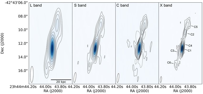
R. Timmerman et al.: VLA observations of the mini-halo and AGN feedback in the Phoenix cluster

Table 1. Summary of the observations.                                     the AOFlagger software (Offringa et al. 2010) was used to
                                                                          remove any remaining RFI.
   Configuration          Obs. date       Freq.   Int. time    θFWHM           Finally, we improved the calibration through the process of
                                         (GHz)       (s)         (00 )    self-calibration. We used CASA to calculate new calibration
                                                                          solutions and applied these to the data, and we used WSClean
   L-band, A-array      24 Mar. 2018       1–2       2        3 × 0.7     (Offringa et al. 2014) for the imaging and deconvolution. Each
   L-band, B-array      2 Nov. 2017        1–2       3        10 × 2      data set was self-calibrated by initially performing phase-only
   L-band, CnB-array    23 Jan. 2015       1–2       5        16 × 9      self-calibration, and later performing amplitude and phase self-
                                (archival)
                                                                          calibration, with iteratively shorter calibration solutions. Then,
   S -band, A-array     11 Mar. 2018       2–4       2         2 × 0.4
                                                                          all data sets of the same spectral band were concatenated to form
   S -band, B-array     25 Sep. 2017       2–4       3          6×1
                                                                          one data set per band. These data sets were then self-calibrated
   S -band, C-array     10 Jun. 2017       2–4       5         18 × 4
                                                                          again to obtain the final data sets. Imaging was performed using
   C-band, A-array       4 Mar. 2018       4–8       2         1 × 0.3
   C-band, B-array       8 Sep. 2017       4–8       3         3 × 0.6
                                                                          Briggs weighting (Briggs 1995) with a robust parameter of zero.
   C-band, C-array       9 Jun. 2017       4–8       5          9×2
                                                                          The C-band data experienced issues during calibration, which is
   X-band, A-array       6 Mar. 2018       8–12      2        0.5 × 0.1   suspected to be caused by the very low declination of the source.
   X-band, B-array       7 Sep. 2017       8–12      3         2 × 0.4    For this reason, it is difficult to discern real structures from noise
   X-band, C-array       5 Jun. 2017       8–12      3          6×1       features near the AGN.

                                                                          4. Results
                                                                          The images we obtain are shown in Fig. 1. The L-band image
C configuration. The L- and S -band observations were recorded            shows the central compact AGN with the diffuse mini halo sur-
using 16 spectral windows of 64 channels each, resulting in a             rounding it. The mini halo is less visible in the S -band image
total bandwidth of 1 GHz and 2 GHz, respectively. The C- and              due to its spectral slope, as well as the more compact beam.
X-band observations were recorded using 32 spectral windows               In the C-band image, the jetted outflows are visible toward the
of 64 channels each, resulting in a total bandwidth of 4 GHz for          north and the south of the AGN. A small part of the mini halo
both bands. All new observations have a total of 2.5 hours of             is still visible toward the east and west of the AGN. Finally, the
integration time per configuration. An overview of the observa-           X-band image shows the jets at the highest angular resolution.
tions is presented in Table 1.                                            The total flux densities, peak fluxes, root mean square (rms)
    For our new observations, we used 3C138 and 3C147 as pri-             noise levels, and beam sizes of the final images are summarized
mary calibrators with a total integration time of approximately           in Table 2.
five to ten minutes at the end of the observation. As the sec-                 To show the maximum resolution attainable with each of the
ondary calibrator, we used J0012-3954. Scans with an integra-             four data sets, images of the target using lower robust parameters
tion time of approximately two to three minutes on the secondary          are shown in Fig. 2. This shows that using a different weight-
calibrator were repeated every 15 min. In the archival L band,            ing scheme, the jetted outflows can even be resolved in the L
CnB-array data, 3C48 was observed for 12 min as the primary               band. Comparing our observations to the ATCA observations of
calibrator. No secondary calibrator was included in this observa-         Akahori et al. (2020), we find that our VLA observations are
tion.                                                                     able to resolve all components observed with the ATCA: C1
    The data were reduced with the Common Astronomy Soft-                 (AGN core), C2, C4, C5 (northern lobe), and C3 and C6 (south-
ware Application (CASA; McMullin et al. 2007). The data                   ern lobe). Akahori et al. (2020) mention that they possibly detect
reduction begins with a Hanning smoothing, the flagging of                jet precession, as components C3 and C4 (near the AGN), appear
shadowed antennas, the calculation of gain elevation curves and           to be emitted in a different direction than components C2 and C6
corrections to the antenna positions, and the use of the TFCrop           in the northern and southern jets, respectively.
algorithm within CASA to apply automatic radio frequency                       The emission from the AGN appears to be coincident with
interference (RFI) flagging. Next, manual flags were applied to           the BCG, as shown in Fig. 3. In addition, the L-band emission
exclude bad data from the calibration process. After the flag-            extends far beyond the optical size of the BCG and the star-
ging, the initial complex gain solutions were calculated based            forming filaments. The radio emission from the cluster coin-
on the central channels from each spectral window. These initial          cides with X-ray emission detected by Chandra (McDonald
complex gain solutions were used to determine the delay terms.            et al. 2015), as shown in Fig. 4. To confirm that the jetted out-
The bandpass calibration solutions were then derived based on             flows detected in our VLA observations are coincident with
the delay terms and the initial complex gain solutions. With the          the cavities previously detected in the ICM, we subtracted a
correct bandpass solutions applied, the complex gain solutions            β-model from the X-ray map, and then overlaid the L- and X-
can be derived for the complete bandwidth of each spectral win-           band contours on the residuals, as shown in Fig. 5. Although
dow. Using the polarized calibrator 3C138, we derived the global          there is a small subarcsecond uncertainty in the relative align-
cross-hand delay solutions. The unpolarized calibrator, 3C147,            ment between the images, it is clear that the X-ray cavities are
then allowed the polarization leakage terms to be calculated.             inflated by magnetized radio plasma. We find no radio emission
Finally, 3C138 was used again to calibrate the polarization angle.        coincident with the possible ghost cavities previously marginally
Using all relevant calibration tables, the complex gain solutions         detected by McDonald et al. (2015) farther toward the north-east
were redetermined, and the flux scale was set based on mod-               and south-east.
els of 3C138 and 3C147 by Perley & Butler (2013). The cal-                     To derive the overall spectral index of the source, we com-
ibration solutions were then applied to the target source, after          bined measurements of the total flux density of the cluster
which the TFCrop and RFlag automatic flagging algorithms                  in our four bands with archival data from Mauch et al. (2003),
were used to remove previously undetected RFI. Next, the cali-            McDonald et al. (2014), Van Weeren et al. (2014) and Akahori
brated data of the target source were split out, after which point        et al. (2020). We assume a 5% uncertainty on our flux density

                                                                                                                              A38, page 3 of 12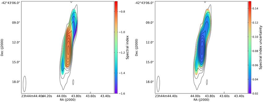
A&A 646, A38 (2021)

Fig. 1. VLA images of Phoenix cluster in L band (top-left), S band (top-right), C band (bottom-left), and X band (bottom-right). Contours are
drawn at [−1, 1, 2, 4, 8, ...] × 4σrms , where σrms = 10.8 µJy beam−1 (L band), σrms = 5.9 µJy beam−1 (S band), σrms = 4.3 µJy beam−1 (C band), and
σrms = 2.2 µJy beam−1 (X band). The beam sizes are indicated in the bottom-left corners of each panel.

Table 2. Properties of the images shown in Fig. 1.

                         Freq. band     Flux density        Peak flux          rms noise        bmajor   bminor     bPA
                                           (mJy)          (mJy beam−1 )      (µ Jy beam−1 )      (00 )    (00 )    (deg)
                         L-band              33.8              20.4               10.8            5.1      1.1     −3.7
                         S -band             18.0              10.5               5.9             3.4     0.74     −8.6
                         C-band              7.95              6.46               4.3             2.5     0.51     −5.9
                         X-band              4.01              3.20               2.2            0.96     0.22     −5.6

estimates in accordance with Perley & Butler (2017). By fit-               term to be consistent with zero within the 95% confidence inter-
ting a power-law profile through the data, we obtain an overall            val. We excluded the data point at 220 GHz from this fit, as we
spectral index of −1.12 ± 0.02, as shown in Fig. 6. To account             expect that free-free and thermal dust emissions can significantly
for a possible curvature in the spectrum, we fit a second-degree           contribute to the spectrum at such high frequencies, causing the
polynomial in log-space through the data, but find the curvature           model of a single power law to break down.

A38, page 4 of 12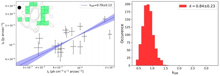
R. Timmerman et al.: VLA observations of the mini-halo and AGN feedback in the Phoenix cluster

Fig. 2. VLA images of Phoenix cluster in L band (robust −1.5), S band (robust −1), C band (robust −0.5), and X band (robust 0). Contours are
drawn at [−1, 1, 2, 4, 8, ...] × 4σrms , where σrms = 40.8 µJy beam−1 (L band), σrms = 12.8 µJy beam−1 (S band), σrms = 6.9 µJy beam−1 (C band),
and σrms = 2.2 µJy beam−1 (X band). The source components as detected by Akahori et al. (2020) using the ATCA are indicated in the X-band
map. The beam sizes are indicated in the bottom-left corners of each panel.

                                                                               Fig. 4. X-ray (0.7–2 keV) image by Chandra (McDonald et al. 2015).
Fig. 3. Optical r-band image of Phoenix cluster taken with Megacam on          The white contours indicate the L-band emission as observed with the
the Magellan Clay Telescope (McDonald et al. 2015). The red contours           Very Large Array and are drawn at [−1, 1, 2, 4, 8, ...] × 4σrms , where
indicate the X-band emission and are drawn at [−1, 1, 2, 4, 8, ...]× 4σrms ,   σrms = 10.8 µJy beam−1 .
where σrms = 2.2 µJy beam−1 .

                                                                               the total flux density of 33.8 mJy, we find that there is a discrep-
    To study the mini halo and the AGN, we needed to separate                  ancy of 8.6 mJy, which we attribute to the mini halo.
these two components. By producing a map of the source using                       Alternatively, the flux density of the mini halo can be esti-
only the long baselines, we obtained an image of the AGN and its               mated through radial profile fitting by describing both the AGN
jets, without contamination from the more extended mini halo.                  and the mini halo using circular Gaussians. This enables the
Based on the X-band imaging, we find that the AGN and its jets                 flux of the AGN and the mini halo to be spatially disentangled,
are more compact than an angular scale of ten arcseconds, which                thereby potentially providing a more accurate measurement of
corresponds to a limit on the baseline length of 20 kλ. After hav-             their total flux densities. We produced an L-band image with
ing produced an L-band image using only baselines longer than                  a Briggs robust parameter of −1 to improve the resolution of
20 kλ, we find that the remaining flux density of the source is                the image, and thereby reduced the scale of the central AGN.
25.2 mJy within the 3σ contours. Comparing this flux density to                This image was smoothed to a circular beam of 2.8 arcseconds
                                                                                                                                    A38, page 5 of 12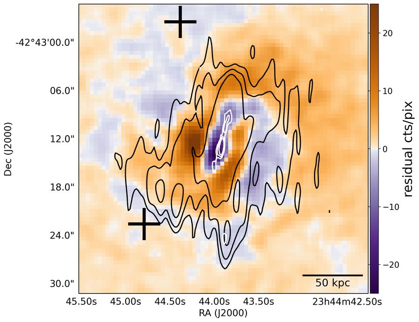
A&A 646, A38 (2021)

                                                                              The estimate obtained with a mask for the flux density of the
                                                                              mini-halo is considerably lower, at only 5.9 mJy. As the values
                                                                              obtained from the first two methods agree very well, we adopt a
                                                                              value of 8.5 mJy for the flux density of the mini halo in L band
                                                                              for the rest of this paper.
                                                                                  From the radial fitting process, we can also obtain an esti-
                                                                              mate for the extent of the mini halo. From the radial fit, we
                                                                              find that it can be described by a Gaussian with a FWHM of
                                                                              13.8 arcseconds, deconvolved with the beam. At a redshift of
                                                                              z = 0.597, this corresponds to a scale of 92 kpc. The maxi-
                                                                              mum observable radius of the mini halo – defined as the radius at
                                                                              which the mini halo reaches the noise level – is 17.8 arseconds,
                                                                              or about 120 kpc. This gives a total diameter of the mini halo of
                                                                              ∼240 kpc.
                                                                                  To map the spectral index of the halo, we smoothed both the
                                                                              L-band and the S -band images to a circular beam size of five
                                                                              arcseconds and aligned the images by matching the positions of
Fig. 5. Residuals of Chandra X-ray image (McDonald et al. 2015)               a nearby point source. To avoid contamination from the AGN
minus a β-model. The residuals were smoothed by a boxcar function             and its jets, we masked out the central region using the same
with a scale of three pixels (1.5 arcsec). The white contours indicate        mask as with the radial fitting. After calculating the spectral
the emission in the X band as observed with the VLA and are drawn at          index between the two maps and excluding the masked region,
[−1, 1, 4, 16] × 4σrms , where σrms = 2.2 µJy beam−1 . The black contours     we obtained the spectral index map of the mini halo as shown in
indicate the emission in the L band as observed with the VLA, and are         Fig. 7.
drawn at [−1, 1, 2, 4] × 4σrms , where σrms = 10.8 µJy beam−1 . The black         The spectral index map of the mini halo shows an annu-
pluses indicate the positions of the ghost cavities detected by McDonald      lus with a mean spectral index of α = −0.95 ± 0.10. However,
et al. (2015).                                                                the signal-to-noise ratio is too low to provide insight about any
                                                                              potential gradients or cut-offs in the spectrum as a function of
                                                                              radius. Using this spectral index, we calculated the radio lumi-
                                                                              nosity of the mini halo using
                                                                              P1.4 GHz = 4πS 1.4 GHz D2L (1 + z)−α−1 ,                       (1)
                                                                              where S 1.4 GHz is the flux density at 1.4 GHz and DL is the lumi-
                                                                              nosity distance to the source, and we find a value of P1.4 GHz =
                                                                              (13.0 ± 1.4) × 1024 W Hz−1 .
                                                                                  To map the spectral index of the AGN and its lobes, we took
                                                                              the high-resolution L-band image, as shown in Fig. 2, and we
                                                                              smoothed the X-band image to this resolution. Next, we aligned
                                                                              the images based on a nearby point source. By calculating the
                                                                              spectral index between the L band and X band, we obtain the
                                                                              map shown in Fig. 8.
                                                                                  In this spectral index map, we can resolve both the spectral
                                                                              indices of the two lobes, as well as the spectral index of the AGN.
Fig. 6. Spectral energy distribution of Phoenix cluster. The black dots       We find that the northern lobe has a spectral index between the
show data obtained from literature. The red dots show data presented in       L and X bands of −1.35 ± 0.07, and the southern lobe has a spec-
this work. The best-fit spectral index through the data is −1.12 ± 0.02.
A curvature term is included in the fit, but is found to be negligible. The
                                                                              tral index of −1.30 ± 0.12. The AGN in the center of the map
data point at 220 GHz is excluded from the fit as free-free and thermal       shows a spectral index of −0.86 ± 0.04. Due to the alignment of
dust emissions are expected to contribute significantly at this frequency.    the lobes with the synthesized beam, we do not have the resolu-
                                                                              tion required to check for a spectral gradient along the outflows.
                                                                              By subtracting a point source convolved with the beam from the
                                                                              high-resolution L-band image, we find that the radio lobes have
based on the major axis of the image. Through a least-squares                 a total flux density of 7.6 ± 0.8 mJy.
fitting, we obtained separate estimates for the flux density of the               Finally, as we have VLA observations in full polarization
AGN and the mini halo. For the AGN, we find a flux density of                 mode, we checked for polarized emission using RM synthe-
23.6 ± 2.4 mJy, whereas we find a flux density of 8.5 ± 0.9 mJy               sis. However, we were unable to find a significant amount of
for the mini halo.                                                            polarized emission from the cluster, which is consistent with the
     Similarly, we can perform a radial fit with all compact emis-            results of Akahori et al. (2020).
sion masked out, as we know that the jetted outflows are only
present in the northern and southern directions, which can cause
a systematic error. With the L-band map produced using only                   5. Discussion
long baselines, we were able to define a mask of where we                     5.1. The origin of the mini halo
expected the source to be dominated by compact structure. Out-
side of this mask, the mini halo is expected to be the domi-                  Our VLA observations clearly resolve the mini halo and the
nant component. We defined this mask as the 3σ region in the                  AGN in the Phoenix cluster. We estimate the mini halo to have
20 kλ L-band map. Using this mask, we were able to fit the                    a maximum observable deconvolved diameter of about 240 kpc,
source using a single Gaussian profile to represent the mini halo.            and a radio luminosity at 1.4 GHz of P1.4 GHz = (13.0 ± 1.4) ×
A38, page 6 of 12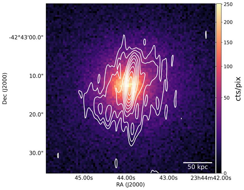
R. Timmerman et al.: VLA observations of the mini-halo and AGN feedback in the Phoenix cluster

Fig. 7. Left: spectral index map from L- and S -band images. Right: corresponding uncertainties of the spectral index map. The contours show the
L-band image smoothed to a resolution of five arcseconds and are drawn at [−1, 1, 2, 4, 8, ...] × 4σrms , where σrms = 17.9 µJy beam−1 . The circular
beam of five arcseconds is shown in the bottom-left corner.

Fig. 8. Left: spectral index map from L- and X-band images. Right: corresponding uncertainties of the spectral index map. The contours show
the X-band image smoothed to the L-band resolution and they are drawn at [−1, 1, 2, 4, 8, ...] × 4σrms , where σrms = 2.6 µJy beam−1 . The beam is
shown in the bottom-left corner.

1024 W Hz−1 . Our estimate for the size of the mini halo is smaller             We mapped the spectral index of the mini halo and derive
than that of Van Weeren et al. (2014), who estimated a size                 an integrated spectral index between the L and S bands of
in the range of 400–500 kpc using 610 MHz GMRT observa-                     −0.95 ± 0.10, which is consistent with the spectral index of
tions. This may be an indication of spectral steepening in the              −0.98 ± 0.16 as derived by Raja et al. (2020) between 610 MHz
outer regions of the mini halo, as a detection by the GMRT at               and 1.5 GHz. We were unable to find evidence for a radial gra-
610 MHz and a non-detection by the VLA at 1.5 GHz in this                   dient in the spectral index map due to the low signal-to-noise
region implies a spectral index steeper than α = −1.5, based                ratio.
on the rms noise levels in both maps. However, we do not see                    Further insight into the origin of the diffuse emission can
a trend in our spectral index maps to suggest such a spectral               be provided by the spatial correlation between the radio (IR )
steepening. In addition, the GMRT data suffers from a rela-                 and X-ray (IX ) surface brightnesses. This correlation is expected
tively poor angular resolution and sensitivity compared to the              because the relativistic electron population, and hence the radio
VLA, so we cannot make any definite claims on the spectrum                  emission, are predicted to be linked to the thermal plasma in
of the mini halo in the outer regions. Our reported value for               both hadronic and re-acceleration models. The IR –IX correla-
the radio luminosity at 1.4 GHz is consistent with previous esti-           tion allows us to constrain the distribution of the nonthermal
mates by Van Weeren et al. (2014) and Raja et al. (2020), who               ICM components with respect to the thermal plasma and thereby
calculated values of P1.4 GHz = (10.4 ± 3.5) × 1024 W Hz−1 and              investigate the origin of the radio emission (e.g., Brunetti &
P1.4 GHz = (14.38 ± 1.80) × 1024 W Hz−1 , respectively.                     Jones 2014; Ignesti et al. 2020).

                                                                                                                                  A38, page 7 of 12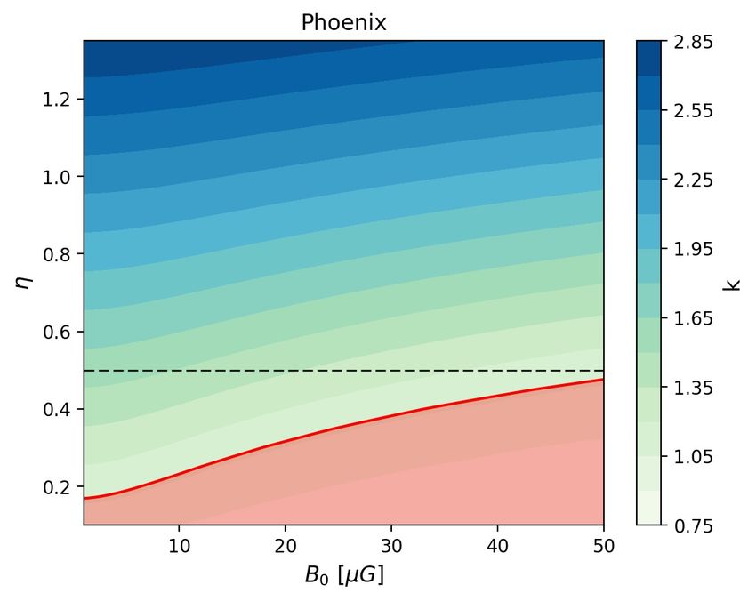
A&A 646, A38 (2021)

Fig. 9. Results from Monte Carlo point-to-point analysis. Left: an example of an estimate for k using a particular choice for the grid position. The
data points and error bars show the estimated radio surface brightness vs. X-ray surface brightness for a given grid cell. The slope of the best-fit
power law through these data (blue line) is shown in the legend. The contours in the top-left corner indicate the [3,6,12,24,48] ×σ contours of
the circularly-smoothed L-band image with a Briggs robust parameter of −1, where σ = 18 µJy. The beam size is 2.8 arcseconds circular, and is
indicated by the solid black circle. Right: histogram of all values of k from the Monte Carlo point-to-point analysis. The resulting best estimate for
kMC is reported in the legend.

     We used the Monte Carlo point-to-point analysis presented              We assume a magnetic field profile of the form
in Ignesti et al. (2020) to evaluate the IR –IX correlation for                            !η
the Phoenix cluster. We use a circularly smoothed image of                            n(r)
                                                                            B(r) = B0         ,                                                   (2)
the Phoenix cluster in the L band with a Briggs robust param-                          n0
eter of −1 to improve the resolution of the map, and thereby
reduce the area affected by AGN-related emission while simul-               where B0 and n0 are the central values of the magnetic field
taneously increasing the amount of samples of mini-halo emis-               strength and the thermal ICM number density, respectively, and
sion. The X-ray surface brightness is obtained from archival                the index η determines the scaling relation between the mag-
Chandra observations. The surface brightnesses IR and IX have               netic field and the ICM density. The constraints we derive on
been sampled with 1000 randomly-generated meshes. For the                   the magnetic field configuration are shown in Fig. 10. We find
cells in the mini-halo region, values of IR and IX are measured             that for typical values of the central magnetic field strength
and fit with a power-law relation, IR ∝ IXk , using the BCES                (10–20 µG; Carilli & Taylor 2002), we require the index η to be
algorithm (Akritas & Bershady 1996). We present in Fig. 9                   0.2–0.3, indicating that the ICM density is much more peaked
both the result of the analysis performed on a single grid (left            than the magnetic field strength. Similarly, for a typical value of
panel) and the final result of the MC routine (right panel). We             η = 0.5, we require the central magnetic field strength to be at
measured a sub-linear scaling index, k, of 0.84 ± 0.23, which               least 50 µG, which is far higher than commonly observed.
indicates that the radio emission likely declines slower than the                To provide context to these estimates of the magnetic field
X-ray emission. This result is interestingly more similar to what           configuration from the point-to-point analysis, we also calculate
is observed for giant radio halos – which often feature sub-                the equipartition magnetic field. Under the assumption that the
linear indices k in the range of 0.5 to 1.0 (Govoni et al. 2001;            magnetic field and the cosmic ray particles evolve over simi-
Feretti et al. 2001; Giacintucci et al. 2005; Hoang et al. 2019; Xie        lar timescales, they are expected to be coupled. This coupling
et al. 2020) – than to mini halos, which generally feature a super-         is supposed to lead to an equilibrium between the energy densi-
linear scaling with indices k in the range of 1.1 to 1.3 (Ignesti           ties of the cosmic ray particles and the magnetic field (Govoni
et al. 2020). Such a flat index, k, indicates that the X-ray emis-          & Feretti 2004; Beck & Krause 2005). For the classical equipar-
sion is more peaked than the radio emission, which is in agree-             tition magnetic field, we obtain a field strength of 3.4 µGauss.
ment with the exceptionally luminous cool core of this cluster.             For the revised equipartition magnetic field, we obtain a field
Therefore, it suggests that the distribution of nonthermal com-             strength of 5.5 µGauss using a commonly adopted value of
ponents does not strongly depend on the properties of the cool              γmin = 100 for the low-energy cut-off of the cosmic ray particle
core.                                                                       energy distribution. This shows that the equipartition magnetic
     On the basis of these results, we can explore the scenario of          field strength is much lower than the magnetic field strength pre-
purely hadronic origin of relativistic electrons. We followed the           dicted by a hadronic model.
approach presented in Ignesti et al. (2020) to infer the ICM mag-                In addition, we can test predictions from hadronic models
netic field to constrain the physical boundaries of the hadronic            on the spectral index of the mini-halo. According to a hadronic
model for the Phoenix cluster. We used the thermodynamic pro-               model, the radio-emitting electrons are injected by collisions
files from McDonald et al. (2015) to compute the ICM electron               between cosmic-ray protons from the AGN and thermal pro-
density and temperature. From these, we numerically calculated              tons in the ICM. This implies that the synchrotron spectral index
the X-ray emissivity. Assuming a hadronic model, we can com-                α is directly proportional to the cosmic ray proton injection
pare these to the radio emissivity expected in a pure hadronic              spectral index δ as α ≈ δ/2 (e.g., Blasi & Colafrancesco 1999;
model (e.g., Brunetti et al. 2012) to constrain the magnetic field          Pfrommer & Enßlin 2004; Brunetti et al. 2017). Therefore, our
configurations that are consistent with our value of the index k.           spectral index of α = −0.95 ± 0.10 requires a cosmic ray proton
A38, page 8 of 12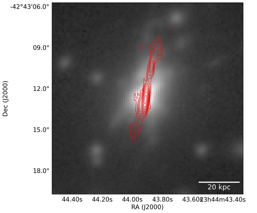
R. Timmerman et al.: VLA observations of the mini-halo and AGN feedback in the Phoenix cluster

Fig. 10. Index k for combinations of magnetic field strength and the
index η. The horizontal dashed line at η = 0.5 indicates the equilibrium
                                                                             Fig. 12. ICM cooling rate Ṁcool vs. cavity power Pcav for the sample
configuration between thermal and nonthermal energy density. The red
                                                                             of clusters from Rafferty et al. (2006). The red data point indicates
region indicates the parameter space consistent with values of k that we
                                                                             the Phoenix cluster. The gray dashed line indicates the best power-law
obtained using the Monte Carlo point-to-point analysis.
                                                                             fit through the data and is given by log Pcav [1042 erg s−1 ] = (1.00 ±
                                                                             0.10) log Ṁcool [M /yr] + (0.45 ± 0.24). All black data points are from
                                                                             Rafferty et al. (2006) and McDonald et al. (2018), and the Phoenix clus-
                                                                             ter data are from McDonald et al. (2015, 2019).

                                                                             spectral index of the mini halo are inconsistent with the values
                                                                             generally reported in literature, we conclude that our results dis-
                                                                             favor a pure hadronic origin of the radio emission, although we
                                                                             cannot exclude that proton-proton collisions played a role in the
                                                                             origin of seed electrons for the re-acceleration. Therefore, a tur-
                                                                             bulent re-acceleration model is the preferred model to explain
                                                                             the origin of the mini halo in the Phoenix cluster. However, the
                                                                             question remains as to what causes this turbulence.
                                                                                 Mazzotta & Giacintucci (2008) observed a correlation
                                                                             between the mini-halo emission and the spiral-shaped cold
                                                                             fronts produced by sloshing of the gas in the cool core
                                                                             (Markevitch et al. 2003; Ascasibar & Markevitch 2006).
                                                                             Magneto-hydrodynamic simulations by ZuHone et al. (2011a,b,
                                                                             2013, 2015) show that this sloshing can induce turbulence and
                                                                             amplify the magnetic fields required to re-accelerate thermal
                                                                             electrons to relativistic speeds. In addition, their simulations
Fig. 11. Cooling flow power versus mini-halo radio luminosity at             predict luminosities and spectral indices that are in agreement
1.4 GHz for the sample of mini halos from Giacintucci et al. (2019).         with observations. Recent research by Richard-Laferrière et al.
The red data point indicates the Phoenix cluster. The dashed grey            (2020) suggests that in addition to sloshing, AGN feedback may
line indicates the best power-law fit through the data and is given by
log PMH [1040 erg s−1 ] = (1.37±0.17) log Pcf [1040 erg s−1 ]−(6.07±0.79).
                                                                             also contribute significantly to the amount of turbulence. For the
The integrated mini-halo luminosities are from Giacintucci et al. (2019)     Phoenix cluster, we find that the extent of the mini halo matches
and this work. Values of the cooling rates and ICM temperatures are          with the extent of the sloshing pattern in the ICM observed using
from Arnaud et al. (1987), Churazov et al. (2003), Gitti & Schindler         X-ray data (see Fig. 5). Toward the south of the AGN, the mini
(2004), Böhringer et al. (2005), Covone et al. (2006), Leccardi &            halo appears to be confined to the overdense region in the ICM,
Molendi (2008), Bravi et al. (2015), McDonald et al. (2015, 2018),           whereas toward the west it appears to be confined to the under-
Main et al. (2016), and Werner et al. (2016).                                dense region in the ICM.
                                                                                 On the other hand, Gitti et al. (2002, 2004, 2007) suggested
                                                                             that the turbulence in the core can be induced by the strong cool-
injection spectral index of δ = −1.90±0.20, but such a flat distri-          ing flow accreting onto the cool core. If so, a direct relation is
bution is only marginally consistent with the generally observed             expected between the mini-halo cooling flow power Pcf and the
values of δ in the range of −2.1 to −2.4 (e.g., Völk et al. 1996;            integrated mini-halo radio power νPMH . The cooling flow power
Blasi & Colafrancesco 1999; Schlickeiser 2002; Enßlin 2003;                  is calculated as Pcf = ṀkT/µmH , where Ṁ is the mass accre-
Pinzke & Pfrommer 2010).                                                     tion rate, k is Boltzmann’s constant, T is the temperature of the
    As we find that both the magnetic field configurations                   ICM, µ is the mean molecular weight, and mH is the mass of
obtained by assuming a hadronic model and the relatively flat                a hydrogen atom. We plotted the correlation between these two
                                                                                                                                  A38, page 9 of 12
A&A 646, A38 (2021)
properties based on the Giacintucci et al. (2019) sample of mini cooling time. We plotted the cavity power versus the ICM cool-
halos, as shown in Fig. 11. As previously verified by Doria et al. ing rate for the Phoenix cluster and the sample of clusters from
(2012) and Bravi et al. (2015) using different samples, this cor- Rafferty et al. (2006), as shown in Fig. 12. Here we find that the
relation between the cooling flow power and the integrated radio Phoenix cluster is the most extreme cluster in the sample, both
power of the mini halo is indeed present. However, the rela- in terms of the cooling flow rate and the cavity power. However,
tively large intrinsic scatter suggests that this correlation may not the Phoenix cluster is consistent with the observed correlation.
indicate a causal connection between the cooling flow rate and Similarly, we plotted the radio luminosity of the jetted outflows
turbulence in the cool core. Instead, this correlation could, for at 1.4 GHz, as well as the bolometric radio luminosity, against
example, emerge due to dependence on a third parameter. the cavity power, for a sample of clusters, as shown in Fig. 13.
Therefore, we conclude that the turbulent re-acceleration This is where the Phoenix cluster does appear to be an outlier, as
model powered by sloshing is the prime candidate to explain the the cavity power is too high for both the bolometric radio lumi-
origin of the mini halo. Based on the close similarities between nosity of the lobes and their radio luminosity at 1.4 GHz. This is
the mini-halo emission region and the sloshing region, and the amplified if we plot the cooling flow rate against the bolometric
agreement between the observed spectral index and theoretical radio luminosity of the lobes, as shown in Fig. 14. In this com-
predictions, we find sloshing to be the main source of turbulence parison, the Phoenix cluster is a strong outlier in the correlation.
in the ICM, although we do not exclude that the exceptionally For its cooling flow rate, the radio lobes in the Phoenix cluster
strong cooling flow in the Phoenix cluster may have partly con- are far too faint.
tributed to the turbulence. We observe a disconnection between the radio- and the X-ray
properties of the Phoenix cluster. In the radio regime, the AGN in
the Phoenix cluster appears to be relatively modest, whereas in
5.2. The extreme feedback in the Phoenix cluster
the X-ray regime, both the AGN and the cooling flow are among
Two of the main open questions about the feedback process in the strongest of all known clusters. We suspect that this differ-
the Phoenix cluster remain: why does this cluster feature such ence between the radio and the X-ray may be caused by strong
a strong cooling flow and why are the radio and X-ray observa- time variability of the AGN on Myr timescales. In our radio
tions so disconnected. According to the explanation recently pro- observations, both the northern and southern lobes appear to be
posed by McDonald et al. (2018), the strong cooling flow could detached from the AGN, and this feature is also visible in the
be a consequence of the way the most massive clusters (such ATCA observations presented by Akahori et al. (2020). In addi-
as the Phoenix cluster) are formed. As lighter clusters merge tion, we find that the central AGN is not a perfect point source,
and form more massive clusters, their low-entropy gas content but it is elongated toward the northwest and southeast, indicating
merge relatively quickly compared to their central galaxies. This that new outflows are being detected. Outburst power has been
delayed merging of the central galaxies leads to the most mas- observed to vary from factors of several in Hydra A (Wise et al.
sive clusters having relatively underweight supermassive black 2007) to two orders of magnitude in MS0735 (Vantyghem et al.
holes powering their AGNs, as they generally have a rich and 2014) over timescales of tens of Myr. This observed variability
recent merging history. For supermassive black holes, it has been has been corroborated by numerical simulations (e.g., Li et al.
observed that the mechanical power levels off as the accretion 2015; Prasad et al. 2015), providing an explanation for the lobe
rate reaches a few percent of the Eddington rate (Russell et al. structure in the Phoenix cluster. It is possible that the sloshing in
2013). This is in contrast to the radiative power of the AGN, the ICM contributes in part to this AGN variability by displac-
which continues to increase with the accretion rate. In the con- ing the accretion material of the AGN, similar to as observed in
text of a galaxy cluster, this means that if the central supermas- A2495 by Pasini et al. (2019). However, whereas the BCG in
sive black hole is underweight, the same accretion rate of the A2495 appears to be oscillating back and forth through the cool
AGN is more likely to reach this saturation point and result in core, the BCG in the Phoenix cluster is stationary at the center
the AGN being unable to compensate for the cooling flow with of the cool core. This means that sloshing can only affect the
mechanical feedback. Verifying this explanation would require AGN activity if it inhibits the cooling flow. Detailed simulations
precise measurements of the black hole masses, which we can- by Zuhone et al. (2010) suggest that sloshing mainly introduces
not derive from our radio observations. Therefore, definitively variability in the cooling flow on timescales of 1 Gyr or more.
answering this open question is not the goal of this work. How- These timescales are too long to explain the AGN variability in
ever, we can investigate if our observations are consistent with the Phoenix cluster, so we consider it to be unlikely that sloshing
this explanation. plays a major role. In this scenario, the lack of radio luminosity
According to this explanation, the overall feedback process would be caused by a break in the AGN activity, as the only con-
in the Phoenix cluster is not abnormal. Instead, the Phoenix clus- tribution to the lobe radio luminosity is caused by a relatively
ter should simply be in the tail of the distribution. To see in which short and old outburst. This break in the AGN activity would
aspects the Phoenix cluster is an outlier to the general popula- not necessarily affect the currently observed cavity power, as
tion, we looked into its cavity power and ICM cooling rate. The the cavities require time to expand, and they are therefore more
cavity power Pcav of a cluster can be estimated by dividing the dependent on a later stage of an outburst. However, the current
total enthalpy Ecav of the cavities by the buoyant rise time. Here, volume of the cavities will not be sustainable due to this AGN
the total enthalpy Ecav can be calculated as Ecav = 4 PV, where variability. As the break in the outflows reaches the cavities, they
P is the total pressure of the ICM at the position of the cavities will deflate, resulting in the average cavity power likely being
and V is the volume of the cavities. The buoyant rise time is the lower than the presently observed value.
time required for the cavities to move from the AGN to their Finally, the relatively low amount of jet precession observed
present position under the assumption that they rise through the in the Phoenix cluster by Akahori et al. (2020) and our
ICM buoyantly. The ICM cooling rate within a particular radius X-band observations likely also contributes to the low ICM re-
indicates how much mass in the ICM cools down per year due to heating efficiency of the mechanical feedback, as the energy
the emission of thermal bremsstrahlung, and it can be calculated from the AGN is not distributed isotropically, but rather pre-
as the ICM mass enclosed within the given radius divided by the dominantly in the direction of the jets. The explanation by
A38, page 10 of 12R. Timmerman et al.: VLA observations of the mini-halo and AGN feedback in the Phoenix cluster
Fig. 13. Left: radio luminosity of the lobes at 1.4 GHz vs. cavity power for Phoenix cluster (red) and the Bîrzan et al. (2008) sample of mini halos
(black). The dashed line shows the best power-law fit through the data and is given by log Pcav [1042 erg s−1 ] = (0.86±0.20) log P1400 [1024 W Hz−1 ]+
(1.63 ± 0.29). Right: bolometric radio luminosities of the lobes between 10 MHz and 10 GHz for the same sample. The dashed line shows the best
power-law fit through the data and is given by log Pcav [1042 erg s−1 ] = (0.79 ± 0.15) log Lradio [1042 erg s−1 ] + (2.03 ± 0.19). Phoenix cluster data are
from McDonald et al. (2019) and this work, and data for the other clusters are from Bîrzan et al. (2008).
McDonald et al. (2018) combined with time variability of the
AGN activity and a low jet precession angle may resolve some
of the remaining open questions on the AGN feedback in
the Phoenix cluster, although a more quantitative investigation
would be required to confirm the validity of this model.
6. Conclusions
In this paper, we present new Karl G. Jansky Very Large Array
observations, enabling the radio lobes of the AGN and the mini
halo in the Phoenix cluster to be studied in detail at frequen-
cies from 1 to 12 GHz. In particular, our observations resolve
the radio lobes of the AGN in all four frequency bands, and the
mini halo can be detected in both our L and S bands. Using these
multifrequency observations, we studied the remarkable feed-
back scenario in the Phoenix cluster and the origin of its mini
halo.
We find that the total flux density of the source at 1.5 GHz is
33.8 ± 1.7 mJy, with an overall spectral index of −1.12 ± 0.02.
Using our L- and S -band observations, we find that the mini
halo has an average spectral index of −0.95 ± 0.10. By sub- Fig. 14. ICM cooling rate Ṁcool vs. bolometric radio luminosity of lobes
tracting compact emission and through radial profile fitting, between 10 MHz and 10 GHz. The red data point indicates the Phoenix
we find that the mini halo has a total flux density at 1.5 GHz cluster, and the black data points indicate the sample of Bîrzan et al.
of 8.5 ± 0.9 mJy, which corresponds to a radio luminosity at (2008). The dashed line shows the best power-law fit through the data
1.4 GHz of (13.0 ± 1.4) × 1024 W Hz−1 . In addition, we find and is given by log Lradio [1042 erg s−1 ] = (1.41±0.35) log Ṁcool [M /yr]−
that the mini halo has a maximum observable radius in the (1.95 ± 0.53). Phoenix cluster data are from McDonald et al. (2019) and
this work, and data for the other clusters are from Bîrzan et al. (2008),
L band of 240 kpc. At 1.5 GHz, the radio lobes show a total
McDonald et al. (2019).
flux density of 7.6 ± 0.8 mJy, and spectral indices with respect
to 10 GHz of −1.35 ± 0.07 (northern lobe) and −1.30 ± 0.12
(southern lobe).
Due to the relatively flat spectral index of the mini halo, cies, and we find our integrated spectral index of the mini halo
the low index k, and the extreme magnetic field configuration to be consistent with numerical predictions for a turbulent re-
we obtain by assuming a hadronic model, we conclude that our acceleration model. For these reasons, we conclude that a turbu-
results disfavor a pure hadronic origin of the mini halo. On the lent re-acceleration model is the preferred model to explain the
contrary, we confirm the correlation between the cooling flow origin of the mini halo, and in particular we favor sloshing in the
power and the radio luminosity of the mini halo with respect cool-core as an explanation for the turbulence.
to other clusters. Also, we observe the sloshing pattern in the By measuring the flux density of the radio lobes in the L
ICM to match with the extent of the mini halo at radio frequen- band for the first time, the mechanical feedback in the Phoenix
A38, page 11 of 12A&A 646, A38 (2021)
cluster has been studied from a radio perspective. We observe Gitti, M., Ferrari, C., Domainko, W., et al. 2007, A&A, 470, L25
a disconnection between the X-ray and radio properties of the Gitti, M., Brighenti, F., & McNamara, B. R. 2012, Adv. Astron., 2012, 950641
Phoenix cluster: the cavity power and cooling flow rate are both Govoni, F., & Feretti, L. 2004, Int. J. Mod. Phys. D, 13, 1549
Govoni, F., Enßlin, T. A., Feretti, L., & Giovannini, G. 2001, A&A, 369, 441
among the most extreme ever measured, whereas the bolomet- Gull, S. F., & Northover, K. J. E. 1973, Nature, 244, 80
ric radio luminosity of the lobes is relatively modest. We find Hlavacek-Larrondo, J., McDonald, M., Benson, B. A., et al. 2014, ApJ, 805, 35
that the feedback in the Phoenix cluster is overall consistent Hoang, D. N., Shimwell, T. W., van Weeren, R. J., et al. 2019, A&A, 622, A20
with the proposed explanation by McDonald et al. (2018), which Ignesti, A., Brunetti, G., Gitti, M., & Giacintucci, S. 2020, A&A, 640, A37
states that the strong cooling rate and inefficient feedback are Kitayama, T., Ueda, S., Akahori, T., et al. 2020, PASJ, 72, 33
characteristic of more massive clusters. Strong time variability Lagos, C. D. P., Cora, S. A., & Padilla, N. D. 2008, MNRAS, 388, 587
Leccardi, A., & Molendi, S. 2008, A&A, 486, 359
of the AGN activity on Myr timescales may explain the dis- Li, Y., Bryan, G. L., Ruszkowski, M., et al. 2015, ApJ, 811, 73
connection between the radio and the X-ray properties of the Main, R. A., McNamara, B. R., Nulsen, P. E. J., et al. 2016, MNRAS, 464, 4360
system. Finally, a small amount of jet precession likely also Markevitch, M., & Vikhlinin, A. 2007, Phys. Rep., 443, 1
contributes to the low ICM re-heating efficiency of the AGN Markevitch, M., Vikhlinin, A., & Forman, W. R. 2003, in Matter and Energy in
Clusters of Galaxies, ASP Conf. Ser., 301, 37
feedback. Mathews, W. G., & Guo, F. 2011, ApJ, 738, 155
For future research, it would be valuable to obtain more Matteo, T. D., Springel, V., & Hernquist, L. 2005, Nature, 433, 7026
high-resolution radio observations of a sample of mini halos Mauch, T., Murphy, T., Buttery, H. J., et al. 2003, MNRAS, 342, 1117
to further test the correlation between the mini-halo emission Mazzotta, P., & Giacintucci, S. 2008, ApJ, 675, L9
and the sloshing pattern in the ICM, as this could provide McDonald, M., Baybliss, M., Benson, B. A., et al. 2012, Nature, 488, 349
McDonald, M., Benson, B., Veilleux, S., et al. 2013, ApJ, 765, L37
very strong evidence for the turbulent re-acceleration model, McDonald, M., Swinbank, M., Edge, A. C., et al. 2014, ApJ, 784, 18
and current results look promising. In addition, low-frequency McDonald, M., McNamara, B. R., van Weeren, R. J., et al. 2015, ApJ, 811, 111
observations may test whether the sloshing of the ICM pro- McDonald, M., Gaspari, M., McNamara, B. R., & Tremblay, G. R. 2018, ApJ,
duces more extended, ultra-steep spectrum emission beyond the 858, 45
cold fronts, as observed in the cases of PSZ1G139.61+24 and McDonald, M., McNamara, B. R., Voit, G. M., et al. 2019, ApJ, 885, 63
McMullin, J. P., Waters, B., Schiebel, D., Young, W., & Golap, G. 2007, in CASA
RXJ1720.1+2638 by Savini et al. (2018, 2019). Architecture and Applications, 376, 127
McNamara, B. R., & O’Connell, R. W. 1989, AJ, 98, 2018
Acknowledgements. We would like to thank the anonymous referee for useful McNamara, B. R., & Nulsen, P. E. J. 2007, ARA&A, 45, 117
comments. RT and RJvW acknowledge support from the ERC Starting Grant McNamara, B. R., & Nulsen, P. E. J. 2012, New J. Phys., 14, 055023
ClusterWeb 804208. Support for this work was provided to MM by NASA Menci, N., Fontana, A., Giallongo, E., et al. 2006, ApJ, 647, 753
through Chandra Award Number GO7-18124 issued by the Chandra X-ray Offringa, A. R., de Bruyn, A. G., Biehl, M., et al. 2010, MNRAS, 405, 155
Observatory Center, which is operated by the Smithsonian Astrophysical Obser- Offringa, A. R., McKinley, B., & Hurley-Walker, N., et al. 2014, MNRAS, 444,
vatory for and on behalf of the National Aeronautics Space Administration under 606
contract NAS8-03060. Page, M. J., Symeonidis, M., Vieira, J. D., et al. 2012, Nature, 485, 213
Pasini, T., Gitti, M., Brighenti, F., et al. 2019, ApJ, 885, 111
Perley, R. A., & Butler, B. J. 2013, ApJS, 204, 19
References Perley, R. A., & Butler, B. J. 2017, ApJS, 230, 7
Pfrommer, C., & Enßlin, T. A. 2004, A&A, 413, 17
Akahori, T., Kitayama, T., Ueda, S., et al. 2020, PASJ, 72, 62 Pinzke, A., & Pfrommer, C. 2010, MNRAS, 409, 449
Akritas, M. G., & Bershady, M. A. 1996, ApJ, 470, 706 Prasad, D., Sharma, P., & Babul, A. 2015, ApJ, 811, 108
Arnaud, K. A., Johnstone, R. M., Fabian, A. C., et al. 1987, MNRAS, 227, Rafferty, D. A., McNamara, B. R., Nulsen, P. E. J., & Wise, M. W. 2006, ApJ,
241 652, 216
Ascasibar, Y., & Markevitch, M. 2006, ApJ, 650, 102 Raja, R., Rahaman, M., Datta, A., et al. 2020, ApJ, 889, 128
Beck, R., & Krause, M. 2005, Astron. Nachr., 326, 414 Rasia, E., Borgani, S., Murante, G., et al. 2015, ApJ, 813, L17
Böhringer, H., Burwitz, V., Zhang, Y. Y., et al. 2005, ApJ, 633, 148 Richard-Laferrière, A., Hlavacek-Larrondo, J., Nemmen, R. S., et al. 2020,
Bîrzan, L., McNamara, B. R., Nulsen, P. E. J., et al. 2008, ApJ, 686, 859 MNRAS, 499, 2934
Blasi, P., & Colafrancesco, S. 1999, Astropart. Phys., 12, 169 Russell, H. R., McNamara, B. R., Edge, A. C., et al. 2013, MNRAS, 432, 530
Bonafede, A., Intema, H. T., Brüggen, M., et al. 2014, MNRAS, 444, L44 Russell, H. R., McDonald, M., McNamara, B. R., et al. 2017, ApJ, 836, 130
Bravi, L., Gitti, M., & Brunetti, G. 2015, MNRAS, 455, L41 Savini, F., Bonafede, A., Brüggen, M., et al. 2018, MNRAS, 478, 2234
Briggs, D. S. 1995, PhD Thesis, New Mexico Institude of Mining and Savini, F., Bonafede, A., Brüggen, M., et al. 2019, A&A, 622, A24
Technology Schlickeiser, R. 2002, Cosmic Ray Astrophysics (Springer)
Brüggen, M., & Kaiser, C. R. 2002, Nature, 418, 301 Sijacki, D., Springel, V., Matteo, T. D., & Hernquist, L. 2007, MNRAS, 380, 877
Brunetti, G., & Jones, T. W. 2014, Int. J. Mod. Phys. D, 23, 1430007 Ueda, S., Hayashida, K., Anabuki, N., et al. 2013, ApJ, 778, 33
Brunetti, G., Blasi, P., Reimer, O., et al. 2012, MNRAS, 426, 956 Vantyghem, A. N., McNamara, B. R., & Russell, H. R. 2014, MNRAS, 442,
Brunetti, G., Zimmer, S., & Zandanel, F. 2017, MNRAS, 472, 1506 3192
Carilli, C. L., & Taylor, G. B. 2002, ARA&A, 40, 319 Van Weeren, R. J., Intema, H. T., Lal, D. V., et al. 2014, ApJ, 786, L17
Churazov, E., Forman, W., Jones, C., & Böhringer, H. 2003, ApJ, 590, 225 Van Weeren, R. J., de Gasperin, F., Akamatsu, H., et al. 2019, Space Sci. Rev.,
Ciotti, L., Ostriker, J. P., & Proga, D. 2010, ApJ, 717, 708 215, 16
Covone, G., Adami, C., Durret, F., et al. 2006, A&A, 460, 381 Vogelsberger, M., Genel, S., Springel, V., et al. 2014, Nature, 509, 177
Croton, D. J., Springel, V., White, S. D. M., et al. 2006, MNRAS, 365, 11 Völk, H. J., Aharonian, F. A., & Breitschwerdt, D. 1996, Space Sci. Rev., 75,
Doria, A., Gitti, M., Ettori, S., et al. 2012, ApJ, 753, 47 297
Enßlin, T. A. 2003, A&A, 399, 409 Werner, N., Zhuravleva, I., Canning, R. E. A., et al. 2016, MNRAS, 460, 2752
Fabian, A. C. 1994, ARA&A, 32, 277 Williamson, R., Benson, B. A., High, F. W., et al. 2011, ApJ, 738, 139
Fabian, A. C. 2012, ARA&A, 50, 455 Wise, M. W., McNamara, B. R., & Nulsen, P. E. J. 2007, ApJ, 659, 1153
Fabian, A. C., Nulsen, P. E. J., & Cranizares, C. R. 1982, MNRAS, 201, 933 Xie, C., van Weeren, R. J., Lovisari, L., et al. 2020, A&A, 636, A3
Feretti, L., Fusco-Femiano, R., Giovannini, G., & Govoni, F. 2001, A&A, 373, Zuhone, J. A., Markevitch, M., & Johnson, R. E. 2010, ApJ, 717, 908
106 ZuHone, J. A., Markevitch, M., & Brunetti, G. 2011a, Mem. Soc. Astron. It., 82,
Fujita, Y., Kohri, K., Yamazaki, R., & Kino, M. 2007, ApJ, 663, L61 632
Giacintucci, S., Venturi, T., Brunetti, G., et al. 2005, A&A, 440, 867 ZuHone, J. A., Markevitch, M., & Lee, D. 2011b, ApJ, 743, 16
Giacintucci, S., Markevitch, M., Cassano, R., et al. 2019, ApJ, 880, 70 ZuHone, J. A., Markevitch, M., Brunetti, G., & Giacintucci, S. 2013, ApJ, 762,
Gitti, M., & Schindler, S. 2004, A&A, 427, L9 78
Gitti, M., Brunetti, G., & Setti, G. 2002, A&A, 386, 456 ZuHone, J. A., Brunetti, G., Giacintucci, S., & Markevitch, M. 2015, ApJ, 801,
Gitti, M., Brunetti, G., Feretti, L., & Setti, G. 2004, A&A, 417, 1 146
A38, page 12 of 12You can also read