Hyperspectral Imaging for Color Adulteration Detection in Red Chili - MDPI
←
→
Page content transcription
If your browser does not render page correctly, please read the page content below
applied
           sciences
Article
Hyperspectral Imaging for Color Adulteration
Detection in Red Chili
Muhammad Hussain Khan 1 , Zainab Saleem 1 , Muhammad Ahmad 1, *                  , Ahmed Sohaib 1 ,
Hamail Ayaz 1 and Manuel Mazzara 2
 1    Advance Image Processing Research Lab (AIPRL), Department of Computer Engineering,
      Khwaja Fareed University of Engineering and Information Technology, Rahim Yar Khan 64200, Pakistan;
      hussain.khan@kfueit.edu.pk (M.H.K.); zainab.saleem@kfueit.edu.pk (Z.S.);
      ahmed.sohaib@kfueit.edu.pk (A.S.); hamail.ayaz@kfueit.edu.pk (H.A.)
 2    Institute of Software Development and Engineering, Innopolis University, 420500 Innopolis, Russia;
      m.mazzara@innopolis.ru
 *    Correspondence: mahmad00@gmail.com

 Received: 6 July 2020; Accepted: 18 August 2020; Published: 28 August 2020

 Abstract: The quality of red chili is characterized based on its color and pungency. Several factors
 like humidity, temperature, light, and storage conditions affect the characteristic qualities of red chili,
 thus preservation required several measures. Instead of ensuring these measures, traders are using
 oil and Sudan dye in red chili to increase the value of an inferior product. Thus, this work presents
 the feasibility of utilizing a hyperspectral camera for the detection of oil and Sudan dye in red chili.
 This study describes the important wavelengths (500–700 nm) where different adulteration affects
 the response of the reflected spectrum. These wavelengths are then utilized for training an Support
 Vector Machine (SVM) algorithm to detect pure, oil-adulterated, and Sudan dye-adulterated red
 chili. The classification performance achieves 97% with the reduced dimensionality and 100% with
 complete validation data. The trained algorithm is further tested on separate data with different
 adulteration levels in comparison to the training data. Results show that the algorithm successfully
 classifies pure, oil-adulterated, and Sudan-adulterated red chili with an accuracy of 100%.

 Keywords: hyperspectral imaging; red chili; edible oil; sudan dye; PCA; SVM

1. Introduction
      Red chili is a spice, fruit, and vegetable consumed across the globe from ancient times as fresh,
dried, crushed, or in powdered form. It has also been widely used in different sauces and medicines.
The quality of red chili is characterized based on its color and pungency. Capsaicinoids are the
main component in red chili, which cause a sensation of burning when they come in to contact
with body tissues and the level of burning sensation is measured in Scoville Heat Units (SHU).
The color of red chili is due to the presence of carotenoids, which come in different isomeric forms and
derivatives. This makes it difficult to measure the color of red chili. However, the American Spice and
Trade Association (ASTA) has devised a mechanism for measuring red chili color by calculating the
absorbance at 460 nm [1].
      In a natural environment, carotenoids in red chili are well protected but storage conditions highly
impact the carotenoid content. Schweigert et al. reported that the amount of carotenoids loss varies
from 9.6% to 16.7% during storage with and without illumination, respectively [2]. Other studies
examined different factors (like temperature, humidity, and water) of storage conditions and their
impact on the color of red chili [3,4]. Similarly, the process of drying also affects the carotenoids content
in red chili. Minguez-Mosquera et al. reported that drying of red chili at mild temperature provides
the time for necessary metabolic activities which increases or retains the number of carotenoids [5].

Appl. Sci. 2020, 10, 5955; doi:10.3390/app10175955                             www.mdpi.com/journal/applsci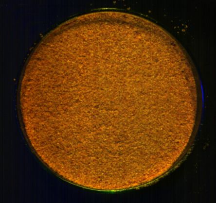
Appl. Sci. 2020, 10, 5955 2 of 17
In general, to preserve the color or carotenoids content of red chili, several measures including
closed storage, lower temperature, and humidity are required. However, instead of ensuring these
measures, traders have found another alternative of deceiving the customers. To enhance the color or
increase the value of the inferior product, Sudan dyes that are characterized as a carcinogen [6] and
banned worldwide as a food additive were found in grounded red chili and products that contain red
chilies like sauces, cuisines, and frozen meat.
Sudan dyes are insoluble in water but can be dissolved in fats and some organic solvents [7].
However, there is very little information available about their solubility in the literature. The main
reason for adding Sudan dyes in red chili instead of approved food color is its insolubility in water.
This property helps traders in hiding their fraud as food colors are soluble in water and can change the
color of the food in which color-adulterated red chili is added. Being insoluble in water, Sudan dyes
do not alter the color properties of food.
Moreover, as Sudan dyes are available in powdered form and cannot be added directly in
grounded red chili, they are usually dissolved first in oil and then mixed in grounded red chili.
Although the oil used is mostly edible, it is still harmful to someone who is allergic to the oil or facing
specific health conditions. Moreover, oil without any Sudan dye also changes the color properties of
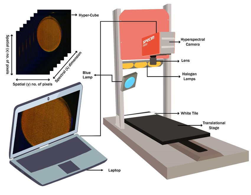
red chili as shown in Figure 1.
Pure Red Chili Oil-Adulterated Red Chili
Figure 1. Visual difference of pure and oil-adulterated red chili.
Although Sudan dyes were banned as food additives in 1973 by a joint committee of the Food and
Agriculture Organization (FAO) and World Health Organization (WHO) on food additives due to its
toxicity [8], their usage has continued in different foods like palm oil, red chili, and others. This issue
came to the surface in 2003 when a lab detected Sudan dye in red chili imported from India, and the
European Union then took emergency measures and published a list of authorized food color [9].
As a result, in 2005 the United Kingdom Food Safety Agency (FSA) analyzed over 400 products and
found some to be contaminated with Sudan dye [10]. Similar incidents were observed in India, China,
Pakistan, and South Africa, forcing countries to implement safety measures and develop detection
methods for illegal dyes in their food [11–13].
There are several traditional methods available for the detection of Sudan dyes in red chili
like Thin-Layer Liquid Chromatography (TLC) [7], High-Performance Liquid Chromatography [14],
and their modified usage like HPLC with photodiode arrays [15]. However, these methods are
laborious and require skilled workers. Moreover, they are not portable, and sending samples to distant
laboratories took considerable time and effort.
Imaging techniques have been widely used in agriculture and food industries for quality control;
inspection; and monitoring of growth, disease, etc. However, a digital camera, similar to the human
eye, is only capable of working in a visible spectrum of electromagnetic radiations. This limits the
examination to physical attributes like the color, size, and shape of the object. To determine the
chemical properties of an agro-food, spectroscopic methods are usually utilized which provide the
Appl. Sci. 2020, 10, 5955                                                                           3 of 17

mean spectrum of a sample without any spatial information [16]. Thus, these methods are limited to
homogenized samples and cannot be used for the inspection of heterogeneous objects.
      In recent years, several vibrational spectroscopic techniques like Raman, Infrared (IR),
and Ultraviolet–Visible (UV–Vis) have been utilized with chemometric analysis to detect and measure
various properties of red chili. Jongguk Lim et al. presented a system that can measure the moisture
and capsaicinoids content of red chili by using Visible and Near-Infrared (VIS–NIR) spectroscopy [17].
Smita Tripathi and H.N. Mishra proposed the use of Fourier transform near-infrared (FT-NIR)
spectroscopy for the detection of aflatoxin B1 in red chili [18]. Xi-YU Wu et al. present an approach for
the detection of adulterants in grounded Sichuan pepper powder using VIS-NIR spectroscopy [19].
Haughey et al. studied the feasibility of utilizing Near-Infrared (NIR) and Raman Spectroscopy for the
detection of Sudan dye in red chili powder [20]. They spiked red chili powder with Sudan I dye and
used Partial Least Squares Discriminate Analysis (PLS-DA) for the detection of Sudan dye. Similarly,
Di Anibal et al. utilized UV-VIS, Raman, and FT-NIR spectroscopy techniques for the detection of
Sudan dye in various spices including paprika. They mixed Sudan dye in chloroform and spiked
spices with the solution. They further used K-Nearest Neighbor (KNN), Soft Independent Modeling of
Class Analogy (SIMCA), and PLS-DA for classification. [21,22].
      Hyperspectral imaging combines the power of both tools (digital camera and spectroscopy) and
extends the capabilities to a new dimension [23]. As a traditional probe-based spectroscopy method,
it acquires the spectrum of a sample, and conventional imaging techniques map this information
in spatial dimension for visualization. Hyperspectral cameras were developed and utilized initially
for remote sensing [24], but the recent advancement in technologies has introduced this tool in
laboratories. Thus, researchers started utilizing its powers in various fields like agriculture [25],
food [26], pharmaceutical [27], forensic [28], and environment [29]. This tool has several advantages
such as being precise, expeditious, noninvasive, and multi-analytical, which enable it to predict several
attributes (physical and chemical) with a single acquisition.
      The Hyperspectral Imaging (HSI) system provides the data in the form of a 3D cube usually
known as hypercube [30]. The hypercube consists of multiple spatial images stacked concerning
wavelength spectrum. The coordinates of a hypercube are labeled as x, y, and λ, where x and y
represent the spatial coordinates, and λ is the spectral coordinate [31].
      In our previous work [32], we have utilized the (VIS-NIR) HSI system with a one-class Support
Vector Machine (SVM), to detect powder adulterants in grounded red chili. To ensure purely grounded
red-chili, we purchased whole chili samples from the market and ground it by ourselves. Our system
was up to 99% effective. However, when we extend our experimentation to locally available grounded
red chili, the results varied sharply. The system was able to recognize red chili but predicting very high
adulterant concentration. We obtained different samples from the local market but the results were
the same, while the grounded red chili of multinational companies like National Foods, Shan Foods,
Habib Food, and Mehran Foods was predicted accurately by our algorithm.
      Therefore, a proposition was made that there was something different in the process which we are
neglecting while grinding by ourselves. Initially, we visited a local company to observe their process of
grinding and found out that we were using a household mixer grinder that utilizes blades for crushing,
while in local industry stone-based grinders are used. Therefore, a stone-based grinder was acquired
and multiple chili samples were ground. We trained our model on the newly prepared samples but
the results were not different from the previous ones. Our algorithm predicted the correct proportion
of adulterants in stone grounded red chili.
      While observing the mean spectrum of samples acquired from the local market and grounded by
ourselves, we noticed a groove in the locally grind red chili from 650 to 680 nm (Figure 2). This dip
was not found in any of our grind samples, either in household mixer grinder or stone-based grinders.
In further investigation, we found out that the local industry is adding edible oil while grounding red
chili to increase the shine without knowing its a type of adulteration. Furthermore, humidity increases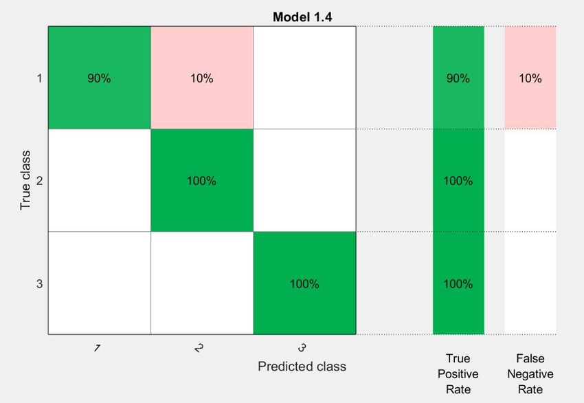
Appl. Sci. 2020, 10, 5955                                                                                                       4 of 17

in the air as the rainy season began. Red chili without proper storage facility starts losing its color
swiftly in this season. Therefore, vendors mix Sudan dyes in oil to make red chili color artificially.

                                                                              Mean Reflectance
                         1

                        0.9           Self-Processed Grouded Red Chili
                                      Locally-Acquired Grounded Red Chili
                        0.8

                        0.7
          Reflectance

                        0.6

                        0.5

                        0.4

                        0.3

                        0.2

                        0.1

                         0
                                500         550         600         650     700        750       800   850   900   950   1000
                                                                                  Wavelength

                              Figure 2. Mean reflectance spectra of locally acquired and self-grounded red chili.

      In this work, we have analyzed a new adulterant, i.e., edible oil, which is not studied before but
only reported in news [33]. We have also discussed market practices for the addition of Sudan dye in
red chili and presented a novel method for the detection of oil and Sudan dye adulterated red chili by
using an HSI system in the range of 395 to 1000 nm with multi-class SVM.
      The proposed methodology works in the following way. First, important wavelengths were
identified for oil and Sudan dye adulteration. Second, Savitzky-Golay differentiation was utilized to
remove the baseline of spectra and preserve important spectral features. Third, to make the model
robust, Principal Component Analysis (PCA) was used to remove redundant information, and finally
a multi-class SVM model is trained on pure chili, oil-adulterated chili, and Sudan dye-adulterated
chili. The trained model can differentiate pure chili from adulterated with an accuracy of 97%, which is
further increased up to 100% by eliminating PCA in our process.

2. Experimental Data Set
      In this research, two types of red chilis have been considered: Kunri and hybrid. Kunri is produced
in the Sindh province of Pakistan, while hybrid chili is imported from Rajasthan, India. The whole
chili was acquired from the local market and ground using a stone grinder. As the stone grinding
produces intense heat which can burn the color of red chili, samples were cooled several times during
the grinding process. Being low cost, mustard oil is mostly used as an adulterant to enhance the color
of red chili. However, for this study, we have considered two types of edible oils: mustard and olive.
Both types of oil with ordinary quality were procured from the local market. Each type of oil was
added in both types of red chili with 30 g for each sample. The oil quantity was increased by 1 mL to
10 mL for each sample. Twenty samples of each oil-contaminated red chili were prepared with four
samples as pure.
      For the sample preparation of Sudan dye (IV)-adulterated red chili, 1 g and 2 g of Sudan dye (IV)
were mixed in 30 mL of mustard oil separately. The samples were blended thoroughly to dissolve
Sudan dye in the oil. A similar procedure was carried out as mentioned for pure oils for mixing
Sudan mixed oil to the red chili. Therefore, a total of 80 adulterated samples and 8 pure samples
were prepared. To homogenize the samples, each sample was mixed using a household mixer grinder.
The details of prepared samples are given in Table 1.

Test Data Set
     In addition to the samples explained above, an additional data set is prepared for the testing of the
designed algorithm with different proportions of oil and Sudan dye mixed oil (1.5, 3.5, 5.5, 7.5, 8.5 mL).
The details of the prepared samples are given in Table 2.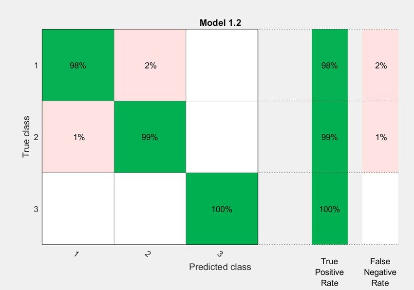
Appl. Sci. 2020, 10, 5955                                                                              5 of 17

                                Table 1. Total samples prepared for each adulterant.

                                          Sample Details                 Total Sample
                                       Pure Red Chili (Kunri)                      4
                                      Pure Red Chili (Hybrid)                      4
                                Chili Adulterated with mustard oil                20
                                  Chili Adulterated with olive oil                20
                               Chili Adulterated with sudan dye (1g)              20
                               Chili Adulterated with sudan dye (2g)              20
                                           Total Sample                           88

                                        Table 2. Test data set samples details.

                                         Sample Details                                Total Samples
                                       Pure Red Chilli (Kunri)                               4
                                      Pure Red Chilli (Hybrid)                              4
                       Chili (Kunri + Hybrid) Adulterated with mustard oil                 5+5
                          Chili (Kunri + Hybrid) Adulterated with olive oil                5+5
                     Chili (Kunri + Hybrid) Adulterated with Sudan dye (0.5 g)             5+5
                     Chili (Kunri + Hybrid) Adulterated with Sudan dye (1.5 g)             5+5
                                           Total Samples                                    48

     The data set was labeled as Pure (class “1”), Oil-adulterated (class “2”), and Sudan dye-adulterated
(class “3”).

3. Methods
      This section describes the procedure we followed to classify oil and Sudan dye-adulterated
chili from pure. The section explains the hyperspectral imaging system, the mode of acquisition,
the mathematical preprocessing applied to the acquired data before training our algorithm, and the
importance of these techniques. Moreover, data reduction using PCA and SVM is also explained in
the context of this study. For the processing of data, MATLAB 2019 software by Math Works has been
used with the image processing toolbox [34].

3.1. Hyper Spectral Imaging System
     In this study, a hyperspectral camera (FX-10, Specim, Spectral Imaging Ltd., Oulu, Finland) was
used. The camera was pre-equipped with a special lens from Scheiner (Cinegon 1.4/8 mm). As the
camera works on the principle of line scan (one thin line of the object with full spectra at a time),
it was mounted on a lab scanner to scan the complete sample. The scanner has a moving platform
of 40 × 20 cm, three halogen lamps for illumination, and a camera mounting plate. The height of
the camera mounting plate is adjustable thus it is kept 6 cm above from the sample. The height
adjustment was made after several iterations to ensure the field of view almost equal to the sample.
This adjustment enhanced the spatial resolution of the camera. The scanner was connected to a laptop
directly via serial communication port, while for the camera the GigE-Vision interface was used to
transfer data on a laptop. The complete experimental set-up is shown in Figure 3.
     In our previous work [32], we described the limitation of halogen bulb in blue wavelength.
However, for this study, we minimized this limitation by installing two further light sources: blue and
ultraviolet. The blue source covers the range of wavelength from 410 to 440 nm, while the ultraviolet
source covers a range from 395 to 410 nm. These additional light sources increase the signal to noise
ratio (as shown in Figures 4 and 5) in the starting bands of a camera and decreased noise variations in
the spectrum over the entire range of the camera, i.e., 395–1000 nm.
Appl. Sci. 2020, 10, 5955                                                                                                       6 of 17

                                                     Figure 3. Hyperspectral imaging system.

                  Halogen and Blue Light Source                                                      Halogen Light Response

                                               Figure 4. Red chili spectral response at 440 nm.

                                                                                  Mean Reflectance
                                    1
                                                Without Blue-Light Source

                                                With Blue-Light Source

                                  0.8

                                  0.6
                    Reflectance

                                  0.4

                                  0.2

                                    0

                                  -0.2
                                         400   500                          600         700           800       900      1000
                                                                                    Wavelength

                       Figure 5. Spectral signature difference with the addition of blue light source.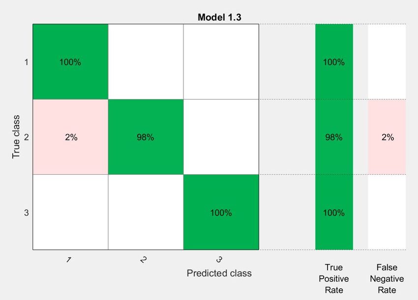
Appl. Sci. 2020, 10, 5955                                                                                                                            7 of 17

3.2. Data Acquisition
     The prepared samples were placed in a Petri dish. To avoid diffraction and shadowing,
samples were leveled using a surface leveler. The leveled samples were placed on the moving bed
of the scanner. A white tile of 99.9% reflectance value was also placed on the moving platform along
with samples for reference. The reference object was placed along with all samples for calculation
of reflectance described in Section 3.3. The platform was then put in motion at a speed of 20 m/s
while the frame rate of the camera was set at 60 Hz. The exposure was controlled manually using an
aperture of the lens and kept constant for all samples. The following procedure was followed for data
acquisition of samples.

1.    The camera’s shutter was closed and 100 dark frames were acquired. A large number of frames
      were acquired to record the sensor’s response fully. The mean noise spectra of the camera are
      shown in Figure 6.
2.    The lab scanner transnational platform was moved to the position where the white reference is
      placed and the camera captures 100 frames of the white tile. The mean spectral response of white
      tile is shown in Figure 7.
3.    The lab scanner transnational platform was moved to the sample’s position and scanned the
      sample line by line. The reflected spectrum of the chili sample is shown in Figure 7.

                                                                               Dark Reference
                                179

                               178.5

                                178
                Camera Noise

                               177.5

                                177

                               176.5

                                176
                                       400             500         600               700               800         900                        1000
                                                                               Wavelength(nm)

                       Figure 6. Hyperspectral camera internal noise captured by acquiring dark frames.

                               1600
                                                                                                                   Sample Radiance
                               1400                                                                                White Reference Radiance

                               1200

                               1000
                Radiance

                               800

                               600

                               400

                               200

                                  0
                                  300            400         500         600         700         800         900         1000                 1100
                                                                               Wavelength (nm)

                                             Figure 7. Reflected energy from the reference material and sample.

     The numbers of dark and white frames along with the position of white reference, target start,
and target stop were adjusted in Lumo Scanner Software to control the position of transnational
platform and acquisition of samples. A total of 3 files were stored in .raw format for each sample:
dark reference, white reference, and sample. Along with these files, a false-color RGB image was also
Appl. Sci. 2020, 10, 5955 8 of 17
formed using the spectral response of the object at 430 nm, 510 nm, and 670 nm to visualize the scanned
sample. The sample and reference data were loaded in MATLAB in the form of a 3D cube using a
multiband-read command. The cube consists of 224 spectral images having the radiance information
of scanned object at the spectral range of 395 to 1000 nm with the spectral full width at half maximum
of 5.5 nm.
3.3. Spectral Reflectance
The hyperspectral sensor records spectral radiance which depends on several factors including
illumination, atmospheric effects, the geometry of the object, and the sensor’s characteristics.
Controlling these factors will require a lot of effort, time, capital, and sometimes it is physically
impossible [35]. To remove these effects from the acquired radiance data spectral, reflectance needs
to be calculated. Spectral reflectance is defined as the ratio of reflected incident light energy [36].
The incident light is measured after reflection from a reference material of known reflectance. As the
reference material is placed with samples, it is safe to assume that the reflected energy from the
reference material has also experienced the same effects as the energy which is reflected from samples.
For the sensor’s characteristics response, frames were captured while keeping the shutter closed.
Therefore, these acquired frames provided information regarding the sensitivity of the camera at each
wavelength and electrical noise. Using these references and encoded image radiance, a linear equation
can be derived relating radiance to reflectance for each spectral band:
Rr − B
R= (1)
W−B
where R is the reflectance of the data cube; Rr is the radiance captured of a given sample; and B and W
are the frames captured for dark and white reference, respectively. The same process was repeated for
each spectral band to obtain the complete reflectance spectra of the sample. This method of calculating
reflectance from encoded radiance is referred to as the Empirical Line Method (ELM) [36]. The slope of
the line gauge the multiplicative radiance while the radiance intercept represents the camera’s offset.
The calculated reflectance is referred to as apparent reflectance because it does not account for the
topography of the sample.
3.4. Pre-Processing
3.4.1. Spatial Pre-Processing
The acquired data contain spatial as well as spectral information of the red chili sample along with
the background and the glass Petri dish. To extract the sample from the background, a spectral image
at 900 nm was thresholded as there was a vast difference in the background and red chili intensity
at this spectral image. However, to remove Petri dish pixel erosion, an operation was performed as
shown in Figure 8. The resulting image was binarized and multiplied with all spectral images to
extract the Region Of Interest (ROI).
Spectral Image at 900 nm Thresholded Image Morphologically Adjusted
Figure 8. Region of Interest (ROI) Extraction.Appl. Sci. 2020, 10, 5955 9 of 17
3.4.2. Spectral Preprocessing
Though most of the factors influencing the spectral response of the sample are covered by ELM,
yet there are some effects which ELM do not account for, like path length difference, scattering,
and shading [36]. The shading effect is controlled by ensuring the flat surface of the sample. However,
the path length difference and scattering can arise undesired responses which may also affect the
reliability of the built model.
The effects of these factors can be minimized by mathematical techniques proposed in
literature [37], for example, Multiplicative Scatter Correction (MSC) [38], Standard Normal Variate
(SNV) [39], and Savitzky-Golay filtering [40]. There is not any single criterion available, and the
choice of pretreatment techniques solely depends on the calibration model and several iterations can
be required for selection [41]. In this study, we have utilized SNV for standardizing the reflectance
spectra and to remove the effect of particle size [39]. Mathematically, SNV calculation is made using
the following equation,
y(λ) − y−
SNV (λ) = √ − 2
(2)
∑(y(λ)−(y )) )
n −1
where SNV(λ) is the standard normal variation as a function of wavelength. y− is the mean spectrum
of the sample. Figure 9 shows the difference in calculated reflectance and SNV corrected reflectance.
Standard Normal Variate Correction
1.5
Mean Reflectance
1
Normalized Reflectance
0.5
Reflectance
0
-0.5
-1
-1.5
-2
400 500 600 700 800 900 1000
Wavelength (nm)
Figure 9. SNV Corrected Spectra.
A Savitzky–Golay filter was used by the absorption spectroscopy community for smoothing
and differentiation. Chris Ruffin and Rober L. King showed that this method can also be applied
to the spectra acquired from the hyperspectral imaging sensor [42]. The Savitzky–Golay filter is a
digital polynomial smoothing low-pass filter. It works by applying polynomial fitting on a set of
input samples and evaluating the resulting polynomial at a single point within an interval. The main
property of this filter is its work on the philosophy that preserving spectral features is more important
than eliminating noise. Thus, it reduces noise in a spectral signal while preserving important peaks.
For this study, Savitzky–Golay filtering with eleven points and 3rd order polynomial has been applied
to reduce the spectral variations in the acquired spectrum. Moreover, to remove the baseline effect,
Savitzky–Golay’s first-order derivative has also been calculated.Appl. Sci. 2020, 10, 5955 10 of 17
3.4.3. Data Reduction
HSI image data are a collection of spectral bands spans over visible and infrared regions. The data
contain useful information but sometimes it also accommodates noise and redundancy along with
sparseness. Such factors make the data problematic as render, it is almost impossible to extract any
useful information. Thus, to utilize HSI data to its full capacity, we must preprocess it by reducing the
number of dimensions so that the data can become appropriate by only containing useful information.
Furthermore, while reducing the dimensions of hypercube, the integrity of data must be maintained
by preserving the objects and features. In this study, we have used Principal Component Analysis
(PCA) for data reduction. PCA removes the correlation inherent and reduces data through orthogonal
projection and truncation of the excessive transformed features [43].
3.5. Support Vector Machine
Support vector machine (SVM) is a supervised classification algorithm that maps input data into
feature space and draws a linear decision boundary [44]. SVM in its original form was developed as
a binary classifier and can only assign two labels, 1 and −1, to a given data set. The algorithm classifies
the data by a separating hyperplane while maximizing the span between two classes.
4. Results and Discussion
This section summarizes the difference in the reflectance spectra of; types of red chili,
oil adulterated red chili and Sudan dye adulterated red chili. Moreover, limitations of our previously
designed algorithms, important wavelengths as well as the training of the SVM algorithm, effects of
data reduction on the predictions, and the limitation of our work have been discussed.
4.1. Spectral Characteristics
Different types of red chili despite their ages result in a specific reflectance pattern with minimal
variations in the intensity as shown in Figure 10.
Mean Reflectance
1
RedChili-Type 1
0.8 RedChili-Type 2
RedChili-Type1-Age 3-Months
RedRedChili-Type2-Age 3-Months
Reflectance
0.6
0.4
0.2
0
-0.2
400 500 600 700 800 900 1000
Wavelength (nm)
Figure 10. Reflectance Spectra of Different Kinds of Red Chili.
Thus, it has been deduced that the age of red chili up to 3 months does not affect the reflectance
spectra of red chili within our range (395–1000 nm) irrespective of its type.
4.1.1. Oil-Adulterated Red Chili
With the addition of both types of oil in red chili, a decreasing pattern in the spectral reflectance
between 650 and 680 nm has been detected, which is similar to the grounded chili purchased from the
local market. Although the difference looks minimal in the mean spectrum, our previously designed
algorithm [32] can distinguish and accuracy decreased from 99% to 56% as shown in Figure 11b.Appl. Sci. 2020, 10, 5955 11 of 17
The difference in spectral reflectance becomes more apparent by removing the baseline effect from the
spectra using first-order Savitzky–Golay derivative as shown in Figure 12.
Pure Chili Confusion Matrix Oil Adulterated Chili Confusion Matrix
0 160 0.0% 0 16262 0.0%
0 0
0.0% 1.0% 100% 0.0% 43.2% 100%
Output Class
Output Class
0 15432 100% 0 21358 100%
1 1
0.0% 99.0% 0.0% 0.0% 56.8% 0.0%
NaN% 99.0% 99.0% NaN% 56.8% 56.8%
NaN% 1.0% 1.0% NaN% 43.2% 43.2%
0
1
0
1
Target Class Target Class
(a) (b)
Sudan Oil Adulterated Chili Confusion Matrix
0 51996 0.0%
0
0.0% 42.2% 100%
Output Class
0 71232 100%
1
0.0% 57.8% 0.0%
NaN% 57.8% 57.8%
NaN% 42.2% 42.2%
0
1
Target Class
(c)
Figure 11. Classification of (a) pure red chili, (b) oil-adulterated red chili, and (c) Sudan oil-adulterated
red chili using one-class Support Vector Machine (SVM), where “1” and “0” represent red chili and
adulterants pixels, respectively.
This change in spectral signature did not follow a uniform pattern with the change in the oil
adulteration level (Figure 12). Although the spectral signature of red chili adulterated with small
quantities of oil is almost similar to the pure red chili spectra, the one-class SVM algorithm still detected
a difference in pixel level. This was expected as small quantities of oil though mixed with electric
mixer yet adulteration at particle level cannot be reached. Moreover, the penetration depth of visible
wavelengths is almost negligible. Thus, only surface particles are included in the mean spectrum.Appl. Sci. 2020, 10, 5955 12 of 17
Mean Derivative Spectrum
0.01
RedChili Oil-Adulterated-5ml
Svitzky-Golay Derivative
RedChili Oil-Adulterated-10ml
RedChili Oil-Adulterated-3ml
0.005
RedChili Oil-Adulterated-1ml
PureChili
0
-0.005
-0.01
500 550 600 650 700 750 800 850 900 950 1000
Wavelength (nm)
Figure 12. Red chili Switzky–Golay derivative spectrum with different oil quantity adulteration.
4.1.2. Sudan Dye-Adulterated Red Chili
The reflectance spectra of red chili adulterated with oil mixed with Sudan dye is similar to pure
red chili with a decrease in reflectance values as shown in Figure 13. However, it can be observed
that the rise in the reflectance values of red chili from blue wavelengths begins after 510 nm, while in
Sudan-adulterated red chili this increase begins after 550 nm as shown in Figure 13.
Mean Derivative Spectrum
0.01
0.008 RedChili-Pure
RedChili Oil-Adulterated
Svitzky-Golay Derivative
0.006
Red Chili- Aulterated with sudan mixed oil
0.004
0.002
0
-0.002
-0.004
-0.006
-0.008
-0.01
500 550 600 650 700 750 800 850 900 950 1000
Wavelength
Figure 13. Comparison of red chili: pure, oil-adulterated, sudan dye-adulterated.
Figure 13 shows that with the addition of Sudan dye in oil the spectral reflectance in the range
from 650 to 680 nm matches the oil mixed red chili, while Sudan dye causes a shift in the derivative
spectrum from 510 nm to 550 nm. As discussed above in Section 4.1.1, quantification of adulterants
cannot be ensured due to limitations in penetration depth and surface scanning.
4.2. Svm Training
In our previous research [32], we worked on individual pixels and considered each pixel as
a separate sample. However, it has been found that despite the use of a household mixer, oil or
Sudan mixed oil did not reach every particle of red chili; thus, all pixels were not adulterated.
Although the adulteration of oil or Sudan mixed oil displayed reduced the efficiency from 99%
to 56%, it did not reach 0%, as shown in Figure 11a–c. Therefore, the mean spectra of all prepared
samples were calculated and used for classification.
As it is evident from Figure 13, the wavelengths of interest fall between 500 nm and 700 nm.
Thus, other wavelengths are not considered for this study. A total of 75 wavelengths are selected out
of 224. For further reduction in data, PCA was applied on the selected wavelengths of all samples and
the number of PCs was selected based on variance explained, i.e., 95%. It has been found that the first
four PCs suffice the threshold of variance for our data as shown in Figure 14.Appl. Sci. 2020, 10, 5955 13 of 17
90 90%
Variance Explained (%) 80 80%
70 70%
60 60%
50 50%
40 40%
30 30%
20 20%
10
10%
0
1 2 3 4 5 6 7 8 9 0%
Principal Component
Figure 14. Principal components of pure red chili.
For training of SVM classifier, a one-vs-one method is used for three classes of interest: Pure Red
chili (labeled as “1”), Oil-Adulterated Red Chili (labeled as “2”), and Sudan Oil-Adulterated Red Chili
(labeled as “3”). The data set is divided randomly into two subsets: training (80%) and testing (20%).
First, a linear SVM was trained on the training data which was available to classify all three classes
with an accuracy of 97%. Second, different kernels were utilized for classification purposes. The value
of γ and regularization parameter (C) for RBF kernel was estimated using a grid search method and
5 fold cross-validation was used to avoid overfitting. The optimal value of gamma and C is found to
be 3.4 and 1, respectively. The accuracy of different kernels is shown in Figure 15.
(a) (b)
(c) (d)
Figure 15. Confusion matrix of Linear, Quadratic, Cubic, and Guassian kernel functions for the SVM
classifier. (a) Linear kernel function; (b) SVM with 2nd Degree Polynomial Kernel; (c) SVM with 3rd
Degree Polynomial Kernel; (d) SVM with rbf Kernel(gamma = 3.4, C = 1).
The classifiers we trained classify pure red chili as oil adulterated, except for cubic SVM which
misclassifies oil adulterated as pure. The inspection of misclassified samples revealed that these belongAppl. Sci. 2020, 10, 5955 14 of 17
to the samples in which oil adulteration quantity is very small (1 mL or 3.3% w.r.t weight/Volume).
It has been further noticed that if we increase the variance explained by PCA to 99% (covered by first 6
PCs) or use all 75 featured wavelengths, then SVM with all kernels including linear, quadratic, cubic,
and Gaussian classifies with an accuracy of 100%.
4.3. SVM Testing
SVM algorithm with the settings explained above is evaluated on the prepared test data set.
The confusion matrix of obtained results is shown in Figure 16.
(a) (b)
(c) (d)
Figure 16. Confusion matrix of Linear, Quadratic, Cubic and Guassian kernel functions for SVM
classifier. (a) Linear kernel function; (b) SVM with 2nd Degree Polynomial Kernel; (c) SVM with 3rd
Degree Polynomial Kernel; (d) SVM with rbf Kernel (gamma = 3.4, C = 1).
It is evident from the Figure 16 that all kernels of SVM misclassify the pure red chili sample as oil
adulterated. However, if we remove dimensionality reduction, i.e., PCA, and use all 75 wavelengths
of interest (500–700 nm), as detailed in Section 4.2, the accuracy of the algorithm increases to 100%.
The prediction accuracies of SVM with reduced dimensionality and with all 75 featured wavelengths
are shown in Table 3.Appl. Sci. 2020, 10, 5955 15 of 17
Table 3. Prediction accuracies of models for test data.
Sr. Model Features Accuracy (%) Sensitivity Specificity
1 SVM with Linear Kernel 70 100 1 1
2 SVM with Quadratic Kernel 70 100 1 1
3 SVM with Cubic Kernel 70 100 1 1
4 SVM with RBF Kernel 70 100 1 1
5 SVM with Linear Kernel and PCA 4 96 0.5 1
6 SVM with Quadratic Kernel and PCA 4 97 1 1
7 SVM with Cubic Kernel and PCA 4 97 1 1
8 SVM with RBF Kernel and PCA 4 94 0.833 1
In our previous work [32], we proposed a method of detection of powder adulterants in red chili,
but color adulterations were not considered. We discussed above how and why these adulterations
failed our developed model and proposed another model that classifies pure chili from the color
adulterated. Thus, by assembling both classifiers, multiclass SVM for color adulteration detection
followed by anomaly detection for powder adulteration can be used for a complete analysis of a sample.
5. Conclusions
In this research, we proposed a novel method for the detection of color adulteration in red chili
using hyperspectral imaging. This research targets the lags in our previous research [32] in which
we proposed a model for the detection of powder adulterants. For this study, instead of utilizing
individual pixels, the mean spectrum of the acquired hyperspectral data is calculated. To remove the
baseline effect, the first derivative of Savitzky–Golay is applied while SNV is used for standardization.
Important wavelengths have been identified and a further reduction in data has been achieved using
PCA before training the SVM algorithm. To avoid overfitting, 5-fold cross-validation is used and an
accuracy of 97% is achieved by reducing the dimensionality of data using PCA, which increased to
100% by increasing the number of PCs or by the elimination of PCA step. Further studies will exploit
the absorption feature at (460 nm) for the determination of red chili color using hyperspectral imaging
without chemical extraction and how the addition of oil and Sudan dye effects this feature.
Author Contributions: M.H.K. and A.S. initiated the idea. Z.S., M.H.K. and M.A. conceived and conducted the
experiments. Z.S., M.H.K., M.A., A.S., H.A. and M.M. analysed and evaluated the results. All authors have read
and agreed to the published version of the manuscript.
Funding: This research was partially supported by the Institute of Software Development and Engineering,
Innopolis University, 420500, Innopolis, Russia.
Acknowledgments: Authors acknowledge the contribution of Ismail, Department of Computer Engineering,
KFUEIT, for designing and installation of additional illumination sources and equipment.
Conflicts of Interest: The authors declare no conflict of interest.
References
1. Tepić, A.N.; Vujičić, B.L. Colour change in pepper (Capsicum annuum) during storage. Acta Period. Technol.
2004, 35, 59–64. [CrossRef]
2. Schweiggert, U.; Kurz, C.; Schieber, A.; Carle, R. Effects of processing and storage on the stability of free and
esterified carotenoids of red peppers (Capsicum annuum L.) and hot chilli peppers (Capsicum frutescens L.).
Eur. Food Res. Technol. 2007, 225, 261–270. [CrossRef]
3. Topuz, A.; Ozdemir, F. Influences of γ-irradiation and storage on the carotenoids of sun-dried and dehydrated
paprika. J. Agric. Food Chem. 2003, 51, 4972–4977. [CrossRef] [PubMed]
4. Topuz, A. A novel approach for color degradation kinetics of paprika as a function of water activity.
LWT-Food Sci. Technol. 2008, 41, 1672–1677. [CrossRef]Appl. Sci. 2020, 10, 5955 16 of 17
5. Minguez-Mosquera, M.I.; Pérez-Gálvez, A.; Garrido-Fernández, J. Carotenoid Content of the Varieties
Jaranda and Jariza (Capsicum annuum L.) and Response during the Industrial Slow Drying and Grinding
Steps in Paprika Processing. J. Agric. Food Chem. 2000, 48, 2972–2976. [CrossRef] [PubMed]
6. Un-Nisa, A. Sudan dyes and their potential health effects. Pak. J. Biochem. Mol. Biol. 2012, 49, 29–35.
7. Dar, M.M.; Idrees, W.; Masoodi, F. Detection of sudan dyes in red chilli powder by thin layer chromatography.
Open Access Sci. Rep. 2013, 2, 1–3. [CrossRef]
8. Lohumi, S.; Joshi, R.; Kandpal, L.M.; Lee, H.; Kim, M.S.; Cho, H.; Mo, C.; Seo, Y.W.; Rahman, A.; Cho, B.K.
Quantitative analysis of Sudan dye adulteration in paprika powder using FTIR spectroscopy. Food Addit.
Contam. Part A 2017, 34, 678–686. [CrossRef] [PubMed]
9. Background about Sudan Dyes in Food. Available online: https://ec.europa.eu/commission/presscorner/
detail/en/MEMO_05_61 (accessed on 10 March 2020).
10. Cheung, W.; Shadi, I.T.; Xu, Y.; Goodacre, R. Quantitative analysis of the banned food dye Sudan-1 using
surface enhanced Raman scattering with multivariate chemometrics. J. Phys. Chem. C 2010, 114, 7285–7290.
[CrossRef]
11. Ghaziabad: Chilli Powder Samples to Be Tested for Adulteration. Available online: https:
//www.hindustantimes.com/noida/ghaziabad-chilli-powder-samples-to-be-tested-for-adulterati
on/story-lOd7FLTXYKF7aokec1ppvJ.html (accessed on 30 September 2019).
12. Food-Safety-Adulterated-Chilli-Powder-Sent-Laboratory-Examination. Available online: https://tribune.
com.pk/story/1130329/food-safety-adulterated-chilli-powder-sent-laboratory-examination (accessed on
30 September 2019).
13. 40,000 kg Adulterated Spices Seized from 3 Cold Storages | Jaipur News—Times of India. Available
online: https://timesofindia.indiatimes.com/city/jaipur/40000-kg-adulterated-spices-seized-from-3-col
d-storages/articleshow/60137462.cms (accessed on 30 September 2019)
14. Riaz, N.; Khan, R.A.; AZIZ-UR-REHMAN, S.; YASMEEN, S.; AFZA, N. Detection and Determination of
Para-red in Chillies and Spices by HPLC. J. Chem. Soc. Pak. 2009, 31, 151–155.
15. Daood, H.G.; Biacs, P.A. Simultaneous determination of Sudan dyes and carotenoids in red pepper and
tomato products by HPLC. J. Chromatogr. Sci. 2005, 43, 461–465. [CrossRef] [PubMed]
16. Nawrocka, A.; Lamorska, J. Determination of food quality by using spectroscopic methods. In Advances in
Agrophysical Research; IntechOpen: London, UK, 2013.
17. Lim, J.; Kim, G.; Mo, C.; Kim, M.S. Design and fabrication of a real-time measurement system for the
capsaicinoid content of Korean red pepper (Capsicum annuum L.) powder by visible and near-infrared
spectroscopy. Sensors 2015, 15, 27420–27435. [CrossRef] [PubMed]
18. Tripathi, S.; Mishra, H. A rapid FT-NIR method for estimation of aflatoxin B1 in red chili powder. Food Control
2009, 20, 840–846. [CrossRef]
19. Wu, X.Y.; Zhu, S.P.; Huang, H.; Xu, D. Quantitative identification of adulterated Sichuan pepper powder by
near-infrared spectroscopy coupled with chemometrics. J. Food Qual. 2017, 2017, 5019816. [CrossRef]
20. Haughey, S.A.; Galvin-King, P.; Ho, Y.C.; Bell, S.E.; Elliott, C.T. The feasibility of using near infrared
and Raman spectroscopic techniques to detect fraudulent adulteration of chili powders with Sudan dye.
Food Control 2015, 48, 75–83. [CrossRef]
21. Di Anibal, C.V.; Odena, M.; Ruisánchez, I.; Callao, M.P. Determining the adulteration of spices with
Sudan I-II-II-IV dyes by UV–visible spectroscopy and multivariate classification techniques. Talanta 2009,
79, 887–892. [CrossRef]
22. Di Anibal, C.V.; Marsal, L.F.; Callao, M.P.; Ruisánchez, I. Surface Enhanced Raman Spectroscopy (SERS) and
multivariate analysis as a screening tool for detecting Sudan I dye in culinary spices. Spectrochim. Acta Part
A Mol. Biomol. Spectrosc. 2012, 87, 135–141. [CrossRef]
23. Ahmad, M.; Mazzara, M.; Raza, R.A.; Distefano, S.; Asif, M.; Sarfraz, M.S.; Khan, A.M.; Sohaib, A. Multiclass
Non-Randomized Spectral–Spatial Active Learning for Hyperspectral Image Classification. Appl. Sci. 2020,
10, 4739. [CrossRef]
24. Ahmad, M.; Haq, D.I.U.; Mushtaq, Q.; Sohaib, M. A New Statistical Approach for Band Clustering and Band
Selection Using K-Means Clustering. Int. J. Eng. Technol. 2011, 3, 606–614.
25. Caballero, D.; Calvini, R.; Amigo, J.M. Hyperspectral imaging in crop fields: Precision agriculture. In Data
Handling in Science and Technology; Elsevier: Amsterdam, The Netherlands, 2020; Volume 32, pp. 453–473.Appl. Sci. 2020, 10, 5955 17 of 17
26. Ma, J.; Sun, D.W.; Pu, H.; Cheng, J.H.; Wei, Q. Advanced techniques for hyperspectral imaging in the food
industry: Principles and recent applications. Annu. Rev. Food Sci. Technol. 2019, 10, 197–220. [CrossRef]
27. Fei, B. Hyperspectral imaging in medical applications. In Data Handling in Science and Technology; Elsevier:
Amsterdam, The Netherlands, 2020; Volume 32, pp. 523–565.
28. Edelman, G.; Gaston, E.; Van Leeuwen, T.; Cullen, P.; Aalders, M. Hyperspectral imaging for non-contact
analysis of forensic traces. Forensic Sci. Int. 2012, 223, 28–39. [CrossRef] [PubMed]
29. O’Shea, R.E.; Laney, S.R.; Lee, Z. Evaluation of glint correction approaches for fine-scale ocean color
measurements by lightweight hyperspectral imaging spectrometers. Appl. Opt. 2020, 59, B18–B34.
[CrossRef] [PubMed]
30. Ahmad, M. A Fast 3D CNN for Hyperspectral Image Classification. arXiv 2020, arXiv:2004.14152.
31. Ahmad, M.; Khan, A.M.; Mazzara, M.; Distefano, S. Multi-layer Extreme Learning Machine-based
Autoencoder for Hyperspectral Image Classification. In Proceedings of the 14th International Joint
Conference on Computer Vision, Imaging and Computer Graphics Theory and Applications (VISAPP,
2019), Prague, Czech Republic, 25–27 February 2019.
32. Khan, M.H.; Saleem, Z.; Ahmad, M.; Sohaib, A.; Ayaz, H. Unsupervised adulterated red-chili pepper content
transformation for hyperspectral classification. arXiv 2019, arXiv:1911.03711.
33. Probe Reveals ‘Dangerous’ Adulteration of Chilli Powderer-Sent-Laboratory-Examination. Available
online: https://www.thehindu.com/news/national/andhra-pradesh/Probe-reveals-%E2%80%98dange
rous%E2%80%99-adulteration-of-chilli-powder/article16437652.ece (accessed on 30 May 2020).
34. MATLAB Version 9.3.0.713579 (R2019a); The Mathworks, Inc.: Natick, MA, USA, 2019.
35. Goetz, A.F.; Boardman, J.W.; Kindel, B.C.; Heidebrecht, K.B. Atmospheric corrections: On deriving surface
reflectance from hyperspectral imagers. Imaging Spectrom. III Int. Soc. Opt. Photonics 1997, 3118, 14–22.
36. Farrand, W.H.; Singer, R.B.; Merényi, E. Retrieval of apparent surface reflectance from AVIRIS data:
A comparison of empirical line, radiative transfer, and spectral mixture methods. Remote Sens. Environ.
1994, 47, 311–321. [CrossRef]
37. Rinnan, Å.; Van Den Berg, F.; Engelsen, S.B. Review of the most common pre-processing techniques for
near-infrared spectra. TrAC Trends Anal. Chem. 2009, 28, 1201–1222. [CrossRef]
38. Isaksson, T.; Næs, T. The effect of multiplicative scatter correction (MSC) and linearity improvement in NIR
spectroscopy. Appl. Spectrosc. 1988, 42, 1273–1284. [CrossRef]
39. Barnes, R.; Dhanoa, M.S.; Lister, S.J. Standard normal variate transformation and de-trending of near-infrared
diffuse reflectance spectra. Appl. Spectrosc. 1989, 43, 772–777. [CrossRef]
40. Ruffin, C.; King, R.L.; Younan, N.H. A combined derivative spectroscopy and Savitzky-Golay filtering
method for the analysis of hyperspectral data. GIScience Remote Sens. 2008, 45, 1–15. [CrossRef]
41. Kamruzzaman, M.; Makino, Y.; Oshita, S.; Liu, S. Assessment of visible near-infrared hyperspectral imaging
as a tool for detection of horsemeat adulteration in minced beef. Food Bioprocess Technol. 2015, 8, 1054–1062.
[CrossRef]
42. Ruffin, C.; King, R.L. The analysis of hyperspectral data using Savitzky-Golay filtering-theoretical basis.
1. In Proceedings of the IEEE 1999 International Geoscience and Remote Sensing Symposium. IGARSS’99
(Cat. No. 99CH36293), Hamburg, Germany, 28 June–2 July 1999; Volume 2, pp. 756–758.
43. Jolliffe, I.T.; Cadima, J. Principal component analysis: A review and recent developments. Philos. Trans. R.
Soc. A Math. Phys. Eng. Sci. 2016, 374, 20150202. [CrossRef] [PubMed]
44. Cortes, C.; Vapnik, V. Support-vector networks. Mach. Learn. 1995, 20, 273–297. [CrossRef]
c 2020 by the authors. Licensee MDPI, Basel, Switzerland. This article is an open access
article distributed under the terms and conditions of the Creative Commons Attribution
(CC BY) license (http://creativecommons.org/licenses/by/4.0/).You can also read