W-Net: Dense Semantic Segmentation of Subcutaneous Tissue in Ultrasound Images by Expanding U-Net to Incorporate Ultrasound RF Waveform Data ...
←
→
Page content transcription
If your browser does not render page correctly, please read the page content below
W-Net: Dense Semantic Segmentation of Subcutaneous Tissue
                                            in Ultrasound Images by Expanding U-Net to Incorporate
                                                         Ultrasound RF Waveform Data

                                              Gautam Rajendrakumar Gare1         ID
                                                                                      , Jiayuan Li1 , Rohan Joshi1 , Mrunal Prashant Vaze1 , Rishikesh
                                                 Magar1 , Michael Yousefpour1,2 , Ricardo Luis Rodriguez3 , and John Micheal Galeotti1               ID

                                                                      1
                                                                      Carnegie Mellon University, Pittsburgh PA 15213, USA
                                                         {ggare,jiayuanl,rohanj,mvaze,rmagar,myousefp,jgaleotti}@andrew.cmu.edu
                                                              2
                                                                University of Pittsburgh Medical Center, Pittsburgh PA 15260, USA
                                                                                      yousefpourm@upmc.edu
                                                                 3
                                                                    Cosmetic Surgery Facility LLC, Baltimore, MD 21093, USA
                                                                                       dr.rodriguez@me.com
arXiv:2008.12413v2 [eess.IV] 2 Sep 2020

                                                 Abstract. We present W-Net, a novel Convolution Neural Network (CNN) framework that em-
                                                 ploys raw ultrasound waveforms from each A-scan, typically referred to as ultrasound Radio Fre-
                                                 quency (RF) data, in addition to the gray ultrasound image to semantically segment and label
                                                 tissues. Unlike prior work, we seek to label every pixel in the image, without the use of a back-
                                                 ground class. To the best of our knowledge, this is also the first deep-learning or CNN approach
                                                 for segmentation that analyses ultrasound raw RF data along with the gray image. International
                                                 patent(s) pending [PCT/US20/37519]. We chose subcutaneous tissue (SubQ) segmentation as our
                                                 initial clinical goal since it has diverse intermixed tissues, is challenging to segment, and is an un-
                                                 derrepresented research area. SubQ potential applications include plastic surgery, adipose stem-cell
                                                 harvesting, lymphatic monitoring, and possibly detection/treatment of certain types of tumors. A
                                                 custom dataset consisting of hand-labeled images by an expert clinician and trainees are used for
                                                 the experimentation, currently labeled into the following categories: skin, fat, fat fascia/stroma,
                                                 muscle and muscle fascia. We compared our results with U-Net and Attention U-Net. Our novel
                                                 W-Net’s RF-Waveform input and architecture increased mIoU accuracy (averaged across all tis-
                                                 sue classes) by 4.5% and 4.9% compared to regular U-Net and Attention U-Net, respectively. We
                                                 present analysis as to why the Muscle fascia and Fat fascia/stroma are the most difficult tissues
                                                 to label. Muscle fascia in particular, the most difficult anatomic class to recognize for both hu-
                                                 mans and AI algorithms, saw mIoU improvements of 13% and 16% from our W-Net vs U-Net and
                                                 Attention U-Net respectively.

                                                 Keywords: Ultrasound Images · Deep Learning · Dense Semantic Segmentation · Subcutaneous
                                                 Tissue

                                          1    Introduction
                                          Since its first application in medicine in 1956, ultrasound (US) has become increasingly popular, sur-
                                          passing other medical imaging methods to become one of the most frequently utilized medical imaging
                                          modalities. There are no known side effects of Ultrasound imaging, and it is generally less expensive
                                          compared to many other diagnostic imaging modalities such as CT or MRI scans. Consequently, ultra-
                                          sound implementation for diagnosis, interventions, and therapy has increased substantially [17]. In recent
                                          years, the quality of data gathered from ultrasound systems has undergone remarkable refinement [17].
                                          The increased image quality has enabled improved computer-vision ultrasound algorithms, including
                                          learning-based methods such as current deep-network approaches.
                                              In spite of the increased image quality, it can still be challenging for experts (with extensive anatomic
                                          knowledge) to draw precise boundaries between tissue interfaces in ultrasound images, especially when
                                          adjacent tissues have similar acousto-mechanical properties. This has motivated researchers to come up
                                          with techniques to assist with tissue typing and delineation. Most techniques extract features from the
                                          grey ultrasound image, that are then used for classification using SVM, random forests, or as part of
                                          convolutional neural networks (CNN). Most of the recent algorithms (especially CNN based approaches)
differentiate tissues based on visible boundaries [5] [22]. The performance of these algorithms is thus
directly dependent on the quality of the ultrasound image. One prior approach towards differentiating
tissue classes in ultrasound is to also utilize the raw RF data from the ultrasound machine [10] [14]. The
RF data can be analyzed to determine the dominant frequencies reflected/scattered from each region of
the image, allowing algorithms to differentiate tissues based on their acoustic frequency signatures rather
than just visible boundaries.
The spectral analysis of ultrasound RF waveforms to perform tissue classification has been exten-
sively investigated in the past, primarily using auto-regression for feature generation with subsequent
classification using techniques such as SVM, random forests, and (not deep, not convolutional) neural
networks [10]. Recently, CNN based approaches that use RF data have emerged, but for other appli-
cations such as beamforming and elastography [24]. Joel Akeret et al. [1] used U-net to mitigate RF
interference on 2D radio time-ordered data, but the data was acquired from a radio telescope instead of
an ultrasound machine. To the best of our knowledge, our work is the first deep-learning and/or CNN
technique which makes use of the RF data for ultrasound segmentation, the first to combine RF data with
the grey ultrasound image for the same, and possibly the first to combine waveform and imaging data for
any CNN/deep-learning image segmentation or labeling tasks. (Patents are pending.)
CNN segmentation algorithms for ultrasound are gaining popularity, with better detection of anatomic
boundaries and better characterization of tissue regions. The U-Net architecture developed by O. Ron-
neberger et al. [19] was a major milestone in biomedical image segmentation. It provided the first effective
technique and now acts as the baseline architecture for current CNN models. More recently, attention
mechanisms have been widely used in machine translation [4][21], image captioning [2] and other tasks
using the encoder-decoder model. Ozan Oktay et al. [18] extended the U-Net architecture by applying
the attention mechanism to the decoding branch on the U-Net using a self-attention gating module which
significantly improved the segmentation accuracy. Attention mechanisms are regarded as an effective way
to focus on important features without additional supervision. Our present approach extends the U-Net
architecture by adding an RF encoding branch along with the grey image encoding branch. We compare
our approach with the traditional U-Net and attention U-Net architecture. (Attention-W-Net is not yet
implemented.)
Unlike prior work [15][16][23], we seek to label every pixel in the image, without the use of a back-
ground class. Such dense semantic segmentation paves the way to a more complete understanding of the
image. While it has found vast application in autonomous driving, dense semantic segmentation has not
yet seen widespread application in the medical field. Medical diagnoses and procedures can potentially
benefit from such an exhaustive understanding of the anatomical structure, potentially expanding ap-
plications such as detecting cancerous cells, malformations, etc. We hypothesize (but do not evaluate in
this work) that labeling every pixel into appropriate categories instead of treating every “non-interested”
pixel as background can help eliminate false positives, which is a common issue encountered in CNN
based segmentation techniques [12].
We chose subcutaneous tissue (SubQ) segmentation as our initial clinical goal. The SubQ space has
not yet received substantial interest in medical imaging, and yet it contains many critical structures
such as vessels, nerves, and much of the lymphatic system. It presents potential applications in plastic
surgery, adipose stem-cell harvesting, lymphatics, and possibly certain types of cancer. Furthermore, since
most ultrasound is done through the skin, SubQ tissues are a subset of those tissues present in most
other, deeper ultrasound images, and as such provide a minimal on-ramp to achieving dense semantic
segmentation now, and then extending it to deeper tissue later. So, the clinical goal of this study is to
delineate the boundaries of structures in the SubQ space and label/characterize those tissue regions. We
currently label into following categories: skin (epidermis/dermis combined), fat, fat fascia/stroma, muscle,
and muscle fascia. In the future, our approach could also be applied to the delineation of additional classes
of tissues and tools, such as vessels, ligaments, lymphatics, and needles, which are of vital interest in
carrying out medical procedures.
Contributions Our main technical contribution is (1) a novel RF-waveform encoding branch that can
be incorporated into existing architectures such as U-Net to improve segmentation accuracy. Other key
contributions are: (2) Unlike prior work, we seek to label every pixel in the image, without the use of
a background class. (3) To the best of our knowledge, this is the first segmentation task targeting the
SubQ region. (4) We demonstrate the benefits of employing RF waveform data along with grey images in
segmentation tasks using CNNs. (5) We present a novel data padding technique for RF waveform data.2 Methodology
Problem Statement Given an ultrasound grey image Ig and RF image IRF containing RF waveform
data in each column, the task is to find a function F ∶ [ Ig , IRF ] → L that maps all pixels in Ig to tissue-
type labels L ∈ {1, 2, 3, 4, 5}. Because tissues of various densities have distinct frequency responses when
scattering ultrasound, the segmentation model should learn underlying mappings between tissue type,
acoustic frequency response, and pixel value. The subcutaneous interfaces presently being segmented are:
(1) Skin [Epidermis/Dermis], (2) Fat, (3) Fat fascia/stroma, (4) Muscle and (5) Muscle fascia.
2.1 Architecture
The W-Net architecture is illustrated in Fig. 1. The grey image encoding branch and the decoding branch
of W-Net is similar to the U-Net architecture, with the addition of the RF encoding branch(es) described
below.
RF Encoding branch RF encoding is implemented using multiple parallel input branches, each with a
different kernel size corresponding to different wavelengths. This architecture implicitly leads to binning
the RF waveform analysis into different frequency bands corresponding to the wavelength support of
each branch, which we hypothesize can aid in classification/segmentation. Tall-thin rectangular kernels
were used on the RF data branches so as to better correlate with the RF waveforms of individual A-
scans, with minimal horizontal support (e.g. for horizontal de-noising blur). Each RF branch consists of
4 convolution blocks wherein each block is a repeated application of two convolution layers, each followed
by batch normalization and ReLU activation layers, followed by a max-pooling layer, similar to the U-
Net architecture [19]. All of the encoding branches come together at the bottom of the U, where the
encoding and decoding branches meet. The outputs from all the RF encoding branches are concatenated
along with the output of the grey image encoding branch, which feeds into a single unified decoding
branch. Just as U-net uses skip connections between the image encoding and decoding branches, we
add additional skip connections from the RF encoding branches into the decoder, implemented at each
scale for which the dimensions agree. This can be viewed as a late fusion strategy as often used with
multi-modal inputs [6] [7]. In our case, due to the an-isotropic mismatch between the RF waveform and
grey image data, we developed multiple unique downsampling branches for RF and grey image encoding
branch by choosing kernel sizes so as to ultimately achieve late fusion at the bottom layer of the U-Net.
We pre-configured our network to perform spectral analysis of the RF waveform by initializing the
weights of the first few layers of the RF encoding branches with various vertically oriented Gabor kernels,
encouraging the model to learn appropriate Gabor kernels to better bin the RF signal into various fre-
quency bands. Our initial Gabor filters included spatial frequencies in the range [0.1, 0.85] with variance
σx ∈ [3, 5, 10, 25] and σy ∈ [1, 2, 4]. These Gabor filters have frequency separation of 3-8MHz to be within
the range of standard clinical practice, especially for portable point-of-care ultrasound (POCUS).
The first 2 convolution blocks of each RF encoding branch consists of kernels designed to hold a
specific size of Gabor filter, of sizes 7x3, 11x3, 21x5, and 51x9 (one per branch). The 11x3 Gabor filter
was embedded into a convolution kernel of size 21x5 (going out to two standard deviations instead of one).
The 4 kernel sizes were chosen to allow skip connections into the decoding branch (matching the output
size of the grey image encoding branch). RF encoding branches with 11x3, 21x5, and 51x9 kernels have
no max-pooling in Conv block 4, 4, and 3 respectively to compensate for their loosing more input-image
boundary pixels.
2.2 Data
The proposed method was validated on a custom dataset consisting of ultrasound scans from 2 de-
identified patients under different scan settings, obtained using a Clarius L7 portable ultrasound machine,
which is a 192-element, crystal-linear array scanner. The dataset consisted of 141 images of dimension
784x192, wherein 69 images are of patient A and remaining 72 images are of patient B. The RF images
were in .mat format and had a range of -15K to 15K for patient A and -30K to 30K for patient B.
Our small dataset required augmentation, but standard crop and perspective warp techniques could not
be applied as it would distort the RF waveform data (by introducing discontinuities in the waveform)
which would adversely impact spectral analysis. So, we augmented the data only via left-to-right flipping
and scaling the RF and grey image pixels by various scales [0.8, 1.1]. This resulted in a 6 fold increase
in the dataset size leading to a total of 846 augmented images, which we divided into 600 training, 96
validation, and 150 testing images.2
x1
49
x 34 128 128
126
84
2x
64 64
33
4
x18
744 32 32
64 64
51x9 RF
branch
4
x2
98
24 128 128
98x
2
x7
2
64 64
24
6
x17
684 32 32
16 16
21x5 RF
branch
2
x1
49
x34 128 128
126
84
2x
64 64
33
4
x18
744 32 32
16 16
11x3 RF
branch
4
x2
98
x48 128 128
196
96
2x
64 64
39
2
x19
784 32 32
16 16
7x3 RF
branch
12
768 768
49x
4
24
4
4
4
x2
x2
x2
x2
x
Bottleneck
98
98
98
98
98
x48 128 128 256 256 256 256 x48 x48 x48 x48
196 196 196 196 196
96
39 6
39 6
39 6
96
9
9
9
2x
2x
2x
2x
2x
64 64 128 128 128 128
39
39
2 2 2 2 2 2
x19 x19 x19 x19 x19 84x19
784 32 32 64 64 64 64 784 784 784 784 7
16 16 32 32 32 32
grey branch output
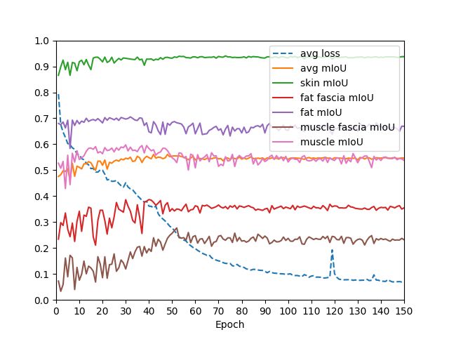
Fig. 1: W-Net model architecture. conv, batchnorm, ReLU max-pool up-conv conv, batchnorm, ReLU
conv, softmax Inset: Loss and mIoU accuracy vs Epoch.
Feature Engineering The RF images of the two patients were of different dimensions (784x192 and
592x192). Since the CNN architecture is limited to fixed-size input, we zero-padded the smaller labeled
and grey images at the bottom to match the input size. To minimize the introduction of phase artifacts
when padding the RF images, shorter RF images were mirrored and reflected at the deepest zero crossing
of each A-scan to avoid waveform discontinuities, to fill in padding values. Our training and testing error
metrics treated the padded region as a special-purpose background in the segmentation task and excluded
the region from the loss function while training the neural network.
Implementation The network is implemented with PyTorch and trained with an Adam optimizer to
optimize over Cross-entropy loss. A batch size of 4 is used for Gradient update computation. Batch
normalization is used. Due to the small size of our augmented training dataset, which allowed fewer
learnable parameters, the number of kernels in each layer for all the models was reduced by a factor of
4 compared to traditional U-Net.
Metrics Mean Intersection over Union (mIoU) and pixel-wise accuracy were the primary metrics used.
We calculated mIoU per segmentation category and mean mIoU across all segmentation categories. Since
some of the test images (8) did not contain all the tissue classes, we stacked all the test images horizontally
and calculated the mean mIoU values reported in Tables 1 & 2.
3 Experiment-1: Tissue Segmentation
We compare W-Net’s performance against Attention U-Net (AU-Net) [18] and the traditional U-Net [19]
architectures. For the U-Net and AU-Net, we analyze with two combinations of inputs, one with single-
channel grey image, the other with a second channel containing RF data. Table 1 depicts the mean
and standard deviation of segmentation pixel-wise and mIoU scores obtained by evaluating on sevenindependently trained models. The scores were calculated on 25 test images augmented with horizontal
flipping. The segmentation results are shown in Fig. 2. Our W-Net better delineates boundaries between
fat and muscle as compared with U-Net and AU-Net.
grey RF label U-Net U-Net AU-Net AU-Net W-Net
with RF with RF uses RF
patient-A
patient-A
patient-B
patient-B
Fig. 2: Segmentation results on four test images with input grey and RF images ( false-color +ve/–ve heat map).
Labels: skin fat fat fascia muscle muscle fascia
Results/Discussions Our model performs better across all tissues classes (except skin), achieving
increased mIoU accuracy (averaged across all tissue classes) by 4.5% and 4.9% compared to regular U-
Net and AU-Net respectively. For muscle fascia, an improvement of 13% and 16% vs U-Net and AU-Net
respectively is observed. Additionally, the U-Net and AU-Net perform better when the RF data is also
provided as an input, indicating that incorporation of RF data boosts segmentation accuracy.
Table 1: Segmentation Pixel-wise and mIoU scores averaged over 7 independent trials
Pixel-wise mIoU
CNN Input data
Acc mean Skin Fat fascia Fat Muscle fasica Muscle
U-Net grey 0.746±0.011 0.555±0.007 0.923±0.002 0.361±0.015 0.699±0.017 0.186±0.013 0.605±0.016
U-Net grey+RF 0.755±0.008 0.565±0.006 0.926±0.002 0.357±0.015 0.706±0.010 0.179±0.009 0.657±0.015
AU-Net grey 0.741±0.015 0.553±0.010 0.924±0.004 0.371±0.017 0.689±0.018 0.181±0.017 0.601±0.020
AU-Net grey+RF 0.740±0.013 0.555±0.007 0.927±0.004 0.355±0.013 0.688±0.015 0.179±0.017 0.627±0.018
W-Net grey+RF 0.769±0.007 0.580±0.005 0.925±0.003 0.373±0.014 0.722±0.009 0.210±0.018 0.669±0.011
4 Experiment-2: Muscle Fascia Analysis
The segmentation accuracy (mIoU) for the tissue classes is visualized with respect to training epochs
(see Fig. 1). We observe that most of the learning for the skin, fat, and muscle tissue classes take place in
the first 20 epochs after which their values converge. The learning for the fat fascia continues until epoch
40 and for the muscle fascia the learning plateaus around epoch 55. As can be observed (refer Table 1),
muscle fascia and fat fascia/stroma have the lowest mIoU accuracy values as compared to other tissue
classes. We can infer that the muscle fascia and fat fascia tissue classes are more difficult to learn as
compared to other tissues classes, with muscle fascia being the most difficult class to learn.We conduct an experiment wherein the augmented training dataset size is gradually increased and
calculate the W-Net segmentation scores on a fixed validation dataset. Results are tabulated in Table 2,
which depicts the mIoU accuracy value for the tissue classes with varying dataset sizes.
Table 2: mIoU accuracy with varying augmented training dataset size.
Augmented Training Pixel-wise mIoU
Dataset Size Acc mean Skin Fat fascia Fat Muscle fasica Muscle
360 0.737 0.547 0.914 0.357 0.688 0.217 0.559
480 0.740 0.557 0.931 0.364 0.689 0.229 0.568
600 0.739 0.563 0.929 0.375 0.681 0.265 0.566
Results/Discussions We can see that from Table 2 adding more data improves the overall accuracy.
With an increase in the augmented training dataset size from 360 to 600 train images, we observe the
mIoU accuracy increases by 22% and 5% for muscle fascia and fat fascia/stroma respectively, while
no significant increase in the mIoU accuracy for the skin, fat, and muscle tissue classes is observed.
One possible conclusion would be that having more training images can help improve the segmentation
accuracy of muscle fascia and fat fascia/stroma. Another possible reason for the poor segmentation
performance of muscle fascia and muscle as compared to fat fascia/stroma and fat could be the loss of
resolution in the ultrasound image as these tissues are anatomically deeper.
5 Conclusion
To the best of our knowledge, this is the first dense semantic segmentation CNN for ultrasound that
attempts to label every pixel, without making use of a background label. This work is also believed to
be the first application of deep learning to shallow subcutaneous ultrasound, which seeks to differentiate
fascia from fat from muscle. Finally, we believe this to be the first work that uses RF (possibly any
waveform) data for segmentation using deep learning techniques.
We presented a novel RF encoding branch to augment models used for ultrasound image segmentation
and demonstrated the improvement in segmentation accuracy across all tissue classes by using RF data.
We compared segmentation accuracy of our W-net against U-Net and AU-Net on our unique dataset.
From the experiments we carried out, our W-Net achieves the best overall mIoU score and the best
individual mIoU scores for muscle fascia and fat fascia/stroma (our most challenging tissue for which all
methods performed the worst).
This being the first segmentation attempt in the SubQ area and considering the small dataset used
for training, the results are on par with the accuracy achieved during the early stage of research in
other prominent areas [8] [11] [13]. Although the results do not yet qualify for practical applications or
real-world deployment of the system in its current state, we have shown that RF data can help with
segmentation and warrants more research in this field. Commercialization opportunities are presently
being pursued and patents are pending.
We plan on expanding the dataset to include scans from different patients under various scan settings.
We hope to develop better data augmentation and labeling techniques. We will explore combinations with
complimentary Neural Network architectures such as GANs [9] and LSTM [3], whose use in segmentation
tasks have gained popularity. Finally, we will explore the utility of W-Net for other segmentation tasks
involving vessels, ligaments, and needles.
Acknowledgements We would like to thank Clarius, the portable ultrasound company, for their ex-
tended cooperation with us. We thank Dr. J. William Futrell and Dr. Ricardo Luis Rodriguez for their
generous computer donation. This work used the Extreme Science and Engineering Discovery Environ-
ment (XSEDE) [20] BRIDGES GPU AI compute resources at the Pittsburgh Supercomputing Center
(PSC) through allocation TG-IRI200003, which is supported by National Science Foundation grant num-
ber ACI-1548562.References
1. Akeret, J., Chang, C., Lucchi, A., Refregier, A.: Radio frequency interference mitigation using deep convo-
lutional neural networks. Astronomy and computing 18, 35–39 (2017)
2. Anderson, P., He, X., Buehler, C., Teney, D., Johnson, M., Gould, S., Zhang, L.: Bottom-up and top-down
attention for image captioning and VQA. CoRR abs/1707.07998 (2017), http://arxiv.org/abs/1707.
07998
3. Azizi, S., Bayat, S., Yan, P., Tahmasebi, A., Kwak, J.T., Xu, S., Turkbey, B., Choyke, P., Pinto, P., Wood,
B., Mousavi, P., Abolmaesumi, P.: Deep recurrent neural networks for prostate cancer detection: Analysis
of temporal enhanced ultrasound. IEEE Transactions on Medical Imaging 37(12), 2695–2703 (Dec 2018).
https://doi.org/10.1109/TMI.2018.2849959
4. Bahdanau, D., Cho, K., Bengio, Y.: Neural machine translation by jointly learning to align and translate.
CoRR abs/1409.0473 (2014)
5. Chen, H., Zheng, Y., Park, J.H., Heng, P.A., Zhou, S.K.: Iterative multi-domain regularized deep learning
for anatomical structure detection and segmentation from ultrasound images. In: Ourselin, S., Joskowicz, L.,
Sabuncu, M.R., Unal, G., Wells, W. (eds.) Medical Image Computing and Computer-Assisted Intervention
– MICCAI 2016. pp. 487–495. Springer International Publishing, Cham (2016)
6. Dolz, J., Gopinath, K., Yuan, J., Lombaert, H., Desrosiers, C., Ben Ayed, I.: Hyperdense-net: A hyper-
densely connected cnn for multi-modal image segmentation. IEEE Transactions on Medical Imaging 38(5),
1116–1126 (2019)
7. Dolz, J., Desrosiers, C., Ben Ayed, I.: Ivd-net: Intervertebral disc localization and segmentation in mri with
a multi-modal unet. In: Zheng, G., Belavy, D., Cai, Y., Li, S. (eds.) Computational Methods and Clinical
Applications for Spine Imaging. pp. 130–143. Springer International Publishing, Cham (2019)
8. Girshick, R.B., Donahue, J., Darrell, T., Malik, J.: Rich feature hierarchies for accurate object detection and
semantic segmentation. CoRR abs/1311.2524 (2013), http://arxiv.org/abs/1311.2524
9. Goodfellow, I.J., Pouget-Abadie, J., Mirza, M., Xu, B., Warde-Farley, D., Ozair, S., Courville, A., Bengio,
Y.: Generative adversarial networks (2014)
10. Gorce, J.M., Friboulet, D., Dydenko, I., D’hooge, J., Bijnens, B., Magnin, I.: Processing radio frequency
ultrasound images: A robust method for local spectral features estimation by a spatially constrained para-
metric approach. IEEE transactions on ultrasonics, ferroelectrics, and frequency control 49, 1704–19 (01
2003). https://doi.org/10.1109/TUFFC.2002.1159848
11. Hariharan, B., Arbelaez, P., Girshick, R.B., Malik, J.: Simultaneous detection and segmentation. CoRR
abs/1407.1808 (2014), http://arxiv.org/abs/1407.1808
12. Khened, M., Varghese, A., Krishnamurthi, G.: Fully convolutional multi-scale residual densenets for cardiac
segmentation and automated cardiac diagnosis using ensemble of classifiers. CoRR abs/1801.05173 (2018),
http://arxiv.org/abs/1801.05173
13. Long, J., Shelhamer, E., Darrell, T.: Fully convolutional networks for semantic segmentation. In: 2015
IEEE Conference on Computer Vision and Pattern Recognition (CVPR). pp. 3431–3440 (June 2015).
https://doi.org/10.1109/CVPR.2015.7298965
14. Mendizabal-Ruiz, E.G., Biros, G., Kakadiaris, I.A.: An inverse scattering algorithm for the segmentation
of the luminal border on intravascular ultrasound data. In: Yang, G.Z., Hawkes, D., Rueckert, D., Noble,
A., Taylor, C. (eds.) Medical Image Computing and Computer-Assisted Intervention – MICCAI 2009. pp.
885–892. Springer Berlin Heidelberg, Berlin, Heidelberg (2009)
15. Mishra, D., Chaudhury, S., Sarkar, M., Manohar, S., Soin, A.S.: Segmentation of vascular regions in ul-
trasound images: A deep learning approach. 2018 IEEE International Symposium on Circuits and Systems
(ISCAS) pp. 1–5 (2018)
16. Mishra, D., Chaudhury, S., Sarkar, M., Soin, A.: Ultrasound image segmentation: A deeply supervised net-
work with attention to boundaries. IEEE Transactions on Biomedical Engineering PP, 1–1 (10 2018).
https://doi.org/10.1109/TBME.2018.2877577
17. Noble, A., Boukerroui, D.: Ultrasound image segmentation: a survey. IEEE Transactions on Medical Imaging
25(8), 987–1010 (Aug 2006), https://hal.archives-ouvertes.fr/hal-00338658
18. Oktay, O., Schlemper, J., Folgoc, L., Lee, M., Heinrich, M., Misawa, K., Mori, K., McDonagh, S., Hammerla,
N., Kainz, B., Glocker, B., Rueckert, D.: Attention u-net: Learning where to look for the pancreas (04 2018)
19. Ronneberger, O., Fischer, P., Brox, T.: U-net: Convolutional networks for biomedical image segmentation. In:
Navab, N., Hornegger, J., Wells, W.M., Frangi, A.F. (eds.) Medical Image Computing and Computer-Assisted
Intervention – MICCAI 2015. pp. 234–241. Springer International Publishing, Cham (2015)
20. Towns, J., Cockerill, T., Dahan, M., Foster, I., Gaither, K., Grimshaw, A., Hazlewood, V., Lathrop, S., Lifka,
D., Peterson, G.D., Roskies, R., Scott, J.R., Wilkins-Diehr, N.: Xsede: Accelerating scientific discovery.
Computing in Science & Engineering 16(5), 62–74 (Sept-Oct 2014). https://doi.org/10.1109/MCSE.2014.80,
doi.ieeecomputersociety.org/10.1109/MCSE.2014.80
21. Vaswani, A., Shazeer, N., Parmar, N., Uszkoreit, J., Jones, L., Gomez, A.N., Kaiser, L.u., Polosukhin, I.:
Attention is all you need. In: Guyon, I., Luxburg, U.V., Bengio, S., Wallach, H., Fergus, R., Vishwanathan, S.,
Garnett, R. (eds.) Advances in Neural Information Processing Systems 30, pp. 5998–6008. Curran Associates,
Inc. (2017), http://papers.nips.cc/paper/7181-attention-is-all-you-need.pdf22. Wang, P., Patel, V.M., Hacihaliloglu, I.: Simultaneous segmentation and classification of bone surfaces from
ultrasound using a multi-feature guided cnn. In: Frangi, A.F., Schnabel, J.A., Davatzikos, C., Alberola-López,
C., Fichtinger, G. (eds.) Medical Image Computing and Computer Assisted Intervention – MICCAI 2018.
pp. 134–142. Springer International Publishing, Cham (2018)
23. Wu, L., Xin, Y., Li, S., Wang, T., Heng, P., Ni, D.: Cascaded fully convolutional networks for automatic pre-
natal ultrasound image segmentation. In: 2017 IEEE 14th International Symposium on Biomedical Imaging
(ISBI 2017). pp. 663–666 (April 2017). https://doi.org/10.1109/ISBI.2017.7950607
24. Yoon, Y.H., Khan, S., Huh, J., Ye, J.C.: Efficient b-mode ultrasound image reconstruction from sub-
sampled rf data using deep learning. IEEE Transactions on Medical Imaging 38(2), 325–336 (Feb 2019).
https://doi.org/10.1109/TMI.2018.2864821
Supplementary Material
grey RF label W-Net grey
W-Net RF 7x3 W-Net RF 11x3 W-Net RF 21x5 W-Net RF 51x9
U-Net U-Net with RF AU-Net AU-Net with RF
Fig. 3: Activation maps of the first convolutional block overlaid on top of the input grey image along
with input grey, RF and label images. We can see that the W-Net grey branch activation map is noise
free as compared to other CNN networks. We can observe that the W-Net’s grey branch activation map
is responding to skin and fascias while the RF kernel branches are responding more to particular features.
Like, RF 7x3 is responding to the skin and RF 21x5 to the fat and muscle boundary region.grey RF label
conv1 grey conv1 RF 7x3 conv1 RF 11x3 conv1 RF 21x5 conv1 RF 51x9
conv2 grey conv2 RF 7x3 conv2 RF 11x3 conv2 RF 21x5 conv2 RF 51x9
conv3 grey conv3 RF 7x3 conv3 RF 11x3 conv3 RF 21x5 conv3 RF 51x9
conv4 grey conv4 RF 7x3 conv4 RF 11x3 conv4 RF 21x5 conv4 RF 51x9
Fig. 4: W-Net’s activation maps of the various convolutional blocks overlaid on top of the input grey
image along with input grey, RF and label images. We observe that larger RF kernels are responding to
more grouped regions compared to smaller RF kernels.You can also read