Wave Turbulence, Zonal Jets and Staircase Patterns in Fluids and Plasmas

Wave Turbulence, Zonal Jets
 and Staircase Patterns in
 Fluids and Plasmas
 P.H. Diamond
 U. C. San Diego

 Physics Colloquium: IIT, Delhi
 March 22, 2021

This research was supported by the U.S. Department of Energy, Office of Science, Office
of Fusion Energy Sciences, under Award Number DEFG02-04ER54738.

Outline
• Primer in Confinement: Pipes and Donuts

 The problem of scales

• Scale Selection I
 – Shear flow effects

 – Constructing models potential vorticity (GFD and Plasma)

 – Physics of zonal flows

 – Closing the feedback loop: predator-prey analogue

• Scale Selection II – the ExB staircase
 – Staircases

 – Model-Bistable mixing

 – Some results

• Open Issues and Current Research

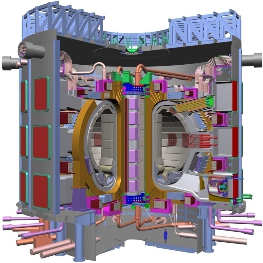
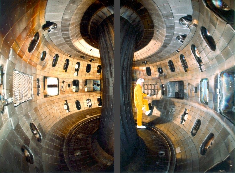
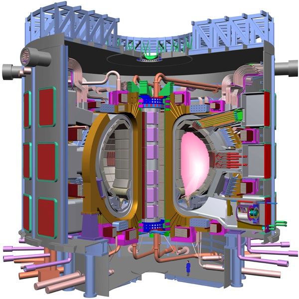
Magnetically confined plasma tokamaks
• Nuclear fusion: option for generating large
 amounts of carbon-free energy – “30 years in the
 future and always will be… “
• Challenge: ignition -- reaction release more energy
 than the input energy
 Lawson criterion: DIII-D

 confinement ∼
 
 turbulent transport
• Turbulence: instabilities and collective oscillations
 low frequency modes dominate the
 transport ( < Ω )

• Key problem: Confinement, especially scaling
• NB: Not the only problem 3
 ITER

A Simpler Problem:
Drag in Turbulent Pipe Flow

• Essence of confinement problem:
 – given device, sources; what profile is achieved?

 – = / in , How optimize W, stored energy

• Related problem: Pipe flow drag ↔ momentum flux

 Δ pressure drop

 a Turbulent
 
 Δ 2 = ∗2 2 Laminar

 friction velocity V∗ ↔ 
Balance: momentum transport to wall 
(Reynolds stress) vs Δ 2 Δ / 
 =
 (1/2) 2
 Flow velocity profile Friction factor

(Core)
 
 inertial sublayer ~ logarithmic (~ universal)

 viscous sublayer (linear)
 0 • Problem: physics of ~ universal
 logarithmic profile?
 • Universality scale invariance
 Wall

• Prandtl Mixing Length Theory (1932)
 ∗ Spatial counterpart
 – Wall stress = ∗2 = − / or: ~
 of K41
 eddy viscosity
 Scale of velocity gradient?
 – Absence of characteristic scale
 ∼ ∗ ≡ mixing length, distance from wall
 ∼ ∗ ln( / 0 ) Analogy with kinetic theory …

 = → 0 , viscous layer 0 = / ∗

Some key elements:
• Momentum flux driven process ↔ contrast fixed profile

• Turbulent diffusion model of transport - eddy viscosity

• Mixing length – scale selection

 ~ macroscopic, eddys span system 0 < < 

 ~ flat profile – strong mixing

• Self-similarity x ↔ no scale, within 0 , 

• Reduce drag by creation of buffer layer i.e. steeper gradient than

 inertial sublayer (due polymer) – enhanced momentum confinement

 [N.B. : Analogue of H-mode]

Without vs With Polymers
Comparison NYFD 1969

Turbulence in Tokamaks
 A Primer

Primer on Turbulence in Tokamaks I
• Strongly magnetized
 0
 – Quasi 2D cells, Low Rossby # 

 * – Localized by ⋅ = 0 (resonance) – pinned cells
 
 ⊥ �
• ⊥ = + × ,̂ ~ 0 ≪ 1
 Ω 
 
• , , driven

• Akin to thermal convection with: g magnetic curvature

• Re ≈ / ill defined, not representative of dynamics

• Resembles ‘wave turbulence’, not high Navier-Stokes turbulence
 � /Δ ∼ 1
• ∼ Kubo # ≈ 1

• Broad dynamic range, due electron and ion scales, i.e. , , 

Primer on Turbulence in Tokamaks II

 • Characteristic scale ~ few “mixing

 length”
 
 • Characteristic velocity ~ ∗ 
 
 • Transport scaling: ~ ∼ ∗ - Gyro-Bohm
Key:
 ∼ ∼ / - Bohm
2 scales:
 • i.e. Bigger is better! sets profile scale via heat
 ≡ gyro-radius
 balance (Why ITER is huge…)
 ≡ cross-section
 ∗ ≡ / key ratio • Reality: ~ ∗ , < 1 ‘Gyro-Bohm breaking’
 ∗ ≪ 1 • 2 Scales, ∗ ≪ 1 key contrast to pipe flow

THE Question ↔ Scale Selection
• Expectation (from pipe flow):

 – ∼ 

 – ∼ 

• Hope (mode scales)
 – ∼ 

 – ∼ ∼ ∗ 

• Reality: ∼ ∗ , < 1

 Why? What physics competition sets ?

Scale Selection

Zonal Flow Jets Natural to Planets, Tokamaks
• Zonal Flows Ubiquitous for: � < 1
 R0 ≡ Rossby # = /
 ~ 2D fluids / plasmas R0 < 1
 Rotation Ω , Magnetization B0 , Stratification
 Ex: MFE devices, giant planets, stars…

 Solar Tachocline
 Sheared Flow

 14

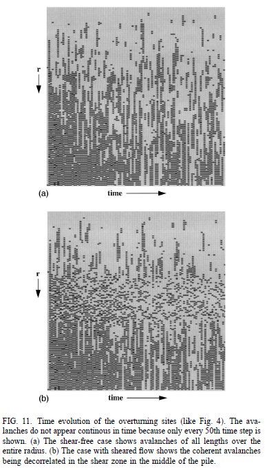
Shear Flows – Significance?
 • How is transport affected by shear flows ?

 shear decorrelation!
No
shear • Back to sandpile model:
 2D pile +
 sheared flow of
 grains
shear

 Shearing flow
 decorrelates
 Toppling sequence

 • Avalanche coherence destroyed by shear flow

rule correction
 + decorrelation
• Implications:

 Spectrum of Avalanches decorrelation

N.B.
- Profile steepens for unchanged toppling
 rules
- Distribution of avalanches changed

How, Why Do Flows Form?
Models and Potential Vorticity

Flows
• GFD The Fluid Dynamics of Potential Vorticity (R. Salmon)

• Ditto for confined plasmas... (PD)

• What is PV ?
 – Consider freezing-in:
 ⃗2
 ⃗
 = ⃗2 − ⃗1 = ⃗ ⋅ [ ⃗ “frozen in” to flow ]
 
 ⃗1

 – Flow ↔ Vorticity = × 

 + ⋅ = − − 2Ω × 
 
 Coriolis / Lorentz

PV cont’d
• Then, for = :

 + 2Ω = × × + 2Ω

 +2Ω +2Ω
 = ⋅ 
 
 ⃗ +2Ω
 
 = ⃗ ⋅ → 
 “frozen in”

 → non-trivial frozen in ≠ passive !

• Passive Scalar 
 ⃗2
 
 =0
 
 ⃗1
 ⃗
 
 ⇒ =0 ; = ⋅ ⃗
 

PV cont’d
 
 ⋅ ⃗ = 0
 
 but ⃗ = ⃗ ⋅ 
 
 d +2Ω +2Ω
 = ⋅ , so
 dt 

• + 2Ω ⋅ =0 statement of PV conservation
 
 +2Ω
• = = ⋅ { Good analogy with conserved charge }
 

PV Conservation ↔ Trade-offs
 + 2Ω
 = ⋅ 
 
• displace latitude changes

• displace in density changes

 thickness

 etc.

PV cont’d
• Conservation ↔ Symmetry ? - ala’ Noether

 Particle re-labeling; ⃗ , → ′ = + 
 [PV conserved when particles can be re-labeled, without changing the
 thermodynamic state]

• Related: Kelvin’s Theorem ( = const. = ( ))

 ∫ ⃗ ⋅ + 2Ω =0
 
 total circulation conserved (parcel + planetary)

From Kelvin’s Theorem to the Plane Model (Charney)
 - Kelvin’s Theorem for rotating system

 relative planetary

 - → geostrophic balance

 → 2D dynamics

 - Displacement on beta plane

 →

 So...

Charney Equation, cont’d

 - Charney equation
 n.b. topography
 - Locally Conserved PV
 parcel planetary
 - Latitudinal displacement → change in relative
 vorticity
 - Linear consequence → Rossby Wave

 = 0 zonal flow
 = 0 azimuthal symmetry
 observe:
 → Rossby wave intimately connected to momentum transport
 Reynolds stress ⟨ ⟩
 - Latitudinal PV Flux → circulation

PV Dynamics – Plasmas ?
• Isn’t this about plasmas, too?
 2Ω → Ω ̂
 
• = + 2Ω ⋅ now → 0 + �
 
 → ̂
 +Ω 
 So =0 ala’ Geostrophic:
 0 + �

 � 
 1 = − × ̂
 ⇒ 
 � − Ω =0 
 0 

 2
 � � �
 = 
 with ≪ < ~ ~ 0
 ∥ 0 0 

 � � �
 Hasegawa-Mima Eqn.
 
 − 2 ⊥2 + ∗ =0 PV conservation
 

PV and Models - Plasmas
• Hasegawa-Mima, prototype:

 − 2 2 + ln 0 ( ) = 0
 
• tip of iceberg of zoology of systems

• captures essence

• in tokamak, zonal flows have: ∥ = 0 and = 0

 2 = 0
 
 generation of flow � 2 � vorticity flux

Physics of Zonal Flows

How do Zonal Flow Form?
Simple Example: Zonally Averaged Mid-Latitude Circulation

 Rossby Wave:

 = − 2
 ⊥2 v~y v~x = ∑ − k x k y φˆk
 k
 2
 = 2 2 2
 , � � = ∑ − � 
 ⊥

 ∴ < 0 Backward wave!
 Momentum convergence
 at stirring location

Some similarity to spinodal decomposition phenomena
 Both ‘negative diffusion’ phenomena Cahn-Hillard Equation

Wave-Flows in Plasmas
 MFE perspective on Wave Transport in DW Turbulence
 • localized source/instability drive intrinsic to drift wave structure
 – couple to damping ↔ outgoing wave
 x
 x Emission
 Absorption
 x
 x x x x
 x x
 x x > 0 ⇒ v gr > 0
 x x kθ k r v*
 x x x – v gr = −2 ρ
 2
 x < 0 ⇒ v gr < 0
Fluctuations x=0
 s
 (1 + k ⊥2 ρ s2 ) 2
Pinned to non-resonant c2 v* < 0 ⇒ kr kθ > 0
 radial structure vrE vθE = − 2 | φk |2 k r kθ < 0
surfaces B

 • outgoing wave energy flux → incoming wave momentum flux
 → counter flow spin-up!
 vgr vgr

 • zonal flow layers form at excitation regions
30

Plasma Zonal Flows I
• What is a Zonal Flow? – Description?
 – n = 0 potential mode; m = 0 (ZFZF), with possible sideband (GAM)
 – toroidally, poloidally symmetric ExB shear flow

• Why are Z.F.’s important?
 – Zonal flows are secondary (nonlinearly driven):
 • modes of minimal inertia (Hasegawa et. al.; Sagdeev, et. al. ‘78)
 • modes of minimal damping (Rosenbluth, Hinton ‘98)
 • drive zero transport (n = 0)

 – natural predators to feed off and retain energy released by
 gradient-driven microturbulence
i.e. ZF’s soak up turbulence energy

Plasma Zonal Flows II
• Fundamental Idea:
 – Potential vorticity transport + 1 direction of translation symmetry
 → Zonal flow in magnetized plasma / QG fluid
 – Kelvin’s theorem is ultimate foundation

• Charge Balance → polarization charge flux → Reynolds force
 – Polarization charge − ρ 2∇ 2φ = ni ,GC (φ ) − ne (φ )
 polarization length scale ion GC electron density
 ~
 – so Γi ,GC ≠ Γe ρ 2 v~rE ∇ ⊥2 φ ≠ 0 ‘PV transport’
 polarization flux → What sets cross-phase?
 – If 1 direction of symmetry (or near symmetry):
 ~
 − ρ 2 v~rE ∇ 2⊥φ = −∂ r v~rE v~⊥ E (Taylor, 1915)

 − ∂ r v~rE v~⊥ E Reynolds force Flow Recall ⟨ ⟩ evolution!

Zonal Flows Shear Eddys I
• Coherent shearing: (Kelvin, G.I. Taylor, Dupree’66, BDT‘90)
 – radial scattering + VE ' → hybrid decorrelation
 – k r2 D⊥ → (kθ2 VE '2 D⊥ / 3)1/ 3 = 1 / τ c
 shearing restricts mixing scale!

• Other shearing effects (linear): Response shift
 and dispersion
 – spatial resonance dispersion: ω − k||v|| ⇒ ω − k||v|| − kθ VE ' (r − r0 )
 – differential response rotation → especially for kinetic curvature
 effects

Quasi-Particle Model – Eddy Population Evolution
 • Zonal Shears: Wave kinetics (Zakharov et. al.; P.D. et. al. ‘98, et. seq.)
 Coherent interaction approach (L. Chen et. al.)
 ~
 • dk r / dt = −∂ (ω + kθ VE ) / ∂r ; VE = VE + VE
 Mean
 : k r = k r( 0 ) − kθ VE′τ
 shearing

 Zonal : δk r = Dkτ
 2

 Random
 ~ 2
 shearing Dk = ∑
 kθ2 VE′,q
 q
 τ k ,q - Wave ray chaos (not shear RPA)
 underlies Dk → induced diffusion
 • Mean Field Wave Kinetics
 - Induces wave packet dispersion
 ∂N ∂ ∂N
 + (Vgr + V ) ⋅ ∇N − (ω + kθ VE ) ⋅ = γ k N − C{N }
 ∂t ∂r ∂k - Applicable to ZFs and GAMs
 ∂ ∂ ∂
 ⇒ N − Dk N = γ k N − C{N } Zonal shearing
 ∂t ∂k r ∂k r

 Evolves population in response to shearing

Closing the Feedback Loop
 Predator-Prey Analogue

Energetics
• Energetics: Books must Balance for Reynolds Stress-Driven Flows!

• Fluctuation Energy Evolution – Z.F. shearing

 ∂ ∂ ∂ ∂ ∂ − 2k r kθ V* ρ s2
 ∫ dk ω ∂t
 N −
 ∂k r
 Dk
 ∂k r
 N ⇒
 ∂t
 ε = − ∫ dk Vgr (k ) Dk
 ∂k r
 N Vgr =
 (1 + k 2
 ρ s2 )
 2
 ⊥

 Point: For d Ω / dk r < 0, Z.F. shearing damps wave energy

• Fate of the Energy: Reynolds work on Zonal Flow !
 (~~
 )
 Modulational ∂ t δVθ + ∂ δ VrVθ / ∂r = γδVθ
 Instability ~~ k r k θ δN N.B.: Wave decorrelation essential:
 δ VrVθ ~ Equivalent to PV transport
 (1 + k⊥2 ρ s2 ) 2
• Bottom Line: (c.f. Gurcan et. al. 2010)

 – Z.F. growth due to shearing of waves

 – “Reynolds work” and “flow shearing” as relabeling → books balance

 – Z.F. damping emerges as critical; MNR ‘97

Feedback Loops
• Closing the loop of shearing and Reynolds work

• Spectral ‘Predator-Prey’ Model

 Prey → Drift waves, 
 ∂ ∂ ∂ ∆ωk 2
 N − Dk N =γk N − N
 ∂t ∂k r ∂k r N0

 Predator → Zonal flow, |ϕq|2
 ∂ ∂ N
 | φq |2 = Γq | φq |2 −γ d | φq |2 −γ NL [| φq |2 ] | φq |2
 ∂t ∂k r
 Self-regulating system “ecology”
 Mixing scale regulated

Feedback Loops II
• Recovering the ‘dual cascade’:
 ⇒ Analogous → forward potential
 – Prey → ~ ⇒ induced diffusion to high kr
 enstrophy cascade; PV transport

 ⇒ growth of n=0, m=0 Z.F. by turbulent Reynolds work
 Predator → | φq | ~ VE ,θ
 2 2
 –
 ⇒ Analogous → inverse energy cascade

 System Status

• Mean Field Predator-Prey Model

 (P.D. et. al. ’94, DI2H ‘05)
 ∂
 N = γN − αV 2 N − ∆ωN 2
 ∂t
 ∂ 2
 V = αNV 2 − γ dV 2 − γ NL (V 2 )V 2
 ∂t

Scale Selection II
– the ExB Staircase
 Spatial Structure due
Closed Feedback Loops

Dynamics in Real Space
• Conventional Wisdom Homogenization ?!

 – Prandtl, Batchelor, Rhines: (2D fluid)

 – PV homogenized:
 Shear + Diffusion → 0
 1/3
 – Mechanism: - Shear dispersion ∼ 

 - Forward Enstrophy Cascade, ‘PV Mixing’

 – Introduce Bi-stable Mixing Layers

 – Cahn-Hilliard + Eddy Flow bistability (Fan, P.D., Chacon,
 PRE Rap. Com. ‘17)
 target pattern

Fate of Gradient?
 localized
 QL inhomogeneous
 mixing
 OR

 OR - ‘staircase’

 - layers, steps, corrugations
 pattern of - shear layers relation to corrugations?
 inhomogeneous
 mixing ?!
 ?

 Zonal flows at corrugations ?

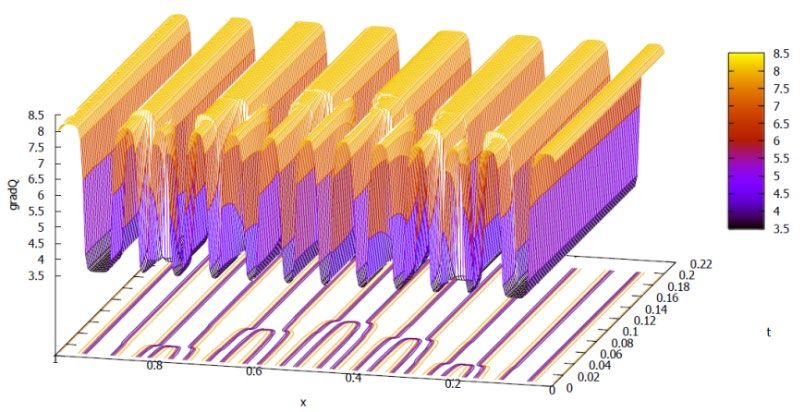
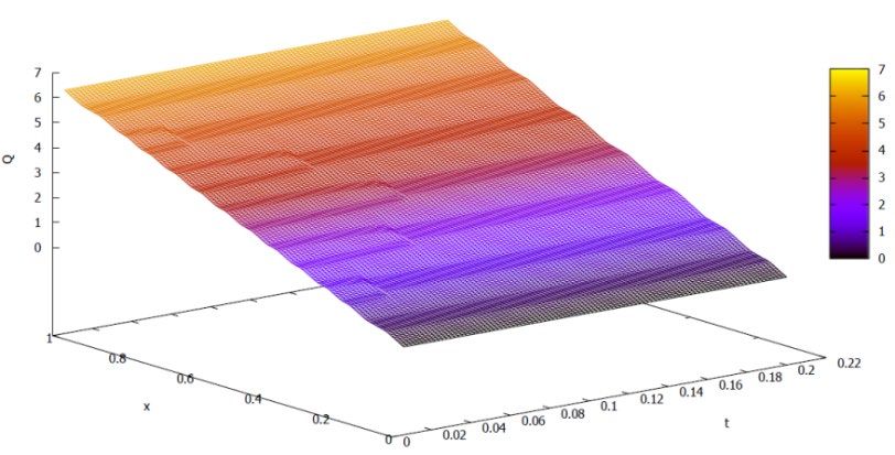
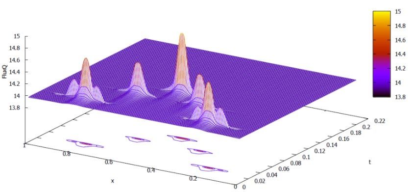
Spatial Structure: ExB staircase formation
• ExB flows often observed to self-organize structured pattern
 in magnetized plasmas
• `ExB staircase’ is observed to form (G. Dif-Pradalier, P.D. et al. Phys. Rev. E. ’10)

 - flux driven, full f simulation

 - Quasi-regular pattern of shear layers
 and profile corrugations (steps)

 - Region of the extent
 interspersed by temp. corrugation/ExB jets

 → ExB staircases

 - so-named after the analogy to PV staircases
 and atmospheric jets

 - Step spacing avalanche distribution
 outer-scale
 also: GK5D, Kyoto-Dalian-SWIP group, - scale selection problem
 gKPSP, ... several GF codes

ExB Staircase, cont’d
• Important feature: co-existence of shear flows and avalanches/spreading

 - Seem mutually exclusive ?

 → strong ExB shear prohibits transport

 → mesoscale scattering smooths out corrugations

 - Can co-exist by separating regions into:
 1. avalanches of the size

 2. localized strong corrugations + jets

 • How understand the formation of ExB staircase??
 - What is process of self-organization linking avalanche scale to ExB step scale?

 i.e. how explain the emergence of the step scale ?

 • Some similarity to phase ordering in fluids – spinodal decomposition

Model Bistable Mixing

Basic Equations ↔ Hasegawa-Wakatani (life beyond CHM)
 2
 + ∥ ∥2 − = ⊥2 ⊥2 
 ⊥

 + ∥ ∥2 − = 0 ⊥2 
 
 = + × ̂ ⋅ = + � ⊥2 = ⊥2 + ⊥2 �
 
• PV = − ⊥2 conserved! , to , 0

• ∥ ≠ 0 → � � ≠ 0 ‘negative dissipation drift instability (Sagdeev, et. al.)
 mechanism’
 ≤ ∗ → � � > 0
 shear
• ZF ∥ = 0 ↔ ⊥2 PV exchange

• ZF → � 2 � → Reynolds force
 � 2 �
 ?
 Corrugation → � � → particle flux c.f. singh, P.D. 2021

‘Bistable’ Mixing – A Simple Mechanism
• Mean field model with 2 mixing scales (after BLY 1998)

• So, for H-W:

• Density: simple mixing + 2 length scale
 staircase
• Vorticity:

• Enstrophy(intensity): includes crude turbulence
 spreading model
• � 
 , ∼ 
 0 excitation scale (drive)
 Rhines scale (emergent)
 vs Δ - can be generalized
• Scale cross-over ‘transport bifurcation’

• 0 / < 1 → strong mixing (eddys) two scales!

• 0 / > 1 → weak mixing (waves) sharpening feedback

• Is this ~ equivalent to ‘two-fluid’ mixing length model (E.A. Spiegel)

How, Why ?
• PV is mixed natural for ‘mixing length model’ exploits conserved phase space density

• Potential Enstrophy is natural formulation − ⟨ 2 ⟩ for intensity conserved

• Beyond BLY 2 mean fields , ⟨ 2 ⟩ + – fluctuation potential enstrophy

 exchange and couplings

• Reynolds work and particle flux couple mean and fluctuations

• Nonlinear damping ↔ forward enstrophy cascade

• , → turbulent transport coefficients are fundamental

• Glorified ‘ − model’

How, Why ? Cont’d
 • > → simplifies inversion ( 2 → )

 • Dissipative DW ~ adiabatic regime: ∥2 
 2
 / ≫ 

 ≈ � 2 / ∼ 2 / → � phase fixed by !

 Major simplification → solid, where applicable

 ~ (non-resonant diffusion)

 • � 2 = − 2 + Π 

 2 = shear on

 • � � 2 → − 2 1/2 spreading, entrainment, SOFT

How, Why ? Cont’d
 • , regulate P.E. exchange between mean, fluctuations key role in model

 0 0
 • Mixing Length: = 2 /2 = 2 /2
 − 2 1+ 02 / 
 1+ 0 

 Physics: “Rossby Wave Elasticity’

 � 2 Δ Δ 
 i.e. ∼ → � 2 ≈ � 2 for Δ < 
 Δ 2 + Δ 2 2

 waves enhance memory

 ~ → nonlinear Γ vs → S-curve

 • Soft point: → suppression exponent

 = 1 doesn't always work

 Rigorous bound, from fundamental equations?

Some Results

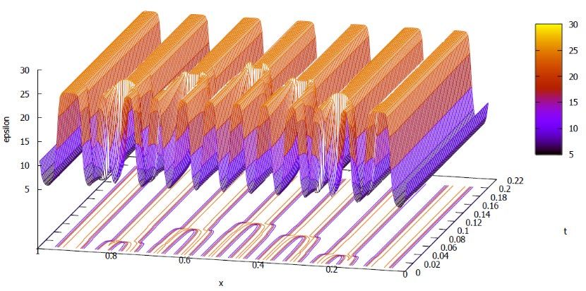
Staircase Model – Formation and Merger (QG-HM)
 Energy 

fluctuations

 mergers

 PV transport
 - - - PV mixing events
 - top - Γ bottom
 Note later staircase mergers induce strong PV flux episodes!
 (Malkov, P.D.; PR Fluids 2018) 51

Staircase are Dynamic Patterns

 t=1300
oShear pattern detaches and delocalizes
from its initial position of formation.

oMesoscale shear lattice moves in the
up-gradient direction. Shear layers
condense and disappear at x=0.
 t=700
oShear lattice propagation takes place
over much longer times. From t~O(10)
to t~(104).

oBarriers in density profile move
upward in an “Escalator-like” motion.

 Macroscopic Profile Re-structuring

 (Ashourvan, P.D. 2016)
 52

FAQ re: Staircase Structure?
• Number of steps? - domain L Scale Selection ?!

• Scan # steps vs at t=0 (n.b. mean gradient)
 – a maximum # steps (and minimal step size) vs 

 – rise: increase in free energy as ↑

 – drop: diffusive dissipation limits 

• Height of steps?
 – minimal height at maximal #

 system has a ‘sweet spot’ for many,

 small steps and zonal layers

Spreading/Entrainment
 • Spreading/entrainment effect on P.E. is unconstrained, beyond ⋅ Γ structure

 Contrast: , Follow standard − model CRUDE !

 • How robust is staircase to effects of entrainment, avalanching… ?

 • → 2 1/2

 Entrainment has significant
 effect on S.C. structure

 Large → wash out S.C.

 • Important !

Mergers Happen !

 • ‘Type-II’ merger (c.f. Balmforth, in ‘Interfaces’)

 • ‘Type-I’ (motion) mergers also observed

 Staircase coarsens….

 Obvious TBD:

 – Interplay/Competition of Spreading and Mergers?

 – Scan coarsening time vs , merger rate vs increments in 

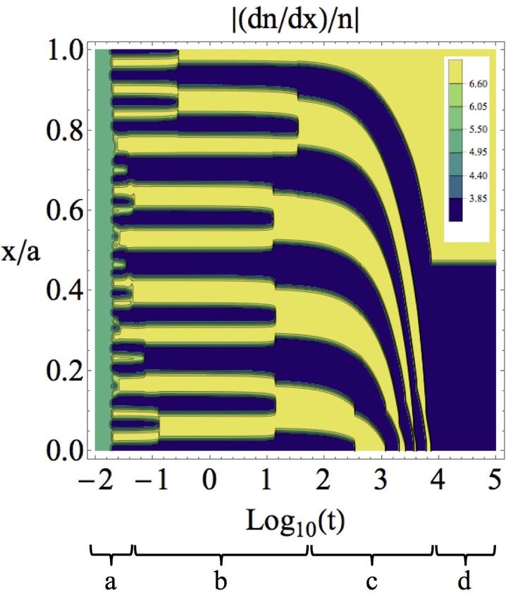
Macro-Barriers via Condensation ∇n

 (a) Fast merger of micro-scale SC. Formation
 of meso-SC.
 (b) Meso-SC coalesce to barriers
 (c) Barriers propagate along gradient, x
 condense at boundaries
 (d) Macro-scale stationary profile

 Shearing field

 u

 Steady
 state
 x d
 c
 b LH transition?
56
 log10 (t) a
 (Ashourvan, P.D. 2016)

Conclusion and
Current Research

Conclusions
• Shear Flows externally and self-generated effective at
 regulating transport via scale and rate selection

• Potential Vorticity and its conservation are powerful formulations for
 GFD and Magnetized Plasma dynamics

• Zonal Flows are self-generated flows of minimum inertia, damping
 and transport and thus are of great interest

• Turbulence, zonal models (and profile corrugations) are a multi-
 state self-regulating system

Conclusions, cont’d
 • Inhomogeneous mixing produces layered domains or

 staircases scale selection

 • Staircase can be recovered via bi-stable mixing model for

 , 2 , emergent length [Rhines scale] is crucial

 • Edge Barriers recovered from hierarchical mergers and

 staircase condensation

Ongoing Research
 • Staircase-avalanche co-existence

 • Staircase “resilience”

 • Heterogeneous staircase profile, ⟨ ⟩ variation

 • Development of coarsening

 • Transitions, especially barriers

 • Self-organized, ~ marginal cells of pinned turbulence

 Rosenbluth ‘87