Where She Blows! A Ten Year Dust Climatology of Western New South Wales Australia - MDPI
←
→
Page content transcription
If your browser does not render page correctly, please read the page content below
geosciences
Article
Where She Blows! A Ten Year Dust Climatology of
Western New South Wales Australia
John Leys 1, *, Craig Strong 2       ID
                                          , Stephan Heidenreich 3 and Terry Koen 4
 1   Office of Environment and Heritage, Science Division, Gunnedah, NSW 2380, Australia
 2   The Fenner School of Environment & Society, The Australian National University,
     Canberra, ACT 2601, Australia; Craig.Strong@anu.edu.au
 3   Office of Environment and Heritage, Science Division, Gunnedah, NSW 2380, Australia;
     Stephan.Heidenreich@environment.nsw.gov.au
 4   Office of Environment and Heritage, Science Division, Cowra, NSW 2794, Australia;
     Terry.Koen@environment.nsw.gov.au
 *   Correspondence: John.leys@environment.nsw.gov.au; Tel.: +61-267-420-2345

 Received: 29 May 2018; Accepted: 16 June 2018; Published: 23 June 2018

 Abstract: Dust emissions contribute significantly to atmospheric processes impacting the functioning of
 various earth and human systems. The question is often asked “how much dust is acceptable?” From a
 land management perspective, the aim is to reduce the degradation effects of wind erosion over time.
 To do this, we need to know the range of dust activity over a long time period and to set a target that
 shows a reduction in dust activity. In this study, dust activity is described by the number of dust hours per
 July to June period (dust storm year, DSY). We used the DustWatch network of high resolution particulate
 matter less than 10 µm (PM10) instruments to characterise the dust climatology for a ten year period
 for western New South Wales (NSW), Australia. The ten year study period covered one of the driest
 and wettest periods in south-eastern Australia, providing confidence that we have measurements of
 extremes of dust (0 to 412 h/DSY), rainfall (98 to 967 mm/DSY), and ground cover (0 to 99% of area/DSY).
 The dust data are then compared to remotely sensed ground cover and measured rainfall data to develop
 targets across a rainfall gradient. Quantile regression was used to estimate the number of dust hours for a
 given DSY rainfall at 21 DustWatch Nodes (DWN). The 75th percentile is used to determine the target
 number of dust hours for a ten year average DSY. The monitoring network clearly identified locations
 of high dust activity and changes in dust and ground cover that are associated with rainfall. The dust
 hour targets for NSW indicated that for every 100 mm increase in DSY rainfall (between 250 and 650 mm)
 there is a 10 h decrease in dust hours. The dust target enables us to evaluate whether wind erosion is
 decreasing with time for sites with different rainfall.

 Keywords: dust storms; climatology; PM10; monitoring; DustWatch

1. Introduction
     Dust emissions can come from natural sources, like the Sahara [1] or anthropogenically modified
sources like the Mallee in Australia or the Great Plains of the United States [2]. Anthropogenic sources
are generally a sign that the land is not being managed within its capacity and the soil resource
is degrading. Understanding where and why dust emissions are changing is fundamental to
implementing better Natural Resource Management programs [3,4]. From a land management
perspective, the aim is to reduce the degradation effects of wind erosion over time. To do this,
we need to know “how much dust is acceptable?” In this context, acceptable is about improvement in
land condition, or a reduction in wind erosion.
     Government environmental reporting programs, such as the State of the Environment reporting
in Australia [5–7], State and Outlook Report from the European Union (EU) [8], and the Report on the

Geosciences 2018, 8, 232; doi:10.3390/geosciences8070232                      www.mdpi.com/journal/geosciences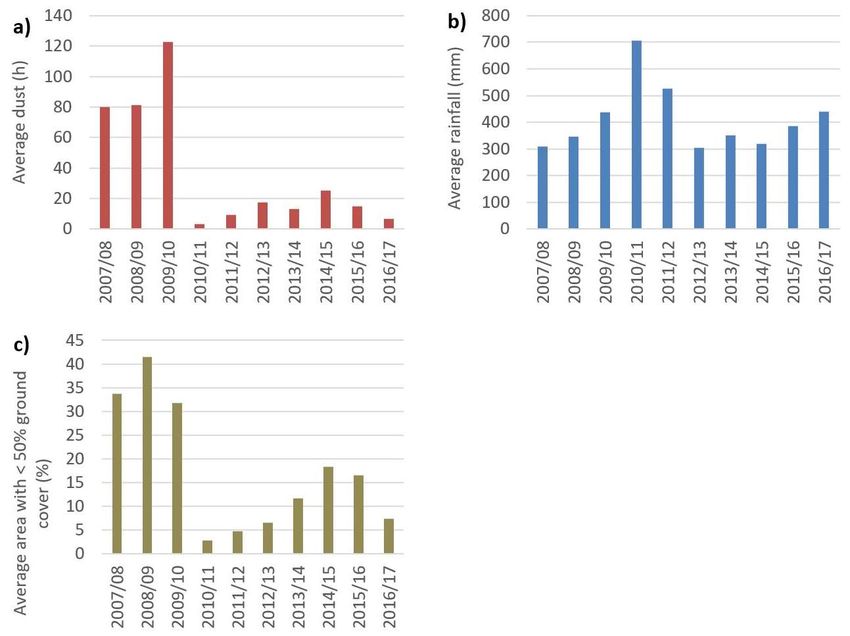
Geosciences 2018, 8, 232                                                                                 2 of 15

Environment in the U.S. [9] increase the awareness and heighten the need for monitoring programs [5,10].
However, land management practice change is a slow process. It took 13 years to increase the use of best
land management practices from 16 to 66% in the Mallee in Australia [11]. Measuring change therefore
requires long term monitoring that captures not only management change, but also the seasonal climate
variations [12]. Critical to all monitoring is that measurements are at the appropriate spatial and time scales.
      There are many examples of long term monitoring of dust activity from sediment and ice cores;
however, most core data are resolved at decadal or greater resolution. Sediment cores in China have
revealed a 1000 year history of dust activity in which authors conclude climate as the dominant driver [13].
Lake sediment core analyses from the San Juan Mountains of south-western Colorado, USA show increased
dust deposition following the arrival of western settlement and livestock grazing in the nineteenth and
the early twentieth century [14]. Ice-core samples from the Antarctic Peninsula showed dust deposition
doubled in the twentieth century due to increasing temperatures, decreasing relative humidity, and
widespread anthropogenic activity in Patagonia and northern Argentina [15]. Analysis of a 3200 year
marine core off West Africa at the century scale shows a marked increase in dust activity at the beginning
of the nineteenth century. This increase was linked to the advent of commercial agricultural activity in the
Sahel region [16]. While these very long term studies provide clear evidence of variable dust emissions,
and are even able to link increased dust with periods of land use change, the temporal scale is too coarse to
inform about land management practices and the spatial scale is limited.
      Global modelling of dust source areas and aerosol loads have also been used to identify spatial
patterns of wind erosion. A six year simulation (1990 to 1995) using 1.8◦ × 1.8◦ horizontal grid run on
six-hourly time steps found that the Sahara accounts for 58% of global dust emission and Australia
only 5.6% [17]. Whilst such studies provide ‘relative measure’ of global sources, the large grid sizes and
assumptions in the models, such as no soil disturbance, limit the modelling for monitoring. A single
year simulation (2000) using ~1.1◦ × 1.1◦ tested two soil input schema [18]. It found that increasing the
soil particle size distribution from three to four soil populations improved the model. The complexity
of these land/air models often results in multiple assumptions being tested and compromises being
made. For example, while soil population data may have improved, the fraction of ground cover for
each biome is estimated using a leaf area index and potential dust source regions, as defined by use
of the Olson’s global ecosystem biomes [19]. Using global ground cover and soils data at this scale
averages out heterogeneity within a grid cell.
      In recent years, there have been many studies using remote sensing to map and identify
dust source regions. Total Ozone Mapping Spectrometer (TOMS) has provided valuable global
measurements at daily temporal resolution with the trade-off of lower spatial resolution (50 by 50 km
at nadir). Use of TOMS data has identified global dust sources from multiyear studies [20–22], and
critically, linked dust sources with intermittently flooded regions [20,22], anthropogenic activity [20],
and climatic drivers [21]. In Australia, a 32 year record using TOMS linked dust emission to geomorphic
environments with pluvial activity [23]. This long record shows the importance of the Lake Eyre region
in central Australia, as reported by others [24]. However, like most remote sensing and modelling
studies, it fails to note the anthropogenic dust emission regions of the Mallee and other agricultural
areas in southern Australia. We believe this is consistent with areas in Kuwait, United States, and
the former Soviet Union where near surface dust is a common feature because dust storms are often
associated with cold fronts [25], which limit the dispersion of dust into the upper atmosphere [26].
      The Moderate Resolution Imaging Spectroradiometer (MODIS) has increased both spatial and
temporal resolution, producing images of 10 × 10 km twice a day. Using the cloud screened and quality
assured deep blue aerosol optical depth product derived from the Aqua platform of MODIS over a
seven year period (2003 to 2009), Ginoux et al. [27] differentiate global natural and anthropogenic dust
sources. Ginoux’s figure 5 shows a wider spatial distribution in eastern and northern Australia than
other remote sensing and modelling projects. However, it suffers similar issues to TOMS regarding
missing events with cloud cover.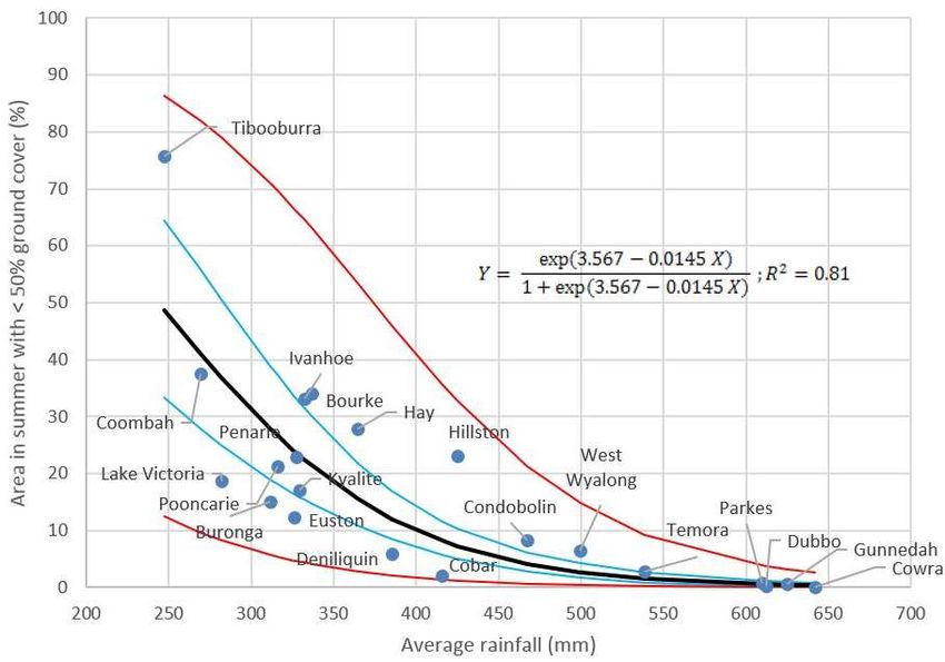
Geosciences 2018, 8, 232                                                                              3 of 15

     Most dust monitoring studies utilize meteorological records that record observed dust events.
Studies can be grouped as regional and global scales. Probably the longest regional record is that
for South Korea [28], which covers the time period 57BC to 2015. The later part of the record 1915 to
2015 was based on meteorological records. Lee, et al. [29] report the 42-year record (1947 to 1989)
for Lubbock, Texas. They report that wind and drought indexes are poor predictors of dust activity
due to the impact of agricultural land management practices. Middleton also under took several
studies in Australia [30], the Middle East [31], and south east Asia [32]. Using surface synoptic
observations (SYNOP) observations from 121 stations between 1960 to 2008, McTainsh et al. [33]
undertook Australia’s most detailed assessment of dust activity. For the meteorological data that they
used, they acknowledged how observational frequency, which ranges between one to eight times a
day, can bias results towards stations with high frequency of observations. This observational bias
is generally ignored in most studies. A longer time series using Australian meteorological records
was used to compare two periods (1937–1946 to 2001–2010) to investigate how dust levels changed
between the World War II drought and the Millennium Drought [34]. Global analysis has also been
undertaken by looking at specific regions over multiple decades of the world [35] and report how
drought and anthropogenic influences increase dust activity.
     Meteorological records, such as SYNOP and Meteorological Terminal Aviation Routine (METAR),
have been a fertile source of data. As O’Loingsigh, et al. [36] explain, the METAR offer better data
because they are taken more frequently (5–30 min intervals) and can be taken for a full 24 h as
airports have lights. Their study of the Millennium Drought (2000–2010) is probably one of the
highest quality studies using meteorological observations due to the duration and frequency of data;
however, the extent is limited to larger cities with airports. As Leys, et al. [37] point out, meteorological
observations are declining and so this data source is declining with time. Observers are being replaced
by instruments (e.g., nephelometers). Presently, in the drier western part of NSW, five nephelometer
stations exist, whereas 10 years ago, twice the number of observation sites existed.
     While advances in regional to global-scale remote sensing [27,38], field measurements [39,40], and
modelling techniques [18,41] have provided much improved data at moderate to high spatial scales,
they each have limitations. Remote sensing is not a continuous record and cloud cover is an issue.
Modelling, while improving all the time, still has large uncertainties that are caused by data scale and
availability. Field measurements also have limitations, such as cost and spatial coverage; however, in
the western New South Wales (NSW) region of south eastern Australia, we are fortunate to have set
up the DustWatch network of dust monitors a decade ago. These monitors collect data on one minute
time intervals 24 h a day. This overcomes the limitation of night time observations, cloud coverage,
and low frequency of observations.
     With this network, this study aims to answer commonly asked monitoring questions about wind
erosion in western NSW.

•     Where are the dusty places?
•     What are the trends in dust activity?
•     What thresholds of annual dust hours should we be striving to be below?

2. Materials and Methods
     This study utilizes two data sets, rainfall and total vegetation cover, to explain the variation in
dust data across western NSW.

2.1. Dust Data
      The 21 continuous dust monitoring sites (referred to as DustWatch Nodes—DWN, Figure 1) used in
this study form part of the Community DustWatch network [37] which in 2018 had 40 DWN (http://www.
environment.nsw.gov.au/topics/land-and-soil/soil-degradation/winderosion/community-dustwatch).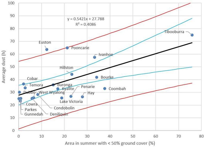
Figure 1) used in this study form part of the Community DustWatch network [37] which in 2018
      had 2018,
Geosciences 40 8,
                DWN
                  232  (http://www.environment.nsw.gov.au/topics/land-and-soil/soil-degradation/wind4 of 15
     erosion/community-dustwatch).

         Figure
     Figure     1. Location
            1. Location     of 21
                         of 21    DustWatchNodes
                               DustWatch    Nodes(DWN)
                                                  (DWN) with
                                                         with >10
                                                               >10years
                                                                   yearsofofrecords in in
                                                                              records  western NewNew
                                                                                          western  South
                                                                                                       South
         Wales (NSW) Australia, the 25 km radius sample circles used in study, and moderate-resolution
     Wales (NSW) Australia, the 25 km radius sample circles used in study, and moderate-resolution imaging
         imaging spectroradiometer (MODIS) Terra 24 October 2016 satellite image showing land cover.
     spectroradiometer (MODIS) Terra 24 October 2016 satellite image showing land cover.

     At each DWN, an 8520 model DustTrak® instrument measures the atmospheric aerosol
concentration of PM10, which is located inside the manufacture’s weatherproof environmental
enclosure. The DustTrak draws aerosols in a continuous stream through a non-heated sample inlet
and uses light scattering technology to determine mass concentration in real-time. The DustTrak is
programmed to sample every 15 min, increasing to one minute intervals when the PM10 concentration
exceeds 25 µg/m3 . Data is transferred to the Community DustWatch information interface (CoDii)
every 10 min where weighted hourly averages are calculated. If the hourly average concentration
exceeds 25 µg/m3 , then it is counted as one dust hour. We used 25 µg/m3 to signify a dust hour
because this equates to about a reduction of visibility to about 20 km [42]. From our experience with
volunteer DustWatchers, this is when they start to notice and report dust. We use the count of dust
hours as a measure of dust activity in this study.
     Quality control for each DustTrak is undertaken as follows:

•    Factory calibration is undertaken annually by the Australian distributor adjusted to respirable
     mass standard ISO 12103-1 Al Test Dust Arizona Dust. Calibration for a particular source material
     is not warranted as the network covers many sites across southern Australia with multiple dust
     source types.
•    Instruments are calibrated on site each month to have a zero (clean air) reading of ±3 µg/m3 .
     Inlets are cleaned and water bottles are emptied.
•    Every 15 min a zero reading is taken through the manufacturers ‘zero filter’ and stored in the
     database. This value is then subtracted from all of the ambient readings until the next zero filter
     reading is taken. This overcomes the problem of temperature variations or instrument drift.

     DustTraks measure all of the aerosols that are less than or equal to 10 µm aerodynamic diameter.
We subjectively classify the data in to fog, smoke, and dust. The standard operating method used to
classify DustWatch data is: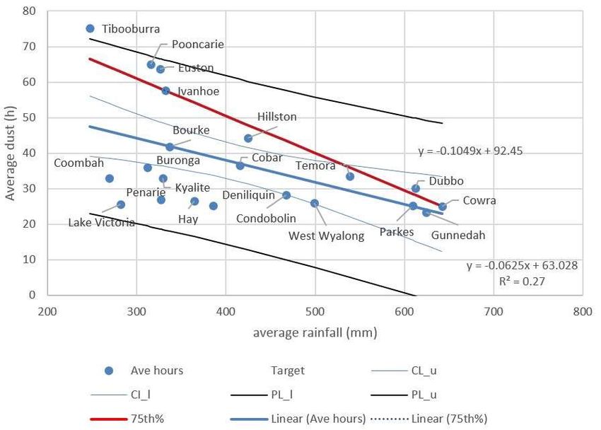
Geosciences 2018, 8, 232                                                                            5 of 15

•     All data are held within a purpose built supervisory control and data acquisition (SCADA)
      application called CoDii.
•     Each hourly reading is quality checked. CoDii downloads the data hourly and calculates the
      hourly time averaged aerosol concentration.
•     Values below 10 µg/m3 are not quality assessed because the DustWatch project is interested in
      higher concentrations for the detection of dust events.
•     Meteorological data from the nearest Australian Bureau of Meteorology automatic weather
      station and NASA MODIS Rapidfire data (http://lance-modis.eosdis.nasa.gov/imagery/subsets/
      ?project=other) are used to ascribe the hourly reading as dust, smoke, or fog using the
      following rules:

      1.     If values are above 10 µg/m3 —flag as dust unless following criteria are met. Note: While the
             manufacturer suggests instrument accuracy is about 3 µg/m3 , we choose to be conservative
             and do not use values less than 10 µg/m3 .
      2.     Flag as fog if:

             a.      humidity is high (>80%) and wind speed is low (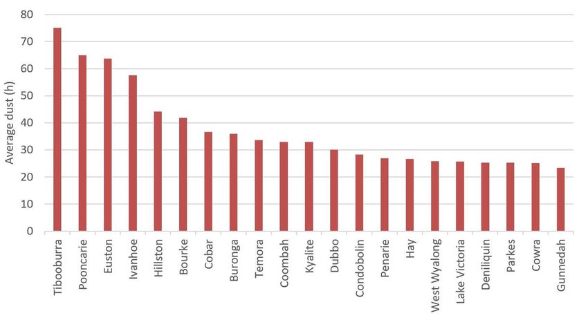
We use the CSIRO Land and Water algorithm for fractional cover derived from the moderate-
      resolution         imaging          spectroradiometer           (MODIS)         [43]       satellite      MODIS
      (http://data.auscover.org.au/xwiki/bin/view/Product+pages/Fractional+Cover+MODIS+CLW). The
      algorithm calculates the fraction of ground with in the 500 m pixel that is Photosynthetic Vegetation
      (PV), Non-Photosynthetic Vegetation (NPV), and Bare Soil (BS). We calculate the area within 25 km
      of each
Geosciences    DWN,
            2018, 8, 232which has a monthly total fraction of ground cover (PV+NPV) that is greater than 50%            6 of 15
      ground cover. The cut-off of 50% groundcover is used as this is the amount of ground cover required
      to control wind erosion [44]. The calculated values are stored in CoDii.
      In the study area of western NSW, ground cover changes with the seasons. Figure 2 shows the
            In the study area of western NSW, ground cover changes with the seasons. Figure 2 shows the
monthly     average
      monthly           of the
                  average       2121
                            of the sites
                                      sitesfor
                                             forthe
                                                  the2525km
                                                          km area   aroundall
                                                              area around   allthe
                                                                                 theDWN
                                                                                     DWN      during
                                                                                           during  thisthis
                                                                                                        ten ten
                                                                                                            yearyear
                                                                                                                 study.study.
The area     withwith
      The area
Geosciences 2018, 8, 232 7 of 15
3.2. Trends
The number of hours of dust, rainfall, and area with groundcover < 50% within 25 km of each
DWN changes from year to year (Figure 4). The first three years from 2007/08 to 2009/10 were during
the end of the Millennial Drought. During this dry time, the area of ground cover < 50% and dust
hours where the highest. Very high rainfall was recorded in 2010/11, and the area of ground cover <
Geosciences
50% and 2018,
dust8,levels
x FOR dropped
PEER REVIEW
dramatically. 8 of 16
Figure
Figure 4.
4. (a) Averagedust
(a) Average dusthours
hoursfor
forthe
the2121DustWatch
DustWatch Nodes
Nodes (DWN),
(DWN), (b)(b) average
average rainfall
rainfall within
within 25
25 km,
km,
and and (c) average
(c) average areaarea
withwith less than
less than 50% 50% ground
ground covercover for each
for each DustDust
StormStorm
Year Year (DSY).
(DSY).
3.3. Dust Targets
3.3. Dust Targets
Each DWN has a different range of observed dust hours. But, what is the ‘normal’ level of dust
Each DWN has a different range of observed dust hours. But, what is the ‘normal’ level of dust
hours for NSW across the 98 to 967 mm rainfall gradient? As McTainsh and Leys [45] and many other
hours for NSW across the 98 to 967 mm rainfall gradient? As McTainsh and Leys [45] and many other
authors have shown, the level of dust activity increases with a decrease in rainfall. In this paper, we
authors have shown, the level of dust activity increases with a decrease in rainfall. In this paper, we
define a dust ‘target’ as ‘a level that is better than what is currently being achieved’. To determine
define a dust ‘target’ as ‘a level that is better than what is currently being achieved’. To determine what
what the target dust hours should be across the rainfall gradient, we used quantile regression
the target dust hours should be across the rainfall gradient, we used quantile regression methods [46]
methods [46] (Figure 5). The concept is that, ideally, a DWN with a given DSY rainfall should have
(Figure 5). The concept is that, ideally, a DWN with a given DSY rainfall should have less dust hours
less dust hours than the 75th percentile of the benchmark decade between 2007/08 and 2016/17 (red
than the 75th percentile of the benchmark decade between 2007/08 and 2016/17 (red line in Figure 5).
line in Figure 5). The results for the 75th percentile regression results in Equation (1):
The results for the 75th percentile regression results in Equation (1):
DT = −0.10 × DSY + 92.45, (1)
DT = −0.10 × DSY + 92.45, (1)
where DY = dust target (h) and DSY = average DSY rainfall (mm). This closely approximates a 10 h
reduction
where DYin DSY dust
= dust targethours for DSY
(h) and each =100 mm increase
average in DSY
DSY rainfall rainfall,
(mm). Thisbetween
closely 250 and 650 mm.
approximates a 10 h
reduction in DSY dust hours for each 100 mm increase in DSY rainfall, between 250 and 650 mm. for
The number of dust hours measured at each DWN for each DSY and the target dust hours
each The
DWN based on
number Equation
of dust hours(1)measured
are givenatineach
Table 1. for each DSY and the target dust hours for
DWN
each DWN based on Equation (1) are given in Table 1.Geosciences 2018, 8, 232 8 of 15
Geosciences 2018, 8, x FOR PEER REVIEW 9 of 16
Figure 5.
Figure 5. Relationship
Relationshipbetween average
between DSYDSY
average rainfall and average
rainfall dust hours
and average dust for 21 DWN.
hours for 21Standard
DWN.
regression (Linear Ave hours—thick blue line), 90% confidence (CL_u and CL_l—thin blue
Standard regression (Linear Ave hours—thick blue line), 90% confidence (CL_u and CL_l—thin blue lines) and
prediction
lines) (PL_u and(PL_u
and prediction PL_L—thin black lines)
and PL_L—thin limits.
black Target
lines) dust
limits. hoursdust
Target represented by 75th percentile
hours represented by 75th
regressionregression
percentile line (75th%)—thick red line. red line.
line (75th%)—thickGeosciences 2018, 8, 232 9 of 15
Table 1. Hours of dust for each DustWatch Node (DWN) for each DSY, average hours and the target number of dust hours (h) from Equation 1.
DWN 2007/08 2008/09 2009/10 2010/11 2011/12 2012/13 2013/14 2014/15 2015/16 2016/17 Average Target
Bourke 86 49 201 2 22 13 23 19 0 4 42 57
Buronga 54 74 113 7 30 25 14 33 9 1 36 60
Cobar 85 77 128 5 13 16 12 23 1 6 37 49
Condobolin 95 77 50 3 4 9 16 19 9 1 28 43
Coombah 45 49 155 1 0 20 26 17 16 1 33 64
Cowra 44 43 135 0 1 5 1 14 1 7 25 25
Deniliquin 57 61 36 2 14 20 13 28 16 6 25 52
Dubbo 34 62 110 2 2 12 32 34 5 8 30 28
Euston 85 135 141 2 15 107 12 61 63 16 64 58
Gunnedah 52 19 113 1 0 5 17 12 14 1 23 27
Hay 47 84 61 1 1 10 16 29 11 6 27 54
Hillston 98 138 113 4 14 12 11 33 8 11 44 48
Ivanhoe 131 168 216 3 11 5 3 15 17 7 58 58
Kyalite 65 75 43 2 15 25 13 29 44 18 33 58
Lake Victoria 43 35 108 5 10 11 3 9 29 4 26 63
Parkes 77 46 95 2 2 10 0 15 3 3 25 29
Penarie 63 67 35 2 9 23 16 20 30 5 27 58
Pooncarie 210 195 143 6 3 12 18 39 10 14 65 59
Temora 113 82 85 10 4 2 4 22 8 6 34 36
Tibooburra 116 121 413 0 16 6 23 37 15 4 75 66
West Wyalong 75 47 82 3 4 18 4 18 3 5 26 40Geosciences 2018, 8, 232 10 of 15
4. Discussion
The results of this study cover a wide range of dust, rainfall, and ground cover levels. This is
because the ten year study period covered one of the driest [47] and wettest periods [48] in
south-eastern Australia. Having a data set that covers such climate extremes is fortunate, as it gives us
confidence we have measurements of extremes of dust (0 to 412 h/DSY), rainfall (98 to 967 mm/DSY),
and ground cover (0 to 99% of area/DSY). While it is possible to derive individual rainfall/dust hour
relationships for each DWN, the aim here was to look at dust activity across western NSW; thus, we
use a regression model based on all sites and set a target that is based on the ensemble of all sites.
Our results support the findings of McTainsh and Leys [45] that rainfall is a driver of dust
activity; however, the relationship in Figure 5 is not strong (R2 = 0.27). This is not surprising as
there are many other factors that influence wind erosion. These include soil erodibility, if a site has
perennial or annual vegetation, and anthropogenic activities, like farming. Sandy soils have higher
erodibility [49,50] and cropping areas often have bare soil prior to planting crops (fallow phase) that
have high erodibility [44,50]. Sites that are close to fluvial basins are often highly erodible [51,52].
In Figure 5, there are several DWN that sit outside the 90% confidence intervals (CI). For example,
Coombah and Lake Victoria have permanent native vegetation with trees around them, Euston and
Pooncarie are in farming areas with sandy soils, and Tibooburra is located down wind of Australia’s
largest dust source, the Lake Eyre Basin [12,52,53]. All of these factors add to the spread in the data.
The trends show the influence of the changing rainfall over the period (Figure 4). That is, when
dust activity was high in the beginning of the study period (Figure 4a) when rainfall (Figure 4b) was
comparatively low and the corresponding area with ground cover < 50% was high (Figure 4c). With the
high rainfall in 2010/11 and 2011/12 the area with low ground cover ground cover area decreased and
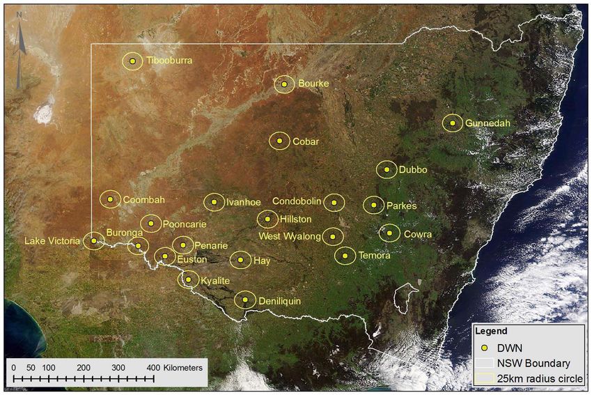
so do the dust hours. The curvilinear relationship between rainfall and percentage area < 50% ground
cover in summer is shown in Figure 6. We have used a logit transformation of the response variable
because of the sigmoidal shape of the relationship with rainfall, but equally importantly to ensure
that the fitted values and derived confidence and prediction limits remain within the sensible bounds
of 0% and 100% area withGeosciences 2018, 8, 232 11 of 15
Geosciences 2018, 8, x FOR PEER REVIEW 12 of 16
Geosciences 2018, 8, x FOR PEER REVIEW 12 of 16
Figure 6. Relationship between average DSY rainfall and percentage area < 50% ground cover (in
Figure 6. Relationship between average DSY rainfall and percentage area < 50% ground cover
Figure 6.months
summer Relationship between
of DJF). average
Standard DSY rainfall
regression and percentage
(Curvilinear area < 50% black
GCA < 50%—thick groundline),
cover (in
90%
(in summer months of DJF). Standard regression (Curvilinear GCA < 50%—thick black line), 90%
summer months
confidence of DJF).
(CL_u and Standard
CL_l—thin blueregression (Curvilinear
lines) and prediction GCA
(PL_u < PL_L—thin
and 50%—thick red
black line),
lines) 90%
limits.
confidence (CL_u and CL_l—thin blue lines) and prediction (PL_u and PL_L—thin red lines) limits.
confidence (CL_u and CL_l—thin blue lines) and prediction (PL_u and PL_L—thin red lines) limits.
Figure 7. Relationship between percentage area < 50% in summer months and dust hours. Standard
Figure 7. Relationship
regression (Linear Ave between percentage
hours—thick areaGeosciences 2018, 8, 232 12 of 15
Partitioning dust emissions from either natural or anthropogenic sources is extremely difficult
in a region of mixed land uses, such as south eastern Australia. Climate drives large geomorphic
dust sources, such as the Lake Eyre floodplains [38,53], along with incremental changes in ground
cover associated with season or drought [29,33–35]. Whilst remote sensing techniques, such as TOMS
and MODIS, can provide valuable data regarding aerosol loading [20,27] and even locate small
dust source areas [38], they cannot reliably inform us about the anthropogenic nature of the dust,
particularly in the rangelands. Frequently, land use maps are used as determinants of natural or
anthropogenically modified surfaces in modelling and remote sensing studies. Prospero et al. [20]
argue the Tegan and Fung [54] estimate of 20–50% of global dust emissions that are associated with land
use as being overly high given that the largest dust sources are associated with very low populations.
However, rangelands are managed for grazing and thus have anthropogenic influences. Using MODIS
Deep Blue, Ginoux et al. [27] estimate anthropogenic dust to be 25% due to land use. This study shows
that the low population areas, like Tibooburra (90 people within 25 km—2011 census) and Ivanhoe
(231 people within 25 km—2011 census), have high dust activity and low population. We believe there
is a strong anthropogenic contribution to dust emission in rangelands of eastern Australia.
The DustWatch network across NSW has provided an alternative approach to identify regions
that record higher hours of dust than expected. By setting yearly dust hour targets for NSW based on
the DSY rainfall we see an average 10 h drop in the dust target hours for every 100 mm increase in
DSY rainfall between 250 and 650 mm.
These targets are a guide as to what dust activity might be achieved across the rainfall gradient
of western NSW. Whilst the overall trend in dust activity over the decade was one of decline, there
are two stations that have reversed the strong influence of rainfall, suggesting that land management
is driving the dust emission (Table 1). Euston DWN is a farming area on high erodible sandy soils
and is also down-wind of the dryland farming areas of north-west Victoria, which are infamous for
its wind erosion [2]. The largest exceedance for Euston was in 2012/13, and was due to poor crop
growth in the 2012 growing season that resulted in very low ground cover in the region. The following
quote from the February 2013, DustWatch report [55], outlines the cause of the dust. “Although the
majority of paddocks in the northern Mallee have the previous season’s stubble present, there is low
groundcover remaining, due to low 2012 growing season rainfall; low 2012/13 summer rainfall; and
summer grazing pressure. The stubble is very thin through-out most paddocks and the wind has
started to blow some of the higher areas”. Dubbo is the other DWN that had exceedances in 2013/14,
and 2014/15. There was wide spread dust activity in January and February 2014 to the north of Dubbo,
and in November 2014, Walgett had 139 h of dust [56–58]. It is probable that dust has blown south to
Dubbo. This long-range transport of dust indicates one of the limitations of this analysis; that is, dust
at one DWN may not be local. However, these targets are based on the 21 DWN and are based on the
sample population, representing western NSW, and not a specific site. Therefore, we can now assess
the level of dust in future years against the benchmark 75% percentile dust targets. The aim being to
not exceed the target for a given DSY rainfall. If the targets are exceeded, then investigation should
occur to see why there is excessive dust.
5. Conclusions
This paper posed the following three questions, and the answers are:
• Where are the dusty places? Not surprisingly, Tibooburra is the dustiest place in NSW. This is a
function of its low rainfall and location down-wind of the Lake Eyre Basin. The data also indicates
that semi-arid dryland farming areas, like Euston and Pooncarie, are dusty. Once again, not
surprising considering the low rainfall and the risks of semi-arid dryland farming.
• What are the trends in dust activity? The trend over the last decade in NSW has been downwards;
however, this is a function of rainfall. Within the rainfall dust relationship, are other factors,
like land use (farming), erodibility of the landscape (sandy soil areas have higher erosion), and
perenniality of the vegetation (treed areas tend to have less dust).Geosciences 2018, 8, 232 13 of 15
• What levels of dust should we be aiming for? This data set has enabled us to set DSY dust hour
targets for NSW based on the DSY rainfall. Basically, there is a 10 h drop in the dust target for
every 100 mm increase in DSY rainfall between 250 and 650 mm. These targets are guides as to
what dust activity might be expected across western NSW. They can be used to investigate the
performance of the land management systems and to report the state of the environment of NSW.
Future research aims to set dust targets for each DWN. With over forty DWN in the Community
DustWatch network, this will provide an excellent way of reporting against Government environmental
programs, such as the State of the Environment. Also, the approach that is used in Figure 7 could be
used to set ground cover targets for individual DWN.
Author Contributions: The lead author, J.L. leads the DustWatch project and as such conceptualized and prepared
the original draft, including preliminary analysis. C.S. contributed to data, writing, reviewing and editing. T.K. was
responsible for statistical analyses. S.H. developed the equipment and databases used in this study. He also
manages CoDii, assisted with data analysis and preparation of figures.
Funding: The DustWatch project has received funding over the 10 year study period from Office of Environment
and Heritage, the Department of Agriculture and Water Resources, National Landcare Program, Western, Riverina,
Murray, Central Tablelands, and Central West Local Land Services.
Acknowledgments: Dust data supplied by the Office of Environment and Heritage Rural Air Quality network.
The MODIS image is courtesy of MODIS Rapid Response Project at NASA/GSFC; rainfall data from the
Australian Bureau of Meteorology. Ground cover data supplied by Commonwealth Scientific Industrial Research
Organisation. We particularly thank our many DustWatch volunteers who provide observations and help maintain
the instruments and Joanne Brady for quality assurance of the DustWatch data.
Conflicts of Interest: The authors declare no conflict of interest.
References
1. Middleton, N.J.; Goudie, A.S. Saharah dust: Sources and trajectories. Trans. Inst. Br. Geogr. 2001, 26, 165–181.
[CrossRef]
2. Cattle, S.R. The case for a southeastern Australian Dust Bowl, 1895–1945. Aeolian Res. 2016, 21, 1–20.
[CrossRef]
3. Leys, J.; Smith, J.; MacRae, C.; Rickards, J.; Yang, X.; Randall, L.; Hairsine, P.; Dixon, J.; McTainsh, G.
Improving the Capacity to Monitor Wind and Water Erosion: A Review; Department of Agriculture, Fisheries and
Forests, Australian Government: Canberra, Australia, 2009; p. 160.
4. Webb, N.P.; Van Zee, J.W.; Karl, J.W.; Herrick, J.E.; Courtright, E.M.; Billings, B.J.; Boyd, R.; Chappell, A.;
Duniway, M.C.; Derner, J.D.; et al. Enhancing Wind Erosion Monitoring and Assessment for U.S. Rangelands.
Rangelands 2017, 39, 85–96. [CrossRef]
5. Australian Government. National Landcare Programme. Available online: http://www.nrm.gov.au/
national-landcare-programme (accessed on 30 August 2017).
6. Australian Government Department of Environment and Heritage. Australia State of the Environment 2006: At
a Glance; Australian Government Department of Environment and Heritage: Canberra, Australia, 2006; p. 16.
7. Metcalfe, D.J.; Bui, E.N. Australia State of the Environment 2016: Land, Independent Report to the Australian
Government Minister for the Environment and Energy; Australian Government Department of the Environment
and Energy: Canberra, Australia, 2017.
8. European Environment Agency. The European Environment—State and Outlook: Synthesis Report; European
Environment Agency: Copenhagen, Denmark, 2015; p. 205.
9. United States Environmental Protection Agency. Report on the Environment; National Center for
Environmental Assessment: Washington, DC, USA, 2008; p. 366.
10. Webb, N.P.; Herrick, J.E.; Van Zee, J.W.; Courtright, E.M.; Hugenholtz, C.H.; Zobeck, T.M.; Okin, G.S.;
Barchyn, T.E.; Billings, B.J.; Boyd, R.; et al. The National Wind Erosion Research Network: Building a
standardized long-term data resource for aeolian research, modeling and land management. Aeolian Res.
2016, 22, 23–36. [CrossRef]
11. Leys, J.; Heidenreich, S.; Koen, T.; Colson, I. DustWatch Network and Roadside Survey 2016; Report for Contract
WN00732; NSW Government, Local Land Services: Dubbo, Australia, 2016; p. 27.Geosciences 2018, 8, 232 14 of 15
12. Strong, C.L.; Parsons, K.; McTainsh, G.H.; Sheehan, A. Dust transporting wind systems in the lower Lake
Eyre Basin, Australia: A preliminary study. Aeolian Res. 2011, 2, 205–214. [CrossRef]
13. He, Y.; Zhao, C.; Song, M.; Liu, W.; Chen, F.; Zhang, D.; Liu, Z. Onset of frequent dust storms in northern
China at ~AD 1100. Sci. Rep. 2015, 5, 17111. [CrossRef] [PubMed]
14. Toney, J.L.; Anderson, R.S. A postglacial palaeoecological record from the San Juan Mountains of Colorado
USA. Holocene 2006, 16, 505–517. [CrossRef]
15. McConnell, J.R.; Aristarain, A.J.; Banta, J.R.; Edwards, P.R.; Simões, J.C. 20th-Century doubling in dust
archived in an Antarctic Peninsula ice core parallels climate change and desertification in South America.
Proc. Natl. Acad. Sci. USA 2007, 104, 5743–5748. [CrossRef] [PubMed]
16. Mulitza, S.; Heslop, D.; Pittauerova, D.; Fischer, H.W.; Meyer, I.; Stuut, J.-B.; Zabel, M.; Mollenhauer, G.;
Collins, J.A.; Kuhnert, H.; et al. Increase in African dust flux at the onset of commercial agriculture in the
Sahel region. Nature 2010, 166, 226–228. [CrossRef] [PubMed]
17. Tanaka, T.Y.; Chiba, M. A numerical study of the contributions of dust source regions to the global dust
budget. Glob. Planet. Chang. 2006, 52, 88–104. [CrossRef]
18. Astitha, M.; Lelieveld, J.; Abdel Kader, M.; Pozzer, A.; de Meij, A. Parameterization of dust emissions in the
global atmospheric chemistry-climate model EMAC: Impact of nudging and soil properties. Atmos. Chem. Phys.
2012, 12, 11057–11083. [CrossRef]
19. Olson, J.S. World Ecosystems (WE1.4). Digital Raster Data on a 10-Minute Cartesian Orthonormal Geodetic
1080 × 2160 Grid. Available online: http://ref.data.fao.org/map?entryId=be34dd90-88fd-11da-a88f-
000d939bc5d8&tab=about (accessed on 6 May 2018).
20. Prospero, J.M.; Ginoux, P.; Torres, O.; Nicholsan, S.E.; Gill, T. Environmental characterisation of global
sources of atmospheric soil dust identified with the NIMBUS-7 total ozone mapping spectrometer (TOMS)
absorbing aerosol product. Rev. Geophys. 2002, 40, 2-1–2-31. [CrossRef]
21. Washington, R.; Todd, M.; Middleton, N.J.; Goudie, A.S. Dust-storm source areas determined by the Total
Ozone Monitoring Spectrometer and surface observations. Ann. Assoc. Am. Geogr. 2003, 93, 297–313.
[CrossRef]
22. Varga, G. Spatio-temporal distribution of dust storms—A global coverage using NASA TOMS aerosol
measurements. Hung. Geogr. Bull. 2012, 61, 275–298.
23. Baddock, M.; Bullard, J.; McTainsh, G.H.; Leys, J.F. Linking Geomorphology and Dust Emission: Identifying Dust
Sources at the Sub-Basin Scale, Lake Eyre Basin Australia; British Geomorphological Research Group (BGRG)
Workshop, “Another Windy Day at Northampton”, University of Northampton; British Geomorphological
Research Group, University of Northampton: Northampton, UK, 2007.
24. Baddock, M.C.; Bullard, J.E.; Bryant, R.G. Dust source identification using MODIS: A comparison of
techniques applied to the Lake Eyre Basin, Australia. Remote Sens. Environ. 2009, 113, 1511–1528. [CrossRef]
25. Raupach, M.R.; McTainsh, G.H.; Leys, J.F. Estimates of dust mass in recent major dust storms. Aust. J. Soil
Water Conserv. 1994, 7, 20–24.
26. McGowan, H.; Clark, A. A vertical profile of PM10 dust concentrations measured during a regional dust
event identified by MODIS Terra, western Queensland, Australia. J. Geophys. Res. 2008, 113. [CrossRef]
27. Ginoux, P.; Prospero, J.M.; Gill, T.E.; Hsu, N.C.; Zhao, M. Global-scale attribution of anthropogenic and
natural dust sources and their emission rates based on MODIS Deep Blue aerosol products. Rev. Geophys.
2012, 50. [CrossRef]
28. Chun, Y.; Cho, H.; Chung, H.; Lee, M. From Historical Records to Early Warning System of Asian dust
(Hwangsa) in Korea. Bull. Am. Meteorol. Soc. 2008, 86, 823–827. [CrossRef]
29. Lee, J.A.; Wigner, K.A.; Gregory, J.M. Drought, Wind and Blowing Dust on the Southern High Plains of the
United States. Phys. Geogr. 1993, 14, 56–67.
30. Middleton, N.J. Dust storms in Australia: Frequency, distribution and seasonality. Search 1984, 15, 46–47.
31. Middleton, N.J. Dust storms in the Middle East. J. Arid Environ. 1984, 10, 83–96.
32. Middleton, N.J. A geography of dust storms in South-West Asia. J. Climatol. 1986, 6, 183–196. [CrossRef]
33. McTainsh, G.; Strong, C.; Leys, J.; Baker, M.; Tews, K.; Barton, K. Wind Erosion Histories, Model Input Data and
Community DustWatch; Atmospheric Environment Research Centre, Griffith University: Brisbane, Australia,
2009; p. 221.Geosciences 2018, 8, 232 15 of 15
34. O’Loingsigh, T.; McTainsh, G.H.; Parsons, K.; Strong, C.L.; Shinkfield, P.; Tapper, N.J. Using meteorological
observer data to compare wind erosion during two great droughts in eastern Australia; the World War II
Drought (1937–1946) and the Millennium Drought (2001–2010). Earth Surf. Process. Landf. 2015, 40, 123–130.
[CrossRef]
35. Goudie, A.S.; Middleton, N.J. The changing frequency of dust storms through time. Clim. Chang. 1992, 20,
197–225. [CrossRef]
36. O’Loingsigh, T.; Chubb, T.; Baddock, M.; Kelly, T.; Tapper, N.J.; De Deckker, P.; McTainsh, G. Sources and
pathways of dust during the Australian “Millennium Drought” decade. J. Geophys. Res. 2017, 122, 1246–1260.
[CrossRef]
37. Leys, J.F.; McTainsh, G.H.; Strong, C.L.; Heidenreich, S.; Biesaga, K. DustWatch: Using community networks
to improve wind erosion monitoring in Australia. Earth Surf. Process. Landf. 2008, 33, 1912–1926. [CrossRef]
38. Bullard, J.; Baddock, M.; McTainsh, G.; Leys, J. Sub-basin scale dust source geomorphology detected using
MODIS. Geophys. Res. Lett. 2008, 35, L15404. [CrossRef]
39. Nickling, W.G.; McTainsh, G.H.; Leys, J.F. Dust emissions from the Channel Country of western Queensland,
Australia. Z. Geomorphol. Suppl. 1999, 116, 1–17.
40. Sharratt, B.; Wendling, L.; Feng, G. Surface characteristics of a windblown soil altered by tillage intensity
during summer fallow. Aeolian Res. 2012, 5, 1–7. [CrossRef]
41. Alfaro, S.C.; Gomes, L. Modelling mineral aerosol production by wind erosion: Emission intensities and
aerosol size distributions in source areas. J. Geophys. Res. 2001, 106, 18075–18084. [CrossRef]
42. Baddock, M.C.; Strong, C.L.; Leys, J.F.; Heidenreich, S.K.; Tews, E.K.; McTainsh, G.H. A visibility and total
suspended dust relationship. Atmos. Environ. 2014, 89, 329–336. [CrossRef]
43. Guerschman, J.P.; Scarth, P.F.; McVicar, T.R.; Renzullo, L.J.; Malthus, T.J.; Stewart, J.B.; Rickards, J.E.;
Trevithick, R. Assessing the effects of site heterogeneity and soil properties when unmixing photosynthetic
vegetation, non-photosynthetic vegetation and bare soil fractions from Landsat and MODIS data.
Remote Sens. Environ. 2015, 161, 12–26. [CrossRef]
44. Leys, J.F. Wind erosion on agricultural land. In Aeolian Environments, Sediments and Landforms; Goudie, A.S.,
Livingston, I., Stokes, S., Eds.; John Wiley and Sons: Chinchester, UK, 1999; pp. 143–166.
45. McTainsh, G.H.; Leys, J.F. Soil Erosion by Wind; Longman Cheshire: Melbourne, Australia, 1993; pp. 188–233.
46. Koenker, R.; Hallock, K. Quantile regression: An introduction. J. Econ. Perspect. 2001, 15, 143–156. [CrossRef]
47. Bureau of Meteorology. Annual Climate Summary. 2009. Available online: http://www.bom.gov.au/
climate/annual_sum/2009/AnClimSum09_LR1.1.pdf (accessed on 22 April 2018).
48. Bureau of Meteorology. Annual Climate Summary. 2010. Available online: http://www.bom.gov.au/
climate/annual_sum/2010/AnClimSum10_HR1.0.pdf (accessed on 22 April 2018).
49. Leys, J.F. The threshold friction velocities and soil flux rates of selected soils in south-west New South Wales,
Australia. Acta Mech. 1991, 2, 103–112.
50. Chepil, W.S. Factors that influence clod structure and erodibility by wind. I. Soil texture. Soil Sci. 1953, 75,
473–483. [CrossRef]
51. McTainsh, G. Harmattan dust deposition in Northern Nigeria. Nature 1980, 286, 587–588. [CrossRef]
52. Bullard, J.E.; McTainsh, G.H. Aeolian-fluvial interactions in dryland environments: Examples, concepts and
Australian case study. Prog. Phys. Geogr. 2003, 27, 471–501. [CrossRef]
53. Baddock, M.C.; Parsons, K.; Strong, C.L.; Leys, J.F.; McTainsh, G.H. Drivers of Australian dust: A case
study of frontal winds and dust dynamics in the lower Lake Eyre Basin. Earth Surf. Process. Landf. 2015, 40,
1982–1988. [CrossRef]
54. Tegen, I.; Fung, I. Contribution to the atmospheric mineral aerosol load from land surface modification.
J. Geophys. Res. 1995, 100, 18707–18726. [CrossRef]
55. DustWatch. DustWatch Report February 2013; Office of Environment and Heritage: Sydney, Australia, 2013; p. 4.
56. DustWatch. DustWatch Report February 2014; Office of Environment and Heritage: Sydney, Australia, 2014; p. 4.
57. DustWatch. DustWatch Report January 2014; Office of Environment and Heritage: Sydney, Australia, 2014; p. 3.
58. DustWatch. DustWatch Report November 2014; Office of Environment and Heritage: Sydney, Australia, 2014; p. 6.
© 2018 by the authors. Licensee MDPI, Basel, Switzerland. This article is an open access
article distributed under the terms and conditions of the Creative Commons Attribution
(CC BY) license (http://creativecommons.org/licenses/by/4.0/).You can also read