Why Did So Many Subprime Borrowers Default During the Crisis: Loose Credit or Plummeting Prices?
←
→
Page content transcription
If your browser does not render page correctly, please read the page content below
Why Did So Many Subprime Borrowers Default During the Crisis:
                           Loose Credit or Plummeting Prices?∗

                                              Christopher Palmer†
                                                        MIT

                                              November 15, 2013

                                          JOB MARKET PAPER

                                                     Abstract

          The foreclosure rate of subprime mortgages increased markedly across 2003–2007
      borrower cohorts—subprime mortgages originated in 2006–2007 were roughly three
      times more likely to default within three years of origination than mortgages origi-
      nated in 2003–2004. Many have argued that this surge in subprime defaults represents
      a deterioration in subprime lending standards over time. I quantify the importance of
      an alternative hypothesis: later cohorts defaulted at higher rates in large part because
      house price declines left them more likely to have negative equity. Using loan-level
      data, I find that changing borrower and loan characteristics explain approximately 30%
      of the difference in cohort default rates, with almost of all of the remaining heterogeneity
      across cohorts attributable to the price cycle. To account for the endogeneity of prices,
      I employ a nonlinear instrumental-variables approach that instruments for house price
      changes with long-run regional variation in house-price cyclicality. Control function
      results confirm that the relationship between price declines and defaults is causal and
      explains the majority of the disparity in cohort performance. I conclude that if 2006
      borrowers had faced the same prices the average 2003 borrower did, their annual default
      rate would have dropped from 12% to 5.6%.

      Keywords: Mortgage Finance, Subprime Lending, Foreclosure Crisis, Negative Equity
      JEL Classification: G01, G21, R31, R38
   ∗
     For the latest version of my job market paper, see http://mit.edu/cjpalmer/www/CPalmer JMP.pdf. I thank
my advisors, David Autor, Jerry Hausman, Parag Pathak, and Bill Wheaton, for their feedback and encouragement;
Isaiah Andrews, John Arditi, Matthew Baird, Stan Carmack, Marco Di Maggio, Dan Fetter, Chris Foote, Chris
Gillespie, Wills Hickman, Amir Kermani, Lauren Lambie-Hanson, Brad Larsen, Eric Lewis, Whitney Newey, Brian
Palmer, Jonathan Parker, Bryan Perry, Brendan Price, Adam Sacarny, Dan Sullivan, Glenn Sueyoshi, Chris Walters,
Nils Wernerfelt, Paul Willen, Heidi Williams, and Tyler Williams for helpful discussions and feedback; participants at
the MIT Applied Microeconomics, Econometrics, and Public Finance workshops; and seminar participants at MIT.
The loan-level data used herein was provided by CoreLogic.
   †
     PhD Candidate, MIT Economics; cjpalmer@mit.edu
1     Introduction

Subprime residential mortgage loans were ground zero in the Great Recession, comprising over 50%
of all 2006–2008 foreclosures despite the fact that only 13% of existing residential mortgages were
subprime at the time.1 The subprime default rate—the number of new subprime foreclosure starts
as a fraction of outstanding subprime mortgages—tripled from under 6% in 2005 to 17% in 2009.
By 2013, more than one in five subprime loans originated since 1995 had defaulted. While subprime
borrowers by definition have been ex-ante judged as having greater default risk than non-subprime
mortgages, many have pointed to the disproportionate growth in the share of defaults by subprime
borrowers as evidence that the expansion in subprime lending was a major contributing cause to
the housing crash of 2007–2009.
    Why did the performance of subprime loans decline so sharply? A focal point of the discussion
has been the stylized fact that subprime mortgages originated in 2005–2007 performed significantly
worse than subprime mortgages originated in 2003–2004.2 This is visible in the top panel of Figure
1, which uses data from subprime private-label mortgage-backed securities to show this pattern for
2003–2007 borrower cohorts.3 Each line shows the fraction of borrowers in the indicated cohort
that defaulted within a given number of months from origination.4 The pronounced pattern is
that the speed and frequency of default are higher for later cohorts—within any number of months
since origination, more recent cohorts have defaulted at a higher rate (with the exception of the
2007 cohort in later years). For example, within two years of origination, approximately 20% of
subprime mortgages originated in 2006–2007 had defaulted, in contrast with approximately 5% of
2003-vintage mortgages.
    A popular explanation for the heterogeneity in cohort-level default rates over time is that loosen-
    1
      Statistics derived from the Mortgage Bankers Association National Delinquency Survey. There is no standardized
definition of a subprime mortgage, although the term always means a loan deemed to have elevated default risk.
Popular classification methods include mortgages originated to borrowers with a credit score below certain thresholds,
mortgages with an interest rate that exceeds the comparable Treasury Bill rate by 3%, certain mortgage product
types, mortgages made by lenders who self-identify as making predominantly subprime mortgages, and mortgages
serviced by firms that specialize in servicing subprime mortgages. For the purposes of this paper, subprime mortgages
are defined as those in private-label mortgage-backed securities marketed as subprime, as in Mayer et al. (2009). For
an estimate of the effects of foreclosures on the real economy, see Mian et al. (2011).
    2
      See JEC (2007), Krugman (2007b), Gerardi et al. (2008), Haughwout et al. (2008), Mayer et al. (2009), Demyanyk
and Van Hemert (2010), and Bhardwaj and Sengupta (2011) for examples of contrasting earlier and later borrower
cohorts.
    3
      This data will be discussed at length in Section 3. The analysis stops in 2007 because by 2008 the subprime
securitized market was virtually nonexistent—the number of subprime loans originated in 2008 in the data fell by
99% from the number of 2007 originations.
    4
      Following Sherlund (2008) and Mayer et al. (2009), I measure the point in time when a mortgage has defaulted
as the first time that its delinquency status is marked as in foreclosure or real-estate owned provided it ultimately
terminated without being paid off in full.

                                                          1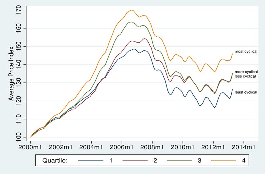
ing lending standards led to a change in the composition of subprime borrowers, potentially on both
observable and unobservable dimensions (e.g. JEC, 2007 and COP, 2009). Others (e.g. Krugman,
2007a) blame an increase in the popularity of exotic mortgage products (for example, so-called bal-
loon mortgages, which do not fully amortize over the mortgage term, leaving a substantial amount
of principal due at maturity). The observed heterogeneity in cohort-level outcomes seen in Figure
1 could be generated by a decrease in the ex-ante creditworthiness of subprime borrowers over time
or if the characteristics of originated mortgages became riskier. A third possibility is that price
declines in the housing market—national prices declined by 37% between 2005–2009—differentially
affected later cohorts, who had accumulated less equity when property values began to plummet.
Being underwater—owing more on an asset than its current market value—could be an important
friction in credit markets leading to a higher likelihood of default. Borrowers during a period of
high price appreciation who have insufficient cash flow to make their mortgage payments can sell
their homes or use their equity to refinance into a mortgage with a lower monthly payment. By
contrast, if underwater homeowners cannot afford their mortgage payments, their alternatives are
limited—lenders are often unwilling to refinance underwater mortgages or allow short sales (where
the purchase price is insufficient to cover liens against the property).5 The pattern of cohort de-
fault hazards could therefore come from four sources: price declines, changes in observable borrower
characteristics, changes in unobservable borrower characteristics, and changes in mortgage product
characteristics.
    In this paper, I investigate the relative importance of each of these potential causes of declining
cohort outcomes to understand what caused the increase in subprime defaults during the Great
Recession. The counterfactual question I ask is whether 2003 borrowers (the best performing
cohort) would have defaulted more like 2006 borrowers did if instead they had taken out mortgages
in 2006 (when the worst performing cohort did). If so, then it is less plausible that deteriorating
lending standards and risky mortgage products were a key driver of the surge in subprime defaults.
On the other hand, if 2003 borrowers would have defaulted at a lower rate even after adjusting for
observable borrower characteristics, loan characteristics, and market conditions, this would imply
important differences in unobserved borrower quality across cohorts.6
   5
      Underwater homeowners may also default strategically to discharge their mortgage debt if they deem the option
value of holding onto their property to be low. Bhutta et al. (2010) find that the property value of the median
strategically defaulting borrower is less than half of the outstanding principal balance. Genesove and Mayer (1997)
show that, all else equal, highly levered sellers also set higher reservation prices.
    6
      Note that even absent a significant change in cohort quality, subprime lending could have had a sizable effect
on the economy through feedback between subprime defaults and price declines. Isolating the causal effect of prices
on defaults is thus an input into the larger question of what was the net impact of subprime lending on the housing

                                                         2
To answer these questions, I estimate semiparametric hazard models of default using a panel of
subprime loans that combines rich borrower and loan characteristics with monthly updates on loan
balances, property values, delinquency statuses, and local price changes. I find that differential
exposure to price declines explains 60% of the heterogeneity in cohort default rates. I also estimate
that the product characteristics of subprime mortgages—but not the borrower characteristics—play
an important role, accounting for 30% of the rise in defaults across cohorts. Conditioning on all three
channels (price changes and loan and borrower characteristics) explains almost the entire change in
cohort-level default rates, suggesting that the effect of any decline in unobserved borrower quality
(e.g. from a deterioration in the accuracy of mortgage applications) was negligible. Returning to
the counterfactual question posed above, my results imply that if 2006 borrowers had faced the
prices that the average 2003 borrower did (i.e. at the same number of months since origination),
2006 borrowers would have had an annual default rate of 5.6% instead of 12%.7 Furthermore, I find
that if 2003 and 2006 borrowers had taken out identical mortgage products in addition to having
faced the same prices, they would have defaulted at nearly identical rates.
    House prices are an equilibrium outcome dependent on factors related to default risk. Whatever
their source, price declines may have a causal effect on defaults. However, the potential for price
changes and defaults to be caused by a third factor may lead to estimating a spurious relationship
between price changes and defaults. In other words, some of the sources of price shocks may also
have direct effects on the unobserved quality of borrowers and hence on defaults. A prominent
hypothesis is that subprime penetration itself may subsequently have caused price declines and
defaults, as suggested by Mayer and Sinai (2007), Mian and Sufi (2009), and Pavlov and Wachter
(2009). In short, a credit expansion could amplify the price cycle, initially increasing prices from
the positive demand shock as the pool of potential buyers grows. However, if the credit expansion
involves a decrease in average borrower quality, this process will eventually lead to an increase in
defaults, accelerating price declines. Thus, even though individual borrowers are price takers in the
housing market, their unobserved quality may be correlated with the magnitude of price declines,
resulting in biased estimates of the causal effect of prices on default risk.
    The possibility of such a process makes it difficult to determine whether price changes actually
cause defaults or if the defaults that are observed simultaneously with price declines are driven
by the same latent factors driving prices and would therefore have occurred even absent any price

market.
    7
      I measure the annual default rate within five years of origination as 12 times the average fraction of existing
loans that default each month.

                                                         3
changes. This impediment to estimating the causal effect of prices on defaults is also a challenge in
estimating whether there were quality differences across cohorts. If unobserved quality differences
affect both defaults and price declines, not taking into account the endogeneity of prices could lead
to an underestimate of heterogeneity in cohort quality and an overestimate of the role of prices in
affecting defaults.
To isolate the portion of cohort default rates driven by price changes from changes in unob-
served borrower quality which also affect prices, I exploit plausibly exogenous long-run variation in
metropolitan-area house-price cyclicality. As observed by Sinai (2012), there is persistence in the
amplitude of house-price cycles—cities with strong price cycles in the 1980s were more likely to
have strong cycles in the 2000s. I use this historical variation in house-price volatility to construct
counterfactual price indices, which are unrelated to housing market shocks unique to the 2000s
price cycle, e.g. because price volatility in the 1980s occurred well before the widespread adoption
of subprime mortgages. Indeed, I show below that my instrument does not predict differential
subprime expansion. Nevertheless, I also present evidence that areas that have cyclical housing
markets also have cyclical labor markets. To address the possibility that price results could be
explained by local labor shocks (an increase in the unemployment rate may cause defaults and
depress prices), I verify that my results are robust to controlling for local unemployment rates.8
To my knowledge, this paper is the first to instrument for prices to address the joint endogene-
ity of prices and defaults in estimating the causal effect of price changes on defaults. While many
researchers have looked at the relationship between house price appreciation and defaults, none of
them have addressed the possible endogeneity of house price changes. For example, the common
practice of imputing changes in property values using a metropolitan area home price index, al-
though free from property-specific price shocks, does not address the concern that price changes at
the metropolitan area level are themselves the outcome of demand and supply shocks that are likely
correlated with unobserved borrower quality. Using a nonlinear instrumental variables approach
to account for the endogeneity of covariates in a hazard model setting, I confirm that prices are
endogenous, they are an important determinant of default, and they explain over half of the cohort
pattern in default rates.
Figure 2 illustrates the differential effect that declining home prices had on origination cohorts
by plotting the median mark-to-market combined loan-to-value ratio (CLTV) of each cohort of
8
Mayer (2010), Mian (2010), and Mian and Sufi (2012) argue that price declines first caused unemployment in
the recent recession.
4borrowers over time.9 The beginning of each line shows the median CLTV at origination for
mortgages taken out in January of that cohort’s birth year. Thereafter, each line shows the median
CLTV of all existing mortgages in the indicated origination cohort.10 Each cohort’s median CLTV
began rising in 2007 as prices declined nationwide. However, there are two main differences between
early and late cohorts. First, origination CLTVs increased over time—the median 2007 CLTV
was 10 percentage points higher than the median 2003 CLTV, lending credence to the argument
that underwriting standards deteriorated. Second, earlier cohorts’ median CLTVs declined from
origination until 2007 as prices rose (increasing the CLTV denominator) and as borrowers made
their mortgage payments, reducing their indebtedness (the CLTV numerator), with the former effect
dominating because of the low amount of principal paid off early in the mortgage amortization
schedule. By contrast, later cohorts had not accumulated any appreciation or paid down any
principal, as prices fell almost immediately after their origination dates. By early 2008, more than
one-half of borrowers in both the 2006 and 2007 cohorts were underwater, and by early 2009, more
than one-half of the 2005 cohort was underwater. Using variation in price changes across cities
and cohorts and controlling for CLTV at origination, the empirical specifications below allow me to
identify the causal effect of prices on defaults, differentiating between differences in negative equity
prevalence across cohorts explained by high CLTVs at origination (a measure of cohort quality)
and less opportunity to accumulate equity before price declines begin.
Suggestive evidence that the prevalence of negative equity affected economic outcomes is the
bottom panel of Figure 1, which shows the cumulative prepayment probability by cohort—the
fraction of each cohort’s mortgages that had been paid off within the given number of months
since origination.11 The pattern across cohorts is exactly reversed from the cohort heterogeneity
in default rates depicted in the top panel—more recent borrowers prepaid their mortgages much
less frequently and at slower rates than borrowers from 2003–2005. Given the evidence that later
cohorts were more likely to be underwater, the contrast between the cohort-level trends in defaults
and prepayments is consistent with the notion that underwater borrowers in distress default and
9
The combined loan-to-value ratio (CLTV) of a mortgage is the sum of all outstanding principal balances secured
by a given property divided by the value of that property. The data used in Figure 2 estimate market values from
CoreLogic’s Automated Valuation Model, see Section 3 for more details.
10
Having a high CLTV at origination (equivalent to having a small down payment) is highly correlated with default
risk and is routinely factored into the interest rates charged by lenders.
11
Note that prepayment has a specific meaning in mortgage finance. As the issuer of a callable bond, a mortgage
borrower has the prerogative to pay back the debt’s principal balance at any time, releasing them of further obligation
to the lender. In practice, this is done through refinancing or selling the home and using the proceeds to pay back the
lender. See Mayer et al. (2010) for a discussion of mortgage prepayment penalties, an increasingly common feature
of subprime mortgages.
5above-water borrowers in distress prepay.12
The differing experiences of the Pittsburgh and Minneapolis metropolitan areas serve as a
motivating case study for the conceptual experiment in which this paper engages using geographic
variation in prices. Although they had similar subprime market shares, these two cities had very
different price cycles—Pittsburgh did not have much of a cycle, whereas Minneapolis home prices
had a price cycle similar to the national average (see top panel of Figure 3).13 As a consequence,
the bottom panel of Figure 3 shows that the fraction of Pittsburgh subprime homeowners that were
underwater stayed roughly constant at 30%, while the fraction of Minneapolis subprime homeowners
who were underwater increased from under 20% before 2006 to over 35% by the middle of 2008.
The contrast between Pittsburgh and Minneapolis also extends to default rates. The top panel
of Figure 4 shows that Pittsburgh cohorts defaulted at very similar rates, with later cohorts actually
defaulting less than earlier cohorts by the end of the period. By comparison, in Minneapolis, where
prices followed a boom-bust pattern, earlier borrower cohorts defaulted at a much lower rate than
later cohorts. The bottom panel of Figure 4 shows that approximately 15% of Minneapolis subprime
mortgages originated in 2006–2007 had defaulted within 12 months of origination, whereas only 5%
of 2003–2004 mortgages had defaulted within the same time frame. The contrasting pattern across
cohorts in Pittsburgh and Minneapolis suggests that the relative lack of a price decline and stable
prevalence of negative equity in Pittsburgh may explain why default risk appears constant across
Pittsburgh cohorts relative to Minneapolis, where an increasing share of underwater borrowers
seems to have led to a rapid increase in default rates.
The strategy of this paper is to generalize the Pittsburgh-Minneapolis comparison to a compre-
hensive national dataset by including loan-level controls for the changing composition of borrowers
in each locale and by isolating exogenous variation in each city’s price cycle. Intuitively, I compare
cohorts in areas with different price cycles (and thus different predicted availability of sell/refinance
options for borrowers) to estimate whether they also had different default patterns after adjusting
for observable underwriting characteristics.
There is a broad literature on the determinants of mortgage default.14 A number of studies
have examined the proximate causes of the subprime foreclosure crisis in particular (see Keys et
al., 2008, Hubbard and Mayer, 2009, Mian and Sufi, 2009, and Dell’Ariccia et al., 2012). Kau
12
Note that this pattern could also be generated by cohort quality if riskier borrowers prepay less frequently, e.g. if
they are less likely to trade-up to a more expensive home.
13
According to Mayer and Pence (2008), 16% and 17% of mortgages originated in 2005 were subprime in Pittsburgh
and Minneapolis, respectively.
14
For example, Deng et al. (2000), Foote et al. (2008), Pennington-Cross and Ho (2010), and Bhutta et al. (2010).
6et al. (2011) find that the market was aware of an ongoing decline in subprime borrower quality.
Corbae and Quintin (2013) provide a model demonstrating how a period of relaxed underwriting
standards could lead to a mass of mortgages originated to borrowers who would subsequently be
extraordinarily sensitive to price declines.
Several papers have tried to quantify the relative contributions of underwriting standards and
housing market conditions in the increase in the subprime default rate over time (all treating
metropolitan area home price changes as exogenous) and have generally found a residual decrease
in cohort quality. Sherlund (2008) concludes that leverage is the strongest predictor of increasing
default risk and decreasing prepayment risk among subprime loans. Gerardi et al. (2008) use
data through 2007 to ask whether lenders, investors, and rating agencies should have known that
price declines would induce widespread defaults. Gerardi et al. (2007) examine the importance of
negative equity. Krainer and Laderman (2011) examine the correlation between prepayment and
default rates and find that declines in prepayment rates are strongly correlated with increases in
default rates, particularly among borrowers with low credit scores. Bajari et al. (2008) estimate
a dynamic model of default behavior on subprime mortgage data from 20 metropolitan areas and
find evidence supporting both lending standards and price declines as drivers of default.
Other papers analyze differences in default or delinquency across cohorts. Mayer et al. (2009)
demonstrate heterogeneity in the early default rates of origination cohorts and examine a series
of bivariate correlations over time to document that loosening down payment requirements and
declining home prices are both highly correlated with increases in early defaults. Bhardwaj and
Sengupta (2012) estimate the cohort effects in default and prepayment hazards to be inversely
related—later cohorts defaulted relatively more and prepaid relatively less. The most closely related
study to this one is Demyanyk and Van Hemert (2011), which explicitly considers vintage effects in
borrower quality and finds that prices played a much more important role than observable lending
standards in explaining early delinquencies. Using data ending in 2008, they conclude that the
bulk of the deterioration in cohort quality was due to unobservables, suggesting that the lending
boom coincided with adverse selection among borrowers.
In summary, existing work has focused on whether changing underwriting standards (originated
loan characteristics) explain changing default rates or whether prevailing market conditions such
as negative equity were acute in areas where many borrowers are defaulting. They all find that a
much larger portion of the deterioration in cohort quality is explained by home prices than ex-ante
borrower characteristics. In contrast to these papers, with the benefit of several more years of data
7on the 2003–2007 subprime borrower cohorts and an instrumental-variables strategy, I am able to
make causal inferences about the effect of price changes on default rates.
The paper proceeds as follows. Section 2 discusses the empirical strategy. I describe the data
and compare the observable characteristics of borrower cohorts in Section 3. Identification concerns
in the context of a hazard model are detailed in Section 4, along with a description of the estimator.
After presenting initial descriptive estimates of the determinants of default that drive the cohort
pattern, Section 5 presents the instrumental variables strategy and my main results, and Section
6 explores the economic mechanisms through which price declines affect default rates. Using my
preferred empirical specification, I estimate cohort-level default rates under several counterfactual
scenarios in Section 7. In Section 8, I conclude by summarizing my main findings and briefly
discussing policy implications.
2 Empirical Strategy
Many factors determine default risk. Underwriting standards and market conditions, each pre-
dictive of future idiosyncratic income shocks and changes in prepayment opportunities, interact
to generate defaults. Loose underwriting standards increase default rates because equally sized
negative income shocks are more likely to prevent borrowers with high debt-to-income ratios from
making mortgage payments and because borrowers with riskier income are more likely to have a
negative shock that prevents them from making their mortgage payments. After a period of sus-
tained price growth, younger loans are also relatively more sensitive to price declines because they
have not accumulated as much equity and are thus more apt to be underwater and constrained in
their ability to sell or refinance their mortgage. If an equal share of each cohort has an income shock
that prohibits them from paying back their mortgage, cohorts with positive equity will simply sell
their homes or refinance into mortgages with better terms. Later cohorts, on the other hand, have
no such option and will default.
The objective of the hazard models presented below is to examine the relative importance of
each of these factors by comparing loans with differing underwriting characteristics and in areas
with differing price cycles to estimate how much of the heterogeneity in cohort default rates is
explainable by each factor. Comparing observationally similar loans (i.e. by controlling for under-
writing standards and loan age with a flexible baseline hazard specification) within a geography
that were originated at different times allows me to take advantage of temporal variation in house
8prices within a geographic region. Likewise, comparing observationally similar loans taken out at
the same time but in different cities utilizes spatial variation in house prices. To account for the en-
dogeneity of the house price series of each geographic area, I estimate counterfactual price series by
mapping each area’s 1980–1995 house price volatility onto the most recent price cycle, as discussed
in detail in Section 4 below. This setup allows me to decompose observed cohort heterogeneity into
its driving factors by successively introducing additional controls that explain away the differences
in cohort default rates.
2.1 Hazard Model Specification
I specify the origination-until-default duration as a proportional hazard model with time-varying
covariates. Although the data are grouped into monthly observations, the proportional hazards
functional form allows estimation of a continuous-time hazard model using discrete data (Prentice
and Gloeckler, 1978 and Allison, 1982). Let the latent time-to-default random variable be denoted
τ , and let the instantaneous probability (i.e. in continuous-time) of borrower i in cohort c and
geography g defaulting at month t given that borrower i has not yet defaulted specified as
Pr τ ∈ (t − ξ, t] τ > t − ξ
lim ≡ λ(Xicg (t), t) (1)
ξ→0+ ξ
0
= exp(Xicg (t)β)λ0 (t) (2)
where λ0 (·) is the baseline hazard function that depends only on the time since origination t, and
Xicg (t) is a vector of time-varying covariates that in practice will be measured at discrete monthly
intervals. The proportional hazards framework assumes that the conditional default probability
depends on the elapsed duration only through a baseline hazard function that is shared by all
mortgages. A convenience of this framework is that the coefficient vector β is readily interpretable
as measuring the effect of the covariates on the log hazard rate.
Combining a nonparametric baseline hazard function with covariates entering through a para-
metric linear index function results in a semiparametric model of default. The specification for the
covariates is
0 0 0
Xicg (t)β = γc + WB,i θB + WL,i θL + µ · ∆P ricesicg (t) + αg (3)
where γc and αg are cohort and geographic fixed effects, respectively; WB and WL are vectors of bor-
rower (B) and loan (L) attributes, measured at the time of mortgage origination; and ∆P ricesicg (t)
9is a measure of the change in prices faced by property i at time t.15 Borrower characteristics include
the FICO score (a credit score measuring the quality of the borrower’s credit history), debt-to-
income (DTI) ratio (calculated using all outstanding debt obligations), an indicator variable for
whether the borrower provided full documentation of income during underwriting, and an indicator
variable for whether the property was to be occupied as a primary residence. Attributes of the
mortgage note include the origination combined loan-to-value ratio (using all open liens on the
property for the numerator and the sale price for the denominator), the mortgage interest rate,
and indicator variables for adjustable-rate mortgages, cash-out refinance mortgages (when the new
mortgage amount exceeds the outstanding principal due on the previous mortgage), mortgages with
an interest-only period (when payments do not pay down any principal), balloon mortgages (non-
fully amortizing mortgages that require a balloon payment at the end of the term), and mortgages
accompanied by additional so-called piggyback mortgages.
The cohort fixed effects γc are the parameters of interest. As 2003 is the omitted cohort,
the estimated baseline hazard function represents the conditional probability of default for a 2003
mortgage of each given age. The γc parameters scale this up or down depending on how cohort
c mortgages default over their life-cycle, conditional on X and relative to 2003 mortgages of the
same duration. Successively conditioning on geographic fixed effects, borrower characteristics, loan
characteristics, and price changes reveals the extent to which each factor explains the systematic
variation in default risk across cohorts. The estimated γ̂c without conditioning on any covariates are
a measure of the average performance of each cohort. Conditioning on prices, the γc are an estimate
of the quality of each cohort, where quality is estimated using an ex-post measure (defaults).
Conditioning on observable loan and borrower characteristics and prices, the γc represents the
latent (i.e. unobserved) quality of each cohort. If cohort-level mortgage performance differences
were driven by borrower unobservables, or if the explanatory power of the observables declined over
time, then this would be captured by the cohort coefficients after controlling for all observables.
3 Data and Descriptive Statistics
In this section I briefly describe the data sources used in my analysis.
15
A natural concern with including fixed effects αg in a nonlinear panel data model like this is the incidental
parameters problem, which arises when the observations per group g is small and the number of groups grows with
the sample size such that no progress is made in reducing the variance of the estimated fixed effects. Unlike a panel
with fixed effects for each individual, the details of this application suggest this is not a significant worry. The number
of observations per geography is already quite large, and as the total number of observations increases, the number
of metropolitan areas in the U.S. remains fixed, leading to consistent estimates of αg .
10CoreLogic LoanPerformance (LP) Data. The main data source underlying this paper is
the First American CoreLogic LoanPerformance (LP) Asset-Backed Securities database, a loan-level
database providing detailed information on mortgages in private-label mortgage-backed securities
including static borrower characteristics (DTI, FICO, owner-occupant, etc.), static loan character-
istics (LTV, interest rate, purchase mortgage, etc.), and time-varying mortgage attributes updated
monthly such as delinquency statuses and outstanding balances.16 The LP data record monthly
loan-level data on most private-label securitized mortgage balances, including an estimated 87%
coverage of outstanding subprime securitized balances. Because about 75% of 2001–2007 subprime
mortgages were securitized, this results in over 65% coverage of the subprime mortgage market.17
My estimation sample is formed from a 1% random sample of first-lien subprime mortgages orig-
inated in 2003–2007 in the LP database, resulting in a final dataset of over one million loan ×
month observations.18
Table 1 reports descriptive statistics for static (at time of origination) loan-level borrower and
mortgage characteristics. On these observable dimensions, it is clear that subprime borrowers
comprised a population with high ex-ante default risk.19 The average subprime borrower in my data
had a credit score of 617, slightly above the national 25th percentile FICO score and substantially
below the national median score of 720 (Board of Governors of the Federal Reserve System, 2007).
Among borrowers who reported their income on their mortgage application, the average back-end
debt-to-income ratio, which combines monthly debt payments made to service all open property
liens, was almost 40%, well above standard affordable housing thresholds. More than half of the
loans in my estimation sample were for cash-out refinances, where the borrower is obtaining the
new mortgage for an amount higher than the outstanding balance of the prior mortgage. As of
April 2013, when my data end, 24% of the mortgages in my sample have defaulted and 50% have
been paid off, leaving 26% of the loans in the data still outstanding.
16
Using LP data is standard in the economics literature for microdata-based analysis of subprime and near-prime
loan performance. See Sherlund (2008), Mayer et al. (2009), Demyanyk and Van Hemert (2011), and Krainer and
Lederman (2011) for examples. See GAO (2010) for a more complete discussion of the LP database and comparison
with other loan-level data sources.
17
See Mayer and Pence (2008) for a description of the relative representativeness of subprime data sources. Foote
et al. (2009) suggest that non-securitized subprime mortgages are less risky than securitized ones.
18
As mentioned above, for my purposes a subprime loan is one that is in a mortgage-backed security that was
marketed at issuance as subprime. I additionally drop mortgages originated for less than $10,000 and non-standard
property types such as manufactured housing following Sherlund (2008).
19
One measure of the elevated default risk inherent to subprime mortgages Gerardi et al. (2007), who find that
homeownership experiences begun with a mortgage from a lender on the Department of Housing and Urban Devel-
opment subprime lender list have a six times greater default hazard than ownership experiences that start with a
prime mortgage.
11Table 2 presents descriptive statistics by origination cohort. The distribution of many borrower
characteristics is stable across cohorts. Average FICO scores, DTI ratios, combined loan-to-value
ratios (measured using all concurrent mortgages and the sale price of the home, both at the time
of origination), documentation status, and the fraction of loans that were owner-occupied or were
taken out as part of a cash-out refinance are roughly constant across cohorts.20 While there is
substantial evidence that, pooling prime, near-prime, and subprime mortgages, borrower charac-
teristics were deteriorating across cohorts (see JEC, 2007), the lack of a noticeable decrease in
borrower observables in my data is consistent with observations from Gerardi et al. (2008) and
Demyanyk and Van Hemert (2011) who argue that the declines within the population of subprime
borrowers were too small to account for the heterogeneity in performance across cohorts.21 Among
mortgage product characteristics, however, there are important differences across cohorts, includ-
ing a marked increase in prevalence of interest-only loans, mortgages with balloon payments, and
mortgages accompanied by additional liens on the property. This finding of relatively stable bor-
rower characteristics and large changes in certain mortgage characteristics is consistent with the
findings of Mayer et al. (2009).
Specifications which directly examine the effects of negative equity make use of a novel feature
of the LP dataset: contemporaneous combined loan-to-value ratios (CLTVs), which are a measure
of the total amount of debt secured against a property relative to its market value. To calculate
the CLTV numerator, CoreLogic uses public records filings on additional liens on the property
to estimate the total debt secured against the property at origination. For the denominator,
CoreLogic has an automated valuation model (popular in the mortgage lending industry) that uses
the characteristics of a property combined with recent sales of comparable properties in the area
and monthly home price indices to impute a value for each property in each month.
CoreLogic Home Price Index. For regional measures of home prices, I use the CoreLogic
monthly Home Price Index (HPI) at the Core Based Statistical Area (CBSA) level.22 These in-
dices follow the Case-Shiller weighted repeat-sales methodology to construct a measure of quality-
20
Note that the at-origination CLTVs reported here use the sale price of the home for its value, whereas the
contemporaneous (mark-to-market) CLTVs in Figure 2 use estimated market values. If the divergence between these
two measures over time is an important predictor of default, it will affect the magnitude of the estimated cohort main
effects, which capture all unobserved factors changing across cohorts.
21
Still, the nationwide decline in underwriting standards was driven in part by the subprime expansion: Even
though the composition of the subprime borrower population was relatively stable over time, subprime borrowers
represented a growing share of overall mortgage borrowers.
22
There are 955 Core Based Statistical Areas in the United States, each of which is either a Metropolitan Statistical
Area or a Micropolitan Statistical Area (a group of one or more counties with an urban core of 10,000–50,000 residents).
12adjusted market prices from January 1976 to April 2013. They are available for several property
categories—I use the single family combined index, which pools all single family structure types
(condominiums, detached houses, etc.) and sale types (i.e. does not exclude distressed sales). Each
CBSA’s time series is normalized to 100 in January 2000.
The CoreLogic indices have distinct advantages over other widely used home price indices.
The extensive geographic coverage (over 900 CBSAs) greatly exceeds the Case-Shiller index, which
is only available for twenty metropolitan areas and the FHFA indices, which cover roughly 300
metropolitan areas. Unlike the FHFA home price series, CoreLogic HPIs are available for all
residential property types, not just conforming loans purchased by the GSEs. Finally, its histor-
ical coverage—dating back to 1976—predates the availability of deed-based data sources such as
DataQuick that allow researchers to construct their own price indices but generally start only as
early as 1988. I match loans to CBSAs using each loan’s zip code, as provided by LP, and a 2008
crosswalk between zip codes and CBSAs available from the U.S. Census Bureau.23
Other Regional Data. For specifications that examine the importance of local labor market
fluctuations, I use Metropolitan Statistical Area and Micropolitan Statistical Area unemployment
rates from the Bureau of Labor Statistics (BLS) Local Area Unemployment Statistics series.24 I
also use publicly available Home Mortgage Disclosure Act (HMDA) data to calculate the subprime
market share in a given CBSA × year by merging the lender IDs in the HMDA data with the
Department of Housing and Urban Development subprime lender list as in Mian and Sufi (2009).25
HMDA data discloses the census tract of each loan, which I allocate proportionally to CBSAs using
a crosswalk from tracts to zip codes and then from zip codes to CBSAs.
4 Estimation and Identification
4.1 Estimation
Arranging the data into a monthly panel with a dependent variable default icgt equal to unity
if existing mortgage i defaulted in month t, the likelihood h(t) of observing failure for a given
monthly observation must take into account the sample selection process. Namely, loans are not
observed after they have defaulted, so the likelihood of sampling a given observation is a discrete
23
Available at http://www.census.gov/population/metro/data/other.html.
24
Available at http://www.bls.gov/lau/home.htm.
25
Using the HUD subprime lenders list to mark mortgages as subprime results in both false positives and false
negatives: lenders who self-designate as predominantly subprime certainly issue prime mortgages as well, and non-
subprime-identifying mortgage lenders also issue subprime mortgages. See Mayer and Pence (2008).
13hazard, which conditions on failure not having yet occurred. Suppressing dependence on X, the
discrete hazard is
h(t) ≡ Pr(default icgt = 1)
= Pr(τ ∈ (t − 1, t] τ > t − 1)
ˆ t
= f (τ )dτ /S(t − 1)
t−1
= (F (t) − F (t − 1))/S(t − 1)
= 1 − S(t)/S(t − 1)
where f (·) and F (·) are the density and cumulative density of τ , the random variable representing
mortgage duration until failure, and S(·) = 1 − F (·) is the survivor function, the unconditional
probability that observed mortgage duration exceeds the given amount of time. Using the familiar
´t
identity that S(t) = exp(−Λ(t)), where Λ(·) is the integrated hazard function Λ(t) = 0 λ(τ )dτ , I
can rewrite the likelihood of observing failure for a given observation to be
h(t X) = 1 − exp(−Λ(t) + Λ(t − 1))
ˆ t
0
= 1 − exp − exp(X(τ ) β)λ0 (τ )dτ
t−1
where the last line used the specification of λ(·) in equation (2). If time-varying covariates are
constant within each discrete time period (for example if the observed value of Xt represents the
average of X(τ ) for τ ∈ (t − 1, t]),
h(t X) = 1 − exp − exp(Xt0 β)(Λ0 (t) − Λ0 (t − 1)) .
(4)
´t
where Λ0 (·) is the integrated baseline hazard Λ0 (t) = 0 λ0 (τ )dτ .
Incorporating this likelihood of observing default icgt = 1, each month × loan observation’s
contribution to the overall log-likelihood is
`icgt = default icgt · log(h(t|Xicgt )) + (1 − default icgt ) log(1 − h(t|Xicgt )). (5)
I can then estimate the hazard model parameters of equation (2) by Quasi-Maximum Likelihood
(MLE) in a Generalized Linear Model framework where the link function G(·) satisfying h(t) =
G−1 (Xt0 β + ψt ) is the complementary log-log function
G(h(t)) = log(− log(1 − h(t))) = Xt0 β + log(Λ0 (t) − Λ0 (t − 1)) .
| {z }
ψt
Estimating a full set of dummies ψt allows for the baseline hazard to be fully nonparametric à la Han
14and Hausman (1990).26 The estimates of the baseline hazard function represent the average value
´t
of the continuous-time baseline hazard function λ0 (·) over each discrete interval λ̄0t = t−1 λ0 (τ )dτ
ˆ = exp(ψ̂ ). Under the usual MLE regularity conditions, estimates of β and
and are obtained as λ̄ 0t t
ψ will be consistent and asymptotically normal.
4.2 Identification
The proportional hazard model is identified—implying that the population objective function is
uniquely maximized at the true parameter values—under the assumptions that 1) conditional on
current covariates, past and future covariates do not enter the hazard (often termed strict exogene-
ity), and 2) any sample attrition is unrelated to the covariates (Wooldridge, 2007).27 Stated in terms
of the conditional distribution F (·|·) of failure times τ , the strict exogeneity and non-informative
censoring assumptions are met provided
F τ τ > t − 1, {Xicgs , cis }Ts=1 = F (τ |τ > t − 1, Xicgt )
where cis is an indicator for whether loan i was censored at time s. In principle, if lags or leads
of the covariates enter into λ, the strict exogeneity condition can be satisfied by including them as
explanatory variables in the vector Xicgt .
An important form of censoring in mortgage data arises from borrowers paying back their mort-
gages in full. Mortgages that have been prepaid are treated as censored because all that can be
learned about their latent time until termination by default is that it is at least as long as the
observed elapsed time until prepayment. Technically, any such hazard model with multiple failure
types is a competing risks model, which can be generalized to accommodate the potential depen-
dence of one risk on shocks to another. Under the assumption there is no unobserved individual
heterogeneity in the default hazard (or that unobserved heterogeneity in the default and prepay-
ment hazards are independent at the individual level), competing risks models can be estimated as
separable hazard models with observations representing other failure types treated as censored.28
As in Gerardi et al. (2008), Sherlund (2008), Foote et al. (2010), and Demyanyk and Van Hemert
(2011), I adopt this approach and focus on estimation of the default hazard.29 I also verify the
26
Alternatively, ψt can be thought of as estimating a piecewise-constant baseline hazard function. As discussed
above in the context of the geographic fixed effects, the incidental parameters problem is not a concern here since
increases in sample size (the number of loans) would not increase the number of ψ needing to be estimated.
27
The linear-index functional form assumption that the effect of covariates on the hazard is linear in logs is not
necessary for identification and is made for the sake of parsimony and convenience in interpreting the coefficients.
28
See Heckman and Honoré (1989) for a full discussion of identification in competing risks models.
29
The most well-known example of allowing for correlated default and prepayment unobserved heterogeneity is
15robustness of my main results to allowing for unobserved heterogeneity in the default hazard.
Turning to causality, the key identifying assumption for the estimated coefficient µ in equation
(3) to be interpretable as the causal effect of the decline in property values is that fluctuations
in home prices and unobserved shocks to default risk are independent.30 To illustrate how the
exogeneity of X affects estimates of β in a hazard model setting, consider the case of time-invariant
covariates and no censoring. In this simplified setting, the exogeneity condition necessary for the
maximum likelihood estimates of the hazard model parameters to represent causal effects is that
the probability of failure (conditional on reaching a given period) is correctly specified in (2) and
(3). Again, letting τ be the random variable denoting the mortgage duration until failure, the
formal condition is
1 (τ ∈ (t − ξ, t])
lim E − λ(Xicgt , t) X, τ > t − ξ = 0 (6)
ξ→0+ ξ
where 1(·) is the indicator function. Analogous to omitted variables bias in a linear regression, this
condition would be violated if there were an omitted factor ω which affects default rates and is not
independent of X. In this case, misspecification leads to violation of the exogeneity assumption
because ω affects failure, is not in λ, and survives conditioning on X. To see this, suppose that the
true instantaneous probability of default conditional on τ > t − ξ is not λ(X, t) but is
λ̃(X, ω, t) = exp(Xβ + ω)λ̃0 (t),
where both X and ω may depend on t. Then
1 (t − ξ < τ ≤ t]) h i
lim E − λ(X, t) X, τ > t − ξ = E λ̃(X, ω, t) X − λ(X, t)
ξ→0+ ξ
h i
= E eω exp(Xβ)λ̃0 (t) X − λ(X, t).
If ω and X are independent, then the exogeneity condition becomes
h i
E eω exp(Xβ)λ̃0 (t) X − λ(X, t) = exp(Xβ)E [eω ] λ̃0 (t) − exp(Xβ)λ0 (t).
Thus, the presence of independent ω simply scales the estimate of the baseline hazard function. In
other words, the baseline hazard function estimated without controlling for ω will be estimating
E [eω ] λ̃0 (t)—but the estimation of the slope coefficients will be unaffected and the exogeneity
condition of equation (6) will hold in expectation. However, if ω and X are not independent,
Deng et al. (2000), who jointly estimate a competing risks model of mortgage termination using the mass-points
estimator of McCall (1996).
30
This condition is stronger than price and default shocks being uncorrelated and is required in non-additive
models. See Imbens (2007) for a discussion.
16then the omission of ω leads to a violation of equation (6), and estimated β will not represent the
marginal effect of X on default, as discussed in Section 5.2 below.31
In the general case, even independent unobserved heterogeneity will affect the conditional distri-
bution of τ |X (and hence the estimated coefficients), a common obstacle in nonlinear panel models.
Lancaster (1979) introduced the Mixed Proportional Hazard (MPH) model where the heterogene-
ity enters in multiplicatively (additively in logs).32 Conditional on unobserved heterogeneity ε, the
hazard function becomes
0
λ(t|Xicgt , εi ) = exp(Xicgt β + εi )λ0 (t). (7)
The literature on unobserved heterogeneity in duration models has broadly found that ignoring
unobserved heterogeneity biases estimated coefficients down in magnitude. Intuitively, the presence
of ε induces survivorship bias—loans with low draws of ε last longer and are thus overrepresented
in the sample relative to their observables. Individuals whose observable characteristics put them
at a high ex-ante risk of default and yet have lengthy durations are likely observed in the sample
because they have low unobserved individual-specific default risk (high latent quality). The nega-
tive correlation between X and ε induced by the sample selection process can prevent consistent
estimation of β.
Equation (7) pins down the conditional distribution F of latent failure times τ to be
F (τ |Xicgt , εi ) = 1 − exp (−Λ((t|Xicgt , εi ))
where Λ(·|X, ε) is the integrated hazard. Specifying the distribution of ε to have cumulative dis-
tribution function G(·), the distribution F̃ (τ |Xicgt ) of τ |X is then obtained by integrating out
ε:
ˆ ∞
F̃ (τ |Xicgt ) = F (τ |Xicgt , εi )dG(εi ).
−∞
Finally, the modified likelihood h̃(t|X) of observing failure at time τ ∈ (t − 1, t] is
h̃(t|X) = 1 − S̃(t|X)/S̃(t − 1|X) (8)
where the new survivor function is denoted S̃(·|X) = 1 − F̃ (·|X). Estimation then proceeds by
replacing h(·|X) with h̃(·|X) in the log-likelihood expression of equation (5). After presenting
31
Estimating a proportional hazard model with no censoring and time-invariant covariates is equivalent to a
linear regression of log duration on the covariates (Wooldridge, 2007). This illustrates why this special case permits
unobserved heterogeneity provided it is independent of the covariates; in a linear model, additive unobservables affect
the consistency of the parameter estimates only if they are correlated with the covariates.
32
Elbers and Ridder (1982) showed that the MPH model is identified provided there is at least minimal variation
in the regressors.
17my main results, I verify that my results are robust to the presence of independent unobserved
heterogeneity by specifying ε ∼ N (0, σ 2 ) so that G(ε) = Φ(ε/σ), where Φ(·) is the standard normal
cumulative density function.33
4.3 Isolating Long-Run Variation in Housing Price Cycles
One example of an omitted factor that may be correlated with X is the expansion of subprime
credit, which may initially increase prices as a positive shock to the demand for owner-occupied
housing, as suggested by Mayer and Sinai (2007), Mian and Sufi (2009), and Pavlov and Wachter
(2009). If the credit expansion leads to a decrease in the quality of the marginal borrower, prices
will eventually fall as these riskier borrowers default, depressing prices both from a positive shock
to the supply of owner-occupied housing on the market and from negative foreclosure externalities
(see Hartley, 2010 and Campbell et al., 2011).34 Thus, the expansion of subprime credit may be
an omitted variable that directly affects both defaults (by decreasing the quality of the marginal
subprime borrower) and prices, potentially leading to a spurious estimated relationship between
prices and defaults. A related worry from the perspective of the exogeneity condition in equation (6)
is that areas with the strongest price declines are also likely the areas hit hardest by the recession.
If a negative employment shock simultaneously causes both defaults and price declines, then local
labor market strength may be an important omitted variable that biases the estimates towards
finding an effect of prices on default. Below, I discuss how I account for each of these potential
biases.
To address these endogeneity concerns, I develop an instrument that isolates the long-run
component of each Core Based Statistical Area’s (CBSA) price cycle and is arguably independent
of contemporaneous shocks to prices or default rates, e.g. from credit or labor market fluctuations.
The CoreLogic repeat-sales price index for each CBSA, discussed in greater detail above, provide
a measure of the relative level of nominal house prices in a given CBSA × month, denoted here as
HP Igt . Sinai (2012) notes that a similar set of metropolitan areas had large 1980s and 2000s price
cycles. Using this persistence, I determine the portion of a CBSA’s price cycle that is predictable
33
There is a large literature on the relative merits of parametric assumptions on the baseline hazard function and
the unobserved heterogeneity distribution. See Lancaster (1979), Heckman and Singer (1984), Han and Hausman
(1990), Meyer (1992), Horowitz (1999), and Hausman and Woutersen (2012).
34
Dagher and Fu (2011) provide an example of the mechanism behind such an expansion: counties that had
significant entry of non-bank mortgage lenders had stronger growth in credit and prices, as well as stronger subsequent
increases in defaults and decreases in prices. Brueckner et al. (2012) offer a model of how price increases could
fuel lender expectations and further credit expansion. Berger and Udell (2004) also discuss empirical evidence of
underwriting standards deteriorating during a credit expansion.
18You can also read