Working Paper Series The identification of dominant macroeconomic drivers: coping with confounding shocks
←
→
Page content transcription
If your browser does not render page correctly, please read the page content below

Working Paper Series
               Alistair Dieppe, Neville Francis,   The identification of dominant
                        Gene Kindberg-Hanlon
                                                   macroeconomic drivers:
                                                   coping with confounding shocks

                                                    No 2534 / April 2021

Disclaimer: This paper should not be reported as representing the views of the European Central Bank
(ECB). The views expressed are those of the authors and do not necessarily reflect those of the ECB.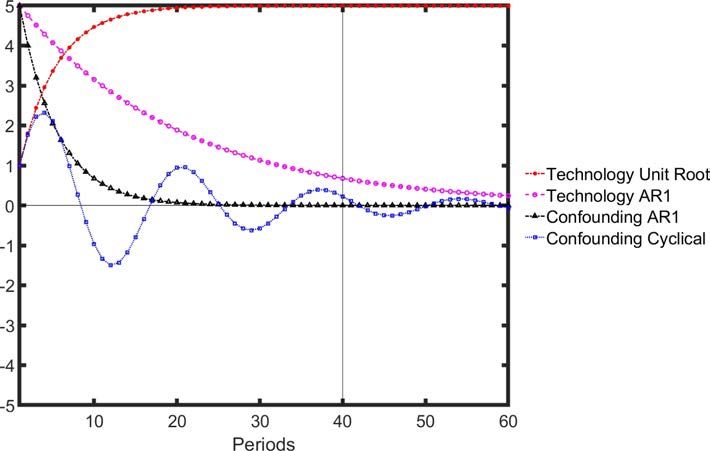
Abstract

       We address the identification of low-frequency macroeconomic shocks, such as technology,
       in Structural Vector Autoregressions. Whilst identification issues with long-run restrictions
       are well documented, we demonstrate that the recent attempt to overcome said issues using
       the Max-Share approach of Francis et al. (2014) and Barsky and Sims (2011) has its own
       shortcomings, primarily that they are vulnerable to bias from confounding non-technology
       shocks, although less so than long-run specifications. We offer a new spectral methodology
       to improve empirical identification. This new preferred methodology offers equivalent or
       improved identification in a wide range of data generating processes and when applied to US
       data. Our findings on the bias generated by confounding shocks also importantly extends to
       the identification of dominant business-cycle shocks, which will be a combination of shocks
       rather than a single structural driver. This can result in a mis-characterization of the business
       cycle anatomy.

Keywords: Identification, Long-Horizon and Business-Cycle Shocks, Confounding Shocks.
JEL classification: C11, C30, E32

ECB Working Paper Series No 2534 / April 2021                                                              1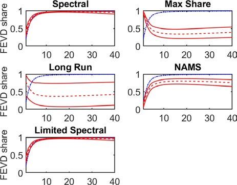
Non-technical summary

Structural Vector Autoregressions (SVARs) have increasingly been used to understand the dom-
inant drivers of both business-cycle and long-term fluctuations in the macroeconomy. Under-
standing these drivers can provide useful insights into important questions, such as whether
long-term productivity improvements come at the short-term cost of lower employment, or
whether the business cycle is predominantly driven by demand-side or supply-side factors.
This paper notes several theoretical shortcomings of existing SVAR identifications of dominant
drivers of business cycle and long-run economic fluctuations. This paper documents the biases
that can be introduced into the long-run and variance-maximizing methodologies by confound-
ing shocks, i.e. shocks other than the target of interest. Three alternative SVAR identifications
are proposed to deal with confounding shocks with different frequency domain properties, two
of which are new (Limited Spectral and NAMS). For identifying long-run shocks such as new
technological innovations, all proposed approaches and the Max-Share methodology are found to
be more robust to multiple sources of bias compared to the widely used ”long-run” identification
of technology shocks of Galı́ (1999).
Two types of SVAR identifications in the frequency domain show a further reduction in estima-
tion bias when identifying long-term shocks such as technology in the presence of business-cycle
frequency confounding shocks. The newly developed Limited Spectral identification also reduces
lag-truncation bias compared to existing spectral methodologies to a degree. These sources of
bias are shown to exist in data for the United States. The Spectral identifications are the only
methods able to both robustly estimate the SVAR using multiple data transformations suggest-
ing that they are the most appropriate identification method of long-term economic drivers such
as technology shocks.
This paper also illustrates a key weakness of variance-maximizing SVAR identifications of domi-
nant business-cycle shocks, such as the spectral approach at business-cycle frequencies. We show
that the identified shock will be a variance-weighted combination of many different business-
cycle drivers. Using a simple model, we show that recent research that has identified a non-
inflationary “main business cycle” shock is likely to instead be capturing a combination of infla-
tionary New-Keynesian style demand-drivers and deflationary positive supply shocks. The paper
demonstrates that caution should be applied in interpreting the results of variance-maximizing
methods in the frequency domain.

ECB Working Paper Series No 2534 / April 2021                                                   2
1     Introduction

    In this paper we revisit the use of Structural Vector Autoregressions (hereafter, SVAR) to identify
    dominant shocks, focusing on, but not limited to, its specific application to the identification of
    technology shocks.1 We examine the recently proposed solutions to address known drawbacks
    of the traditional long-run restriction by Francis et al. (2014) and Barsky and Sims (2011),
    through medium-run variance-maximizing identifications, and unearth a key weakness of these
    methodologies that have so far been under-explored but which have important consequences;
    notably, that these methodologies are likely to capture a range of shocks in addition to the target
    of interest. We suggest further modifications to the existing methods and point out the features
    of the data generating process that will result in the choice of one modification over another.
    In addition, these methods are also being used to identify dominant drivers of business-cycle
    macroeconomic developments (Angeletos et al., 2020; Levchenko and Pandalai-Nayar, 2018).
    We show that these applications can also suffer the same drawbacks due to confounding shocks,
    resulting in misleading conclusions being drawn.
        The use of SVARs to ‘look-through’ cyclical changes in productivity and isolate structural
    developments, or changes in technology, can be traced back to Blanchard and Quah (1989).
    In their approach, long-run restrictions are imposed in a structural VAR to separate the ef-
    fects of temporary ‘demand’ and permanent ‘supply’ shocks on GDP. This methodology was
    later adapted by Galı́ (1999) to specifically identify technology shocks in a two-variable VAR
    containing log-differences of productivity and hours worked.
        Long-run restrictions have been criticized on two main grounds, one economic and the other
    econometric: first, it is restrictive to assume that technology is the only shock that can affect
    productivity in the long-run;2 and second, econometrically, that imposing long-run restrictions
    on a finite sample and in the presence of non-technology shocks leads to biased and inefficient
    estimates. It is the second strand of the literature we investigate more deeply in this paper,
    notably the pitfalls of using alternative medium-run restrictions to identify long-run shocks. The
1
  We follow the literature and use ”technology” as a catchall phrase for the dominant long-run shock, while ”non-
  technology” represents the shocks with more fleeting effects.
2
  Several strands of research have suggested other non-technology shocks that may also result in permanent effects
  on labor productivity. Mertens and Ravn (2013) find that changes in taxation can have long-running effects of
  productivity, which once controlled for, lead to different dynamics of macroeconomic variables in response to
  identified technology shocks. Fisher (2006) separates productivity shocks into those that specifically apply to
  investment goods (IST shocks), and neutral technology shocks that affect aggregate production. In addition,
  Francis and Ramey (2005) and Uhlig (2004) have debated the extent to which the presence of these additional
  shocks alters the literature’s findings on the impact of technology shocks on hours worked.

    ECB Working Paper Series No 2534 / April 2021                                                               3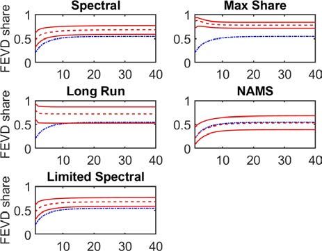
medium-run identification strategy is more robust to estimation on finite samples, identifying
technology shocks as those which contribute the most to the forecast error variance decompo-
sition (FEVD) of labor productivity at the 10-year horizon (Francis et al., 2014). We hereafter
refer to this approach as the ‘Max-Share’ identification. This strategy has also been used to
identify technology news shocks, which reflect changes in the perception of future long-run tech-
nology developments (Barsky and Sims, 2011).
    An important gap in the literature is how to identify technology shocks in the presence of
confounding shocks, a key feature of the data. One significant exception to this is Chari et al.
(2008), who find that long-run restrictions are only unbiased when technology shocks dominate
as a driver of output and non-technology shocks play a small role in a DSGE setting. In circum-
stances where non-technology shocks play a material role in driving macroeconomic variables,
long-run identifications will not only be biased, but will often show small and significant con-
fidence intervals around biased results — they will be ‘confidently wrong’ about the impact of
technology shocks. There is evidence that non-technology shocks are likely to play a larger role
in output fluctuations than commonly assumed, with estimates for the contribution of tech-
nology shocks to output ranging from just 2 to 63% of output variability (Galı́ and Rabanal
(2005), Christiano et al. (2003), Chari et al. (2008)). The issues raised by Chari et al. (2008)
for long-run identifications have yet to be raised for newer alternatives.
    We show that the Max-Share approach overcomes many of the weaknesses of long-run restric-
tions but can be biased by confounding non-technology shocks just as long-run identifications
can. We consider alternative approaches to sharpen the identification of technology shocks in
the presence of confounding shocks. The first, Non-Accumulated Max-Share (NAMS), shows a
lower degree of bias in the presence of low-frequency confounding non-technology shocks but is
susceptible to lag-truncation and short-sample bias. We next propose a spectral identification
approach whose rotation is in the frequency domain. Finally, we modify the spectral approach by
substituting the long-run variance-covariance matrix with one that can be reasonably obtained
in small samples. This preferred new methodologies is more robust to confounding shocks than
the Max-Share approach and is more robust to lag-truncation bias than existing methodologies
used to identify dominant shocks in the frequency domain (Angeletos et al., 2020; DiCecio and
Owyang, 2010).
    We highlight that the influence of confounding shocks and lag-truncation bias can have very
different effects even between two standard and relatively small-scale DSGE models. As an

ECB Working Paper Series No 2534 / April 2021                                                  4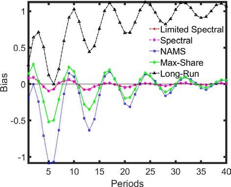
alternative, we employ a simple two-variable model that provides greater transparency around
the data-generating process than a DSGE model and removes the influence of lag-truncation
bias to demonstrate how the impact of confounding shocks can be dependent on their nature.
    Our findings have important implications for the identification of dominant business-cycle
as well as long-run macroeconomic drivers. Variance-maximising identifications have recently
been used to deconstruct the anatomy of business cycles. Specifically, Angeletos et al. (2020)
applied a similar identification concept at business cycle frequencies in an effort to determine the
possibility of a single shock driving the real side of the economy with little inflationary impact, in
contrast to the standard New Keynesian paradigm. We argue that confounding issues are more
acute at business-cycle frequencies and demonstrate the challenges they pose in determining the
true business cycle anatomy.
    The remainder of the paper is as follows: In section 2, we first revisit existing technology
identification methodologies, drawing attention to newly identified shortcomings of the Max-
Share and long-run approaches before outlining several proposed improvements. In section 3,
we then show the performance of each identification methodology in Monte Carlo simulations
on DSGE-generated data. We perform various experiments to identify the influence of varying
the importance of confounding shocks on each methodology, as well as the influence of short-
sample and lag-length limitations. In section 4, we simplify the data generating process by
using a simple 2-variable model to isolate the effects of different types of confounding shocks:
whether they drive low or business-cycle fluctuations in the data. This simplified model does
not have an ∞-representation, removing the influence of lag-truncation bias. In section 5, we
then take each specification to data for the United States, assessing which sources of bias are
likely impacting the identifications. Finally, we switch focus to demonstrate how confounding
shocks paint a different anatomical picture of business-cycle drivers than that proposed by recent
macroeconomic literature.

2     Empirical Approaches

In this section, we briefly revisit the standard long-run and Max-Share identification of a tech-
nology shock. The potential for the Max-Share approach to be contaminated by other non-
technology shocks is then explained, before we detail three approaches that can reduce contam-
ination, depending on its source.

ECB Working Paper Series No 2534 / April 2021                                                       5
2.1 Identifications and their Drawbacks
2.1.1 Long-Run Restrictions
We start with the simple and original approach that first introduced SVARs as a tool to dis-
entangle technology shocks from general macroeconomic fluctuations (Galı́, 1999). Isolating
the long-run components of labor productivity (prodt ) and total hours worked (hourst ), la-
beled LPLR and HoursLR , respectively, this methodology imposes the restriction that only the
technology shock can impact labor productivity in the long-run.
LPLR ∗ 0
tech.
= (1)
Hours ∗ ∗
LR non−tech.
Assuming the structural AR matrix polynomial,
A (L) = I2 − A1 L − A2 L2 . . . − Ap Lp (2)
The long-run counterpart is therefore,
A (1) = I2 − A1 − A2 . . . − Ap (3)
In a stationary VAR containing the log-difference series of productivity and hours, the long-
run effect of the technology shock on growth will dissipate. The long run impact of each shock
on the level of the target variable can be written as:
LPLR tech. tech.
Θ 0
= A(1)−1 = B(1)−1 A−1
0
= 11 tech. (4)
HoursLR non−tech. non−tec. Θ21 Θ22 non−tech.
where B(L) is the reduced-form VAR polynomial. Restricting the loading of the non-technology
shock onto productivity to be zero can be accomplished by ensuring the long-run impact matrix
is lower triangular. This is accomplished by solving for A−1
0 as follows:
−1 0
A−1
0 = B(1)chol[B (1) Σu B(1)−1 ] (5)
Where Σu is the reduced-form variance-covariance matrix.
ECB Working Paper Series No 2534 / April 2021 6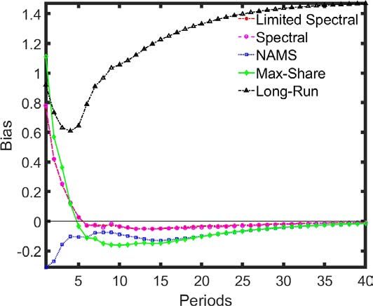
2.1.2      Max-Share

Long-run restrictions have come under fire for short-sample estimation problems and overly
restrictive assumptions. The Max-Share identification instead assumes that technology shocks
are the dominant driver of productivity around the 10-year horizon. In this identification, the
technology shock is that which drives the largest proportion of the forecast error variance of
labor productivity at this horizon, as in (Francis et al., 2014). When employing Max-Share one
has to be cognizant of the fact that at long horizons there are (cumulative) errors in the MA
coefficients on which the identification rests. These errors can be sizeable as argued in Lemma
1 below.

Lemma 1 VARs can produce increasingly biased and uncertain impulse responses as the horizon
increases. A simple argument illustrates this issue: For

                                                yt = φyt−1 + t                               (6)

the j th MA coefficient (impulse response) is Ψj = φj . This is a convex function of φ so Jensen’s
Inequality implies that E(φ̂j ) > [E(φ̂)]j . Even in cases where the OLS estimate of φ is biased
downward E(φ̂) < φ due to small-sample bias (Kilian, 1998), the implied estimate of Ψj could
be biased upward E(φ̂j ) > φj . As j gets large this bias can become enormous. Therefore, placing
restrictions at long(er) or infinite horizons can lead to severely biased impulse responses. In
addition, the uncertainty around estimates of Ψj will increase exponentially as the time horizon
of interest, j, increases. The function for the variance of the estimates for Ψj is again an
                                     j
increasing function of j, E( N1 N               j 2
                               P
                                i [φ̂i − [E(φ̂)] ] ), again due to Jensen’s inequality.

    Francis et al. (2014) surmise that 10 years is longer than the period over which the business
cycle occurs (typically assumed to be 2-8 years), but short enough to reduce challenges related
to estimation on a finite sample. This restriction is imposed in a VAR containing productivity,
hours, consumption and investment as a share of GDP. The forecast error at horizon k can be
written:

                                                         k−1
                                                         X
                                        yt+k − ŷt+k =          Dτ ut+k−τ                     (7)
                                                         τ =0

    Where D is a matrix of moving average coefficients. By defining an orthonormal matrix A0

ECB Working Paper Series No 2534 / April 2021                                                   7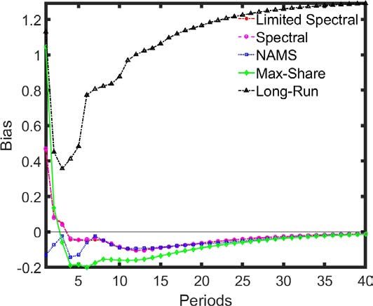
with columns α, and ϕ as a selection vector (size 1×n), we find the shock j which maximizes
the contribution to the total forecast error variance of variable i at horizon k
                                                      P
                                                       k−1 τ
                                            ϕ0i        τ =0 D αα0D
                                                                   τ0             ϕi
                           max f (α) =                P                              s.t. α0 α = 1   (8)
                                                           k−1 τ
                                                ϕ0i        τ =0 D Σu D
                                                                       τ0         ϕi

    Where ϕi is an indicator vector that selects the ith impulse response vector. The technol-
ogy shock at this maximized value is then: tech
                                            t    = α0 chol (Σu )−1 ut . Following Uhlig (2003),
identifying the structural shock that maximizes the contribution to the forecast error variance
of productivity is solved by identifying the eigenvector associated with the maximum eigenvalue
of Vτ , where Vτ is the FEVD of the target variable based on reduced-form shocks, and the
denominator of f (α).

                                                            k−1
                                                                                  !
                                                            X
                                         Vτ = ϕ0i                  D τ Σu D τ 0       ϕi               (9)
                                                            τ =0

2.2     Alternative Approaches

A drawback of the Max-Share approach is that in addition to capturing the long-run shock
of interest it also captures aspects of other shocks in the data. We propose three alternative
empirical approaches that offer reduced interference from these confounding shocks in different
circumstances.
    We first formally demonstrate the confounding nature of other shocks when using the Max-
Share identification. We present the key equations of the eigenvalue-eigenvector problem and
refer the reader to Appendix Section 8.1 for further details.
    Max-Share involves setting up the Lagrangian for Vτ :

                                         L(α) = α0 (Vτ )α − λ(α0 α − 1)

whose first order conditions reduce to solving for the eigenvector associated with the largest
eigenvalue of Vτ
                                                           Vτ α = λα

ECB Working Paper Series No 2534 / April 2021                                                           8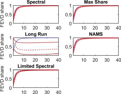
For a simple two variable VAR with the true structural coefficients of the form:
Al11 Ah12 l
A0 =
Al21 Ah22 h
where we use l and h to characterize the first shock as a low frequency (technology shock)
and the second as a high frequency (business cycle) shock. Given reduced form MA coefficient
counterparts, D, the solution for α at horizon k will be of the general form:3
Al11 + kτ=1 (Dτ11 Al11 +Dτ12 Al21 )
P
k
Ah12 + τ =1 (Dτ11 Ah12 +Dτ12 Ah22 )
P
α̃(k) =
1
In an attempt to isolate the low frequency technology shock, we can clearly see the po-
tential contamination coming from the high frequency shock as α depends on the initial im-
Al
h ), and their relative persistence:
pact of the respective shocks of the target variable (1) ( A11
Pk 12
(D11 Al11 +Dτ12 Al21 )
Pτk=1 τ11 h 12 h
. Essentially, the derived shock will not be of a ‘pure’ form, but rather a
τ =1 (Dτ A12 +Dτ A22 )
combination of shocks with the ratio dependent on their importance in driving the forecast er-
ror variance at the chosen horizon; if the high frequency shock has a sizeable initial impact this
will contaminate the identification more the shorter the identification horizon, while too long a
horizon will cause more uncertainty in the parameters. As the true form of A0 is unobserved,
the extent of this contamination in empirical applications is also unknown.
In general, there is no closed form solution to the eigenvalue-eigenvector problem and the
above expression is for an extremely special case where such a solution exists.4 However, we con-
sider this illustrative as the more complicated solution will exhibit the features of this restrictive
expression.
2.2.1 Non-Accumulated Max-Share (NAMS)
The standard Max-Share approach takes cumulative forecast errors up to time k: see equation 7.
As indicated above, and expanded in the Appendix, we show that there may be instances where
non-trivial proportions of the forecast error variance is driven by shocks of lower persistence
than the shock of interest.
The first methodology we propose will sharpen the identification of shocks with long-run
3
To satisfy the unit length restriction we will need to further normalize this by the length of the eigenvector.
4
For example, assuming the variance-covariance matrix is commutative at each horizon.
ECB Working Paper Series No 2534 / April 2021 9impacts by reducing the weight given to less persistent processes than technology. For example,
a high volatility AR(1) process with a small AR coefficient is also a predominantly low-frequency
process, but has no meaningful lasting impact at the 10-year horizon. As an alternative to Max-
Share, we propose finding the maximum of the square of the impulse response functions at a
particular horizon k. Here we aim to find the shock which has the maximum effects at say
period 40, ignoring all the previous horizon shocks. At this horizon, it may be expected that the
effects of lower-persistence shocks will have dissipated. The NAMS approach is implemented in
a similar way to the Max-Share approach, by solving:
ϕ0i Dk−1 αα0Dk−10 ϕi
k
max f (α) = s.t. α0 α = 1 (10)
ϕ0i (Dk−1 Σu Dk−10 ) ϕi
Kurmann and Sims (2017) also advocate reducing the impact of less persistent shocks in the
Max-Share approach. In the Barsky and Sims (2011) identification, the forecast error variance
under consideration is ‘double-weighted’; the maximization is applied to the summed forecast
error variance from periods 1 to k (max ki=0 f i (α), compared to the Francis et al. (2014) ap-
P
proach of max f k (α)). Kurmann and Sims (2017) propose returning to the original identification
of Francis et al. (2014), which maximizes a single forecast error variance at horizon k, finding
that it helps sharpen the identification of technology news shocks. Our NAMS approach takes
this to its logical conclusion, further reducing the distortion caused by transitory shocks.5
2.2.2 Spectral Identification
The NAMS approach deals with contamination from low-persistence, low-frequency processes.
However, the Max-Share approach may also be contaminated by driving processes that occur at
business-cycle and higher frequencies. Where the amplitude of these shocks are (coincidentally)
high at the chosen target range (k), the NAMS approach may not fare well.
We investigate the use of identification in the frequency domain, which can maximize the
share of variance explained only at frequencies that are of interest, excluding those that are
not. Identifying technology shocks through restrictions that explain the majority of low (long-
term) frequency volatility of productivity is a novel approach. However, this methodology has
in the past been used to assess the types of shocks which drive the business cycle. For example,
5
In addition, Uhlig (2004) suggests an identification in which non-technology shocks will have no effect after 10
years, such that technology shocks can be identified by a restriction such that only the technology shock has an
impact on productivity at that horizon. Our approach differs in that we do not exclude other shocks from having
an effect at this horizon, and instead look for the shock that dominates at 10-years.
ECB Working Paper Series No 2534 / April 2021 10Angeletos et al. (2020) find that a single shock drives the majority of the variance of a range
of macroeconomic variables at business cycle frequencies. DiCecio and Owyang (2010) use the
spectral approach to conduct an identification of technology shocks that is similar to what we
propose in this article but do not evaluate its performance.6 We effectively apply a band-
pass filter using the reduced form coefficients of a VAR containing macroeconomic variables,
identifying the spectral density of the variables within a particular frequency band. We then
identify the technology shock by maximizing the variance of productivity explained at the desired
frequency.
The spectral density of series Y at frequency ω can be written as a Fourier transform of its
auto and cross covariances (γ) at lag τ :
Z ∞
SY Y (ω) = γ (τ ) e−iτ ω (11)
τ =−∞
Therefore, once γ(τ ) in known, the spectrum, SY Y (ω), can be straightforwardly calculated.
The reverse also holds. That is, knowing the spectrum, SY Y (ω), leads to an easy computation
of γ(τ ) by using the inverse Fourier transform,
Z π
γ(τ ) = eiτ ω SY Y (ω)dω (12)
−π
Setting τ = 0, gives the variance of the time series Y .
Z π
γ(0) = SY Y (ω)dω (13)
−π
This means that the variance of Y is the integral of the spectrum over all frequencies, −π <
ω < π. This further indicates that the spectrum decomposes the variance of Y into components
from non-overlapping frequencies. Therefore, similar to the Max-Share identification, spectral
analysis allows us to gauge the importance of cycles at different frequencies to the variance of the
series of interest. And importantly, we can remove unwanted frequencies from the maximization
problem.
To employ this methodology we first need to uncover a VAR representation of the spectral
density of Y. We start by writing the Wold representation of the VAR (assuming it is invertible):
6
In addition, Christiano et al. (2006) find that by using a spectral estimator at frequency 0, Long-run restriction
estimates prove less biased following a MCMC assessment of VAR performance.
ECB Working Paper Series No 2534 / April 2021 11−1
Yt = I − B1 L + B2 L2 + . . . Bp Lp ut = Dut (14)
By post-multiplying Yt by Yt−τ and summing across its lags (of τ periods), the series of auto
and cross covariances can be discretely approximated by:
∞
X ∞
X
γ (τ ) = EYt Yt−τ = DΣu D0 (15)
τ =−∞ τ =−∞
−1
Then, by writing D e−iτ ω = I − B1 Le−iω + B2 L2 e−i2ω + . . . Bp Lp e−ipω
, the spec-
tral density of Y can be written as a function of the reduced-form VAR coefficients.
∞
iτ ω 0
X
−iτ ω
γ (τ ) e−iτ ω
SY Y (ω) = D e Σu D e = (16)
τ =−∞
To assess the spectral density within a frequency band, the spectral power can be integrated
between the bounds of the frequencies of interest [ω , ω̄]
As in the case of the Max-Share approach, the shock which maximizes the contribution to the
variance of productivity over this band is the eigenvector associated with the largest eigenvalue
R ω̄
of the matrix ω SY Y (ω). To identify technology, the band of interest is restricted to frequencies
below (longer-than) 10 years, to exclude business-cycle frequencies.
2.2.3 Limited-Horizon Spectral Identification
One criticism that can be leveled against the spectral identification approach is that the long-run
VAR representation used to calculate the spectrum of the endogenous variables may be biased
when estimated on a short sample of data and with limited lags.
Simulation exercises in section 3.2.2 demonstrate that biases in the impulse responses of long-
run restricted models get larger and larger with the response period, even where large numbers
of lags are included in the estimation. This is especially true for reasonably lagged VARs (10
lags or below; those typically estimated with macro-data). At shorter horizons the responses
are closer to the truth. Our proposal, therefore, is to use projections extending to 10 years (as
in the original Max-Share approach) rather than the long-run representation. This horizon is
long enough to capture the theoretical underpinning of the structural identification but short
enough to reduce the degree of ”lag-truncation” bias.
A “windowed” selection of autocorrelations is often used to estimate the spectrum of a series.
ECB Working Paper Series No 2534 / April 2021 12The same principle can be used in the spectral VAR identification process, effectively applying
a truncated kernal estimation approach. For example, the infinite-MA representation, D(eiω )
can be replaced with a limited horizon series of impulse response coefficients.
k−1
X
−iτ ω
D (e k
)= Dτ e−iτ ω (17)
τ =0
The same process used in the standard spectral approach is also used to identify the shock
of interest. For example, identifying technology shocks as the dominant drivers of labor pro-
ductivity over frequencies below 10 years. Additionally, as will be shown subsequent sections,
in DSGE models with infinite-order representations, and seemingly the US data, short-samples
of data and a limited number of lags can result in a larger bias to identifications that rely on
the infinite-order MA representation. The Limited Spectral methodology, like the Max-Share,
is less susceptible to this bias.
3 DSGE Model Evaluation
Traditionally, SVARs seeking to extract an unobservable shock, such as technology, have been
evaluated on their performance using simulated data from a DSGE model (Barsky and Sims,
2011; Chari et al., 2009; Erceg et al., 2005; Francis et al., 2014). This is an intuitive exercise, given
that the true underlying shock is known by construction. In this section, we test our estimators
with two known data-generating processes, a New-Keynesian model and a Real Business Cycle
model. We argue that many of these tests have been performed using calibrations of these DSGE
models which fail to test for the influence of material confounding shocks needed to replicate
key features of US macroeconomic data. We later show that existing methodologies perform
poorly when these features are included in simulated data from a simple 2-variable model that
provides greater transparency over the data-generating process compared to a DSGE model.
Each VAR specification is first tested on a standard medium-scale New Keynesian model,
of the type proposed by Christiano et al. (2005), and used by Francis et al. (2014) and Barsky
and Sims (2011) to evaluate their respective implementations of the Max-Share identifications.7
This model contains features such as persistent consumption habits, investment adjustment
costs, capital utilization, and partial price and wage indexation (see Appendix 8.2). In addition,
7
In the Barsky and Sims (2011) ‘news’ implementation of the Max-Share identification, an additional ‘news’ shock
is added to the standard medium-scale NK model, which affects technology with a lag of one period.
ECB Working Paper Series No 2534 / April 2021 13we also test the SVAR identifications on the RBC model used in Chari et al. (2008).
3.1 New Keynesian and RBC Monte-Carlo DSGE Results
A standard shock calibration is used to test each VAR specification on both the New Keynesian
and RBC DSGE models. The first follows the calibration of Erceg et al. (2005), while the
second follows the baseline calibration of Chari et al. (2008). The results below are based
on 1000 simulations of each DSGE model, generating 250 observations after a burn-in of 100
periods. Each VAR is estimated via a Gibbs sampling procedure with flat priors, saving 1000
draws following a 500-period burn-in. The same procedure is used for all simulations throughout
the document.
For the New Keynesian simulation, a four-variable VAR is estimated using: the natural logs
of productivity, total hours worked, and the share of investment and consumption in GDP. For
the RBC model, a two-variable VAR is estimated on the log-level of productivity and hours
worked. For the long-run identification, log-differenced productivity is always used, as is stan-
dard. However, to demonstrate the effects of confounding shocks with different transformations
of the data, we estimate the other SVARs (Max Share, NAMs, and Spectral methods) with
productivity in both log-levels and log-differences.
Figure 1: IRF bias of technology shock on productivity, estimation on log-level of produc-
tivity: NK and RBC models
New Keynesian RBC
Note: Long-run estimation performed using labor productivity in log-differences.
ECB Working Paper Series No 2534 / April 2021 14Labor productivity in levels: Figure 1 plots the biases of the impulse response of labor
productivity to a technology shock when productivity is specified in levels (except the Long-
Run SVAR). For both models, the Spectral, Limited Spectral, and Max-Share identifications
have similar performances, showing the least bias for the initial response periods. However,
their relative performance decays monotonically relative to NAMS. In both models NAMS has
relatively high initial bias but its rate of decay is slower than that of the other estimators.
The slower decay means that at longer horizons there is little distinction between the relative
performance of all the estimators. At earlier horizons, the Limited Spectral and Max-Share
identifications show slightly lower bias than the Spectral identification, which we will later
argue is due to lower susceptibility to lag-truncation bias.
Figure 2: IRF bias of technology shock on productivity, estimation on differenced produc-
tivity: NK and RBC models
New Keynesian RBC
Labor productivity in log-differences: In the NK model, the Long-Run identification,
estimated with productivity in log-differences, showed a lower degree of bias at medium to long
horizons than the other estimation methods, estimated using the level of log-productivity (see
left panel of Figure 1). However, when we estimate the models with productivity in differences
for all specifications, there are clear patterns that emerge with respect to the degree of bias (see
Figure 2). In both models, the Spectral, Limited Spectral and Max-Share again show similar
level of bias across the response horizons. In the NK model, each of these identification have
biases of the same sign and are best at recovering the true impulse responses of the DSGE
ECB Working Paper Series No 2534 / April 2021 15models. However, in the RBC model, NAMS displays the least initial bias (in absolute value)
but quickly decays for medium to long horizons. The four remaining methods (Max-Share,
both Spectral, and Long-Run identifications) have similar absolute initial biases, negative for
long-run and positive for the others. After horizon 30 all four display the same bias, in sign and
magnitude.
Summary: The consistently high-performing SVARs in both simulations in the early pe-
riods of the IRF are the Max-Share, Spectral and Limited Spectral identifications. The shocks
uncovered by the VARs have a high correlation (over 0.9) with the true underlying technol-
ogy shock, corresponding to the low IRF bias for these specifications (Table 1). These three
identifications also show lower degrees of bias in estimations of the impact of technology on
hours-worked (Appendix 8.2). By period 30 of the IRF, the Max-Share, Spectral, Limited Spec-
tral, and Long-Run identifications show similar biases in both models, with the exception of
the Long-Run restriction in the New Keynesian case. When they are all estimated using labor
productivity growth, the three aforementioned identifications outperform the Long-Run identifi-
cation for at least the first 5-years of the response period. The NAMS specification has a higher
IRF bias than the Max-Share, both Spectral specifications, and the Long-Run identifications
in most cases. We surmise that this is mainly due to the fact that NAMS is estimated using
parameters only at horizon 40 when the errors in estimation would have accumulated to sizeable
degrees (see Lemma 1, and, as we will argue below, also due to the presence of lag-truncation
bias).
Table 1: Correlation of VAR-identified technology shocks with true DSGE-generated shock
Identification Max-Share Long-Run Spectral Limited Spectral NAMS
New Keynesian 0.90 0.85 0.90 0.90 0.77
(0.70, 0.96) (0.53, 0.96) (0.64, 0.96) (0.67, 0.96) (0.43, 0.95)
RBC 0.97 0.86 0.96 0.97 0.95
(0.86, 0.99) (0.74, 0.94) (0.84, 0.99) (0.86, 0.99) (0.80, 0.99)
Note: 5th and 95th percentile values shown in brackets.
The high performance of our estimators in levels in matching the true IRFs at early horizons
is likely to be in part due to the shock processes driving the DSGE model, and the degree to which
they drive the volatility of the simulated data (levels and differences). The highly persistent
technology shock in this and other similar DSGE models tends to drive the vast majority of
the variance of labor productivity. In this calibration, over 99% of the volatility of the level of
ECB Working Paper Series No 2534 / April 2021 16labor productivity in both models is driven by the technology shock.8 Therefore, several of the
methodologies find a similar result given how insignificant the non-technology driving processes
are in the variation of productivity.
The high performance of said estimators when using labor productivity growth is likely due
to the technology shock lingering over time via the capital accumulation process. Notice that
the relative performance of the three highest performing estimators (Max-Share, Spectral and
Limited-Spectral) are even more pronounced in the NK DSGE model, where non-technology
shocks display significantly smaller initial impacts on labor productivity (and therefore growth
rates) than in the RBC specification (Figure 3). In contrast, the initial impact of the non-
technology shock is almost as large as technology in the RBC model, resulting in larger biases.
Figure 3: Productivity IRFs for all shocks in New Keynesian and RBC models
New Keynesian RBC
When applied to US data we find that, unlike in the DSGE models, the impulse response of
Max-Share differs significantly from those produced by the spectral methods when productivity is
specified in differences. Our explanation of this finding rests on the DSGE models not containing
the types of non-technology confounding factors as the data. This elucidates our earlier premise
that Max-Share has even more difficulty (than spectral methods) disentangling technology shocks
from persistent non-technology confounding shocks (see also section 4.1 for further illustration
of this point).9 Therefore, when the nature of the confounding shock contributes non-trivially to
8
Based on re-simulating the model over 100,000 periods one shock at a time.
9
See Sala (2015) who also estimate a New Keynesian DSGE model in the frequency domain. Also, Fernald (2007)
found significant low frequency components in US productivity growth.
ECB Working Paper Series No 2534 / April 2021 17the dynamics of productivity the method used to identify technology becomes especially important.
Arguably, the standard DSGE specification does not adequately ’road-test’ the performance
of the VARs in a transparent way. In the following sections, we first examine VAR performance
in the event that larger confounding shocks drive a more material component of the data process
than assessed in traditional DSGE models. We address this issue by stripping away the complex-
ities of the transmission mechanisms of our DSGE models and examine the performances of our
SVAR estimators under a variety of non-technology confounding shocks in a simple two-variable
setting. However, before doing so we address two important criticisms by Chari et al. (2008)
(hereafter, CKM) levied against long-run identification using the RBC model, concerning the
size of confounding shocks (but not their nature) and the impact of lag-truncation bias.
3.2 Addressing the CKM Critique of SVARs
In this section, we directly address two issues raised by Chari et al. (2008) about long-run
identified SVARs: IRF bias with a varying importance of non-technology shocks, and IRF bias
when the true lag length is infinity and is not imposed in estimation (lag-truncation bias).
Chari et al. (2008) use the above-discussed RBC model to demonstrate the difficulties faced by
long-run restricted SVARs in capturing technology shocks as other non-technology confounding
shocks drive an increasing share of the variance in the model. We therefore test our proposed
identification methodologies against this known DGP with which long-run restrictions are shown
to have difficulty. We show that our new methodologies generally outperform the long-run
identification SVAR, and perform comparably with the Max-Share identification in this RBC
DSGE framework.
In this model, there is no advantage of using the new specifications above those offered by the
Max-Share approach. The reason is that the non-technology shock has low-frequency properties
(it is an AR(1) process), and therefore can confound the spectral as well as the Max-Share
identifications. However, we demonstrate that compared to the long-run restriction approach,
all other specifications show lower, or at least equal, degrees of bias. In subsequent sections,
we show that there are circumstances where labor productivity is influenced by other types of
confounding shocks where our new identifications outperform both the long-run and Max-Share
identifications. Therefore, in contrast to the findings of CKM, when using the right estimator,
SVARs can prove useful in identifying the impacts of technology shocks for a range of DGPs.
The RBC model is specified with a unit root for technology, but also a highly volatile and
ECB Working Paper Series No 2534 / April 2021 18persistent non-technology shock τ , where it’s persistence ρl is 0.95 in the standard calibration.
Chari et al. (2008) note that two sources of bias exist for the long-run SVAR methodology:
non-technology shocks will increase IRF bias as they drive a larger proportion of the variance
of output; and lag-truncation bias, where limited VAR lags result in a bias due to the true
specification of the VAR having an ∞-representation.
3.2.1 Varying the Relative Importance of Structural Shocks
Turning to the first claim, the relative variance of the non-technology shock to the technology
σ2
shock is adjusted ( σ2lt ) and the model is simulated 1000 for each ratio of variance, generating
zt
a data sample of 180 periods for each relative variance combination.10 Each VAR is estimated
using 4 lags. The long-run SVAR is estimated with log hours specified as ht −αht−1 , where α de-
termines the degree of quasi-differencing, as in CKM. This allows the VAR to be estimated with
total hours in both levels and a highly quasi-differenced form.11 All other SVAR specifications
use hours in levels.
This exercise has a direct link to the eigenvalue-eigenvector rotation of variance-maximizing
identifications. Recall the discussion in Section 2.2 where it was pointed out that success of
Max-Share rotation, from reduced form to structural space, depends on the relative importance
of the impact of the technology and non-technology shocks in driving the FEV at the targeted
horizon.
Productivity in Levels:
We draw the following conclusions from Figure 4:
• The long-run IRF for productivity is ‘confidently wrong’ (also demonstrated by Chari et al.
(2008)) when the non-technology shock generates over 50% of the variance of output in the
model in the quasi-differenced long-run specification. The specification with hours in levels
has the largest bias and confidence intervals of the remaining specifications. However, the
Max-Share and our new approaches correctly display uncertainty in the identification of
technology shocks, via wider error bands, as the non-technology shock variance increases.
See Christiano et al. (2007) for a discussion of large confidence intervals relative to the
size of the bias in the context of Chari et al. (2008).
10
The standard Gali calibration used to create Figure 1 in Chari et al. (2008) is used.
11
Two specifications are used, with hours in levels (α = 0) and hours with a high-degree of quasi-differencing
(α = 0.99).
ECB Working Paper Series No 2534 / April 2021 19Figure 4: CKM: Impact coefficient bias on labor productivity IRF as proportion of output
driven by non-technology shock is varied
Note: The proportion of variance driven by the non-technology shock is calculated by simulating the model with
one shock at a time, and then comparing the variance of the HP-filtered series for output from each simulation,
as in CKM.
• The Max-Share, Limited-Spectral and NAMS approaches show smaller confidence bands
than the Spectral methodology. These specifications do not rely upon the infinite MA
ECB Working Paper Series No 2534 / April 2021 20representation, but instead use a finite representation. Their error bands are therefore
smaller, reflecting a more efficient estimation.
• Our alternative methodologies show lower bias than the long-run identification as the non-
technology shock increases in size. However, the Max-Share identification is marginally
more efficient than the spectral approach, showing slightly less bias at all horizons. The
NAMS identification becomes more biased as the non-technology shock grows larger in
importance. Reducing the persistence of the non-technology shock relative to the CKM
specification reduces this bias however (Appendix 8.4).
Figure 5: CKM estimated on differenced productivity: Impact coefficient bias on labor
productivity IRF as proportion of output driven by non-technology shock is varied
Note: The proportion of variance driven by the non-technology shock is calculated by simulating the model with
one shock at a time, and then comparing the variance of the HP-filtered series for output from each simulation, as
in CKM. This chart shows the contribution of output variability to the level of labor productivity for consistency
with figure 4
ECB Working Paper Series No 2534 / April 2021 21Productivity in Differences: In figure 5:
• The Max-Share and Spectral identifications show very similar degrees of bias to the highly
quasi-differenced long-run specification. However, in section 4.1, we show that over longer
horizons, beyond the initial impact periods, the Spectral approaches show considerably
lower biases relative to the long-run and Max-Share identifications.
• The NAMS approach incorrectly captures the non-technology shock to a high-degree and
a large number of draws show the effect on labor productivity falling close to zero. This
can be intuitively understood: the effect of the technology shock on labor productivity
growth is close to zero at the 10-year horizon, such that disentangling the two shocks is
difficult for this methodology. In section 5, this is found to be a feature of the US data.
3.2.2 Lag-Truncation Bias
In the second exercise, we examine the robustness of each methodology to lag-truncation bias.
This is the bias caused by estimating the VARs using a finite number of AR coefficients when the
true DSGE-generated data has an infinite-lag order. There are two main findings from running
each method on 100,000 simulated data points from the RBC model and varying the number of
lags used in the estimation (Figure 6).
• At low lag levels, alternate methods show lower initial bias relative to the long-run spec-
ification. Further out, at long horizons, the new specifications show a similar bias to the
long-run identifications.
• The NAMS and Spectral specifications continue to show more bias than the Limited Spec-
tral and Max-Share specification on impact. The Spectral methodology is dependent on
the long-run VAR representation, while the NAMS approach identifies the shock maximiz-
ing the variance at a long-term horizon (10-years), where the effects of lag-truncation bias
are larger than in earlier periods of the IRF.
ECB Working Paper Series No 2534 / April 2021 22Figure 6: CKM: IRF bias as estimation lag-length is varied
Note: Estimation on 100,000 periods of data simulated using the CKM RBC model, varying the number of lags
used to estimate each SVAR. The relative variance of the technology and non-technology shocks are held constant,
2
σnon−technology
at 2
σtechnology
= 0.64, as in CKM.
ECB Working Paper Series No 2534 / April 2021 234 An Illustrative Two Variable Data-Generating Process
Here we examine how the VARs perform when the data generating process is a more transparent
set of technology and non-technology shocks. It is useful to strip away the complexity of the
dynamics driven by the DSGE model so that we can clearly examine how different data processes
can affect the results.
To that end, a simple two-variable model is used to generate the data. Figure 7 provides a
stylized example of the different forms a traditional technology shock can take, from a persistent
AR(1) to a unit-root shock. We test both forms in the scenarios below. In contrast, non-
technology shocks to productivity, such as less persistent AR(1) and cyclical business-cycle-
related shocks, may also be in the data, driving a material proportion of the variance. In a second
simplifying assumption, the DGPs considered here do not have an infinite lag specification,
therefore we abstract from the issues associated with lag-truncation bias.
Figure 7: Stylized IRFs for technology shock to productivity and confounding shocks
4.1 The Case of Unit Root Technology Shocks
We start by testing the identification of technology shocks in a simplified two-variable model
where technology shocks take the form of a unit root process with a persistent growth component.
This allows us to replicate the slow-building effect of technology shocks on labor productivity as
in the DSGE models. This is also likely to be a key feature of the US data, as we will show. In
contrast to the DSGE models previously explored, the confounding non-technology shock will be
ECB Working Paper Series No 2534 / April 2021 24both high-volatility, and high (-er) persistence. This will allow us to replicate sharply differing
results for the Max-Share and spectral methodologies that we find in US data.
A simple two-variable data process is generated for labor productivity (L) and hours (N ).
g
Both processes are driven by a technology shock (z ) and a non-technology shock (b ). The
two-variable model takes the form:
Lt = ztl + bt (18)
Nt = 0.7Nt−1 − 0.3Nt−2 − 0.3z l + 0.3bt (19)
ztl = zt−1
l
+ ztg (20)
g
ztg = ρz g zt−1
g
+ zt (21)
bt = ρb,1 bt−1 + bt (22)
g
The technology shock zt is a permanent shock to the level of productivity L, with persistent
effects on its growth rate. bt provides a temporary impact on the level of productivity. We
choose an illustrative calibration where the non-technology shock has a higher volatility but
g
lower persistence than the technology shock (σ b = 2, ρb = 0.3, σ z = 1). The parameter ρz g ,
which governs the persistence of the effect on productivity growth, is set to 0.8, a reasonable
value.12
Given that we are interested in the particular case of a shock process driving the growth rate
of productivity, we estimate each of the VARs in both levels and differences for productivity. In
the first case, where the VARs are estimated on the differenced labor productivity series (L),
the Spectral approaches show the lowest level of bias in their IRFs (Figure 8). In contrast, the
Max-Share and long-run identifications show very high-levels of bias, taking on many of the
properties of the non-technology shock.
To see why this is the case, observe that the differenced series L is the sum of the differenced
series z l and b (∆Lt = ∆ztl + ∆bt ). The first term is simply the low frequency AR(1) process
g
∆z l = ztg = ρz g zt−1
g
+ zt
12
Lindé (2008) finds the persistence parameter to be low (0.14) but the variance of z g to be high - he also finds the
model fit was also very good when ρzg was high but var(z g ) was low.
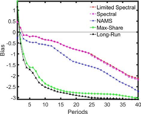
ECB Working Paper Series No 2534 / April 2021 25Figure 8: IRF bias where technology growth has a unit root
Differences estimation Levels estimation
Note: The long-run specification requires the productivity data to be estimated in log differences. The results
for the bias of the long-run specification in ’levels’ plot reports the estimation in log differences for comparison
purposes.
while the second reduces to
∆bt = (ρb − 1)bt−1 + bt
As (ρb − 1) is negative, this second process is a mixture of high frequency and white noise
processes. This may contribute to the volatility of ∆L but does not have persistent low-frequency
effects. The Max-Share identification is, therefore, less capable of distinguishing between this
and the true persistent technology shock. The Spectral approaches assign most weight to the low-
frequency persistent shock, as does the NAMS approach, which ‘looks through’ the transitory
white noise and high-frequency process resulting from differencing b. However, it is clear that
the dominance of the technology shock in growth rates will fade as the persistence of the growth
shock, ρz g , falls. An exercise in which this parameter is reduced to 0.3 from 0.8 shows a severe
deterioration in performance for the spectral approaches, although they continue to have the
lowest bias on impact.
The ability of the Spectral and NAMS identifications to distinguish between these data
generating processes also enables them to more accurately estimate the proportion of forecast
error variance of productivity driven by the technology shock (Figure 9). When estimating the
VAR in levels, we find that all approaches have a similar performance with the exception of
the long-run restriction - which is always estimated in differences but shown for comparison
ECB Working Paper Series No 2534 / April 2021 26Table 2: Correlation of VAR-identified shocks with true technology shock when
technology has a unit root
Identification Max-Share Long-Run Spectral Limited Spectral NAMS
Differenced 0.31 0.23 0.96 0.96 0.96
(0.10, 0.46) (-0.04, 0.63) (0.89, 0.98) (0.89, 0.98) (0.92, 0.98)
Levels 0.97 NA 0.97 0.97 0.97
(0.93, 0.99) NA (0.93, 0.99) (0.93, 0.99) (0.83, 0.99)
Note: The long-run specification requires the productivity data to be estimated in differences in both cases. 5th
and 95th percentiles shown in brackets.
Figure 9: Estimated FEVD where technology growth has a unit root
Differences estimation Levels estimation
Note: 5th and 95th percentiles in brackets
purposes with levels results - (Figure 9 and Table 2). This accuracy is driven by all approaches
accurately estimating the initial variance of the technology shock. However, the IRFs under all
approaches are less accurate relative to those estimated by the Spectral VARs on the differenced
data. Effectively, the additional dynamics in productivity growth driven by the technology shock
are obscured when estimating the VAR with the data in levels. As such, the IRFs prove less
persistent than the estimates of the Spectral and NAMS VARs on differenced productivity, and
further away from the true persistence of the shock.
4.2 The Case of Stationary Technology Shocks
In the unit root case, the confounding non-technology shocks simply took the form of a less
persistent, albeit also low-frequency shock. The form of the confounding shock was a secondary
ECB Working Paper Series No 2534 / April 2021 27point, since the unit-root shock dominated the variance of observable variables, as in the New
Keynesian and RBC models under consideration. There will however be situations in which
the shock targeted by the econometrician is less clearly dominant in the DGP. This may occur
for some economies subject to large non-technology shocks, or even when the econometrician is
targeting shocks other than technology.
In this section, the model is further simplified so that the technology shock is no longer as
clearly dominant in driving the variance of the model, and instead takes the form of an AR(1)
process. The form of the confounding shock gains importance in these simulations. We now
allow our confounding non-technology shock to take two forms: a low-frequency shock of the
same form as the technology shock, but less persistent, and a second business-cycle frequency
process.
Again, a simple two-variable data process is generated for labor productivity (L) and hours
(N ). Both processes are driven by a technology shock (z ) and a business-cycle shock (b ).
Lt = zt + bt (23)
Nt = 0.7Nt−1 − 0.3Nt−2 − 0.3zt + 0.3bt (24)
zt = 0.9zt−1 + zt (25)
bt = ρb,1 bt−1 + ρb,2 bt−2 + bt (26)
This simple process is calibrated to replicate some of the features of a more complex model,
while being more transparent. In the case of a technology shock, labor productivity rises persis-
tently, while hours-worked initially falls (as in the New Keynesian framework). The advantage
of this simple setup is that we can change the driving processes of the non-technology shock
through the ρb parameters and easily understand how this changes the properties of the data
and hence the estimation performance of the VAR specifications.
4.2.1 Motivating the Choice of Stochastic Processes
We choose our shock processes to examine two plausible scenarios in the detection of technology
shocks:
1. There are confounding low-frequency but less persistent processes in the data other than
ECB Working Paper Series No 2534 / April 2021 28You can also read