WP/17/223 Building Resilience to Natural Disasters: An Application to Small Developing States - International ...
←
→
Page content transcription
If your browser does not render page correctly, please read the page content below
WP/17/223

                           Building Resilience to Natural Disasters:
                          An Application to Small Developing States

                        by Ricardo Marto, Chris Papageorgiou, and Vladimir Klyuev

IMF Working Papers describe research in progress by the authors and are published to
elicit comments and to encourage debate. The views expressed in IMF Working Papers
are those of the authors and do not necessarily represent the views of the IMF, its Executive
Board, or IMF management.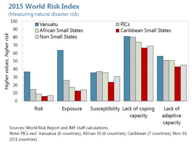
© 2017 International Monetary Fund                                                                   WP/17/223

                                           IMF Working Paper
               Research Department and Strategy, Policy, and Review Department

    Building Resilience to Natural Disasters: An Application to Small Developing States*

           Prepared by Ricardo Marto, Chris Papageorgiou, and Vladimir Klyuev

                           Authorized for distribution by Chris Papageorgiou

                                                 October 2017

IMF Working Papers describe research in progress by the author(s) and are published
to elicit comments and to encourage debate. The views expressed in IMF Working
Papers are those of the author(s) and do not necessarily represent the views of the IMF, its
Executive Board, or IMF management, or U.K. DFID.

                                                    Abstract

We present a dynamic small open economy model to explore the macroeconomic impact of
natural disasters. In addition to permanent damages to public and private capital, the disaster
causes temporary losses of productivity, inefficiencies during the reconstruction process, and
damages to the sovereign's creditworthiness. We use the model to study the debt sustainability
concerns that arise from the need to rebuild public infrastructure over the medium term and
analyze the feasibility of ex ante policies, such as building adaptation infrastructure and fiscal
buffers, and contrast these policies with the post-disaster support provided by donors. Investing
in resilient infrastructure may prove useful, in particular if it is viewed as complementary to
standard infrastructure, because it raises the marginal product of private capital, crowding in
private investment, while helping withstand the impact of the natural disaster. In an application
to Vanuatu, we find that donors should provide an additional 50% of pre-cyclone GDP in grants
to be spent over the following 15 years to ensure public debt remains sustainable following
Cyclone Pam. Helping the government build resilience on the other hand, reduces the risk of
debt distress and at lower cost for donors.

JEL Classification Numbers: E22, E62, F34, F35, H54, H63, H84, O23, Q54.
Keywords: Natural Disastes, Resilience, Adaptation, Debt Sustainability, Small States.
Authors’ E-Mail Addresses: rmarto@imf.org, cpapageorgiou@imf.org, vklyuev@imf.org.

*
  Authors are grateful to seminar participants at the IMF for their useful comments, suggestions, and advice.
This working paper is part of a research project financed by the U.K.'s Department of International
Development (DFID) to support macroeconomic research on Low Income Countries. The views expressed in
this paper are those of the authors and do not necessarily represent those of the IMF, or of IMF policy, or of
DFID.
Contents
Page
1. Introduction 3
2. The Model 6
3. Calibration 12
4. Recovering with Fiscal and Debt Sustainability 18
4.1. Alone in the Dark . . . . . . . . . . . . . . . . . . . . . . . . . . . . . . . . . . . . . . 18
4.2. Grants for Reconstruction . . . . . . . . . . . . . . . . . . . . . . . . . . . . . . . . . 19
5. Building Resilience with Adaptation Infrastructure and Fiscal Buffers 20
5.1. Investing in Resilient Infrastructure . . . . . . . . . . . . . . . . . . . . . . . . . . . . 20
5.2. Building Fiscal Buffers . . . . . . . . . . . . . . . . . . . . . . . . . . . . . . . . . . . 21
6. Conclusions 24
References 26
Figures
Figure 1: One of the most at risk countries . . . . . . . . . . . . . . . . . . . . . . . . . 4
Figure 2: The natural disaster’s transmission channel . . . . . . . . . . . . . . . . . . . . 15
Figure 3: Debt and fiscal sustainability implications . . . . . . . . . . . . . . . . . . . . 19
Figure 4: More resilient infrastructure, lower damages . . . . . . . . . . . . . . . . . . . 21
Figure 5: Resilient infrastructure reduces risk of debt distress . . . . . . . . . . . . . . . 22
Figure 6: Saving in a contingency fund helps smooth the recovery . . . . . . . . . . . . . 23
Tables
Table 1: Selected initial values (%) . . . . . . . . . . . . . . . . . . . . . . . . . . . . . . 16
Table 2: Calibrated parameters . . . . . . . . . . . . . . . . . . . . . . . . . . . . . . . . 17
23
1. Introduction
Small developing states are among the most vulnerable countries in the world to natural disasters
and climate change. The UN World Risk Index, which measures exposure to natural hazards and
the capacity to cope with these events across 171 countries, places small developing states at the top
of its ranking. In addition to the limited capacity to respond to natural disasters, these countries
are more frequently hit by extreme weather events than larger countries and their economic costs
are on average much larger (IMF, 2016a). Climate change will only worsen the reach of natural
disasters, by increasing their intensity and frequency (IPCC, 2014). This vulnerability to natural
disasters exacerbates the challenging tradeoff policymakers face domestically—allocating spending
for growth-promoting infrastructure or vulnerability-reducing resilience—and externally by the donor
community—allocating financial support pre or post-disaster.
Boosting infrastructure investment has gained renewed attention as an imperative for economic
development. It encourages private investment and increases productivity, and fosters inclusion by
improving connectivity and allowing people to spend their time on more productive activities. Improv-
ing infrastructure is indispensable for attaining the Sustainable Development Goals and it is regularly
included as a key pillar of countries’ national development strategies. Particularly important in this
context are the links between infrastructure and climate change. The links run in two directions. First,
certain types of infrastructure may contribute to climate change (e.g., coal power plants increase green-
house gas emissions) or environmental degradation (such as dams or roads). Second, given that climate
change will manifest itself in an increased frequency and severity of extreme weather events, building
resilient infrastructure—capable of withstanding such events—becomes paramount. It is thus critical
to be mindful of the tradeoffs involved in deciding how much and what type of infrastructure to install
and to take mitigating measures where and when necessary. Otherwise, economic and social costs
after storms and other climate-related shocks will be unbearable.
One of the most devastating natural disasters in the Pacific region’s history, the category five
cyclone—Cyclone Pam—ravaged Vanuatu in March 2015 and inflicted damages and losses of about 60
percent of the archipelago’s GDP and affected more than 188,000 inhabitants (more than 70 percent
of the population). The main productive sectors were highly affected, with damages to tourism and
transport infrastructure estimated at 11 percent of GDP, and production losses in agriculture and
tourism equivalent to 14 percent of GDP. Vanuatu’s limited landmass, aggravated by the double
insularity of outer islands, and high population and infrastructure densities in coastal areas make it
particularly prone to natural disasters—ranking first as the most country at risk by the UN World Risk
Index (Figure 1)—and provides therefore an appropriate background for this analysis. The probability
of a natural disaster happening in Vanuatu in any given year is 65 percent and more than 99 percent
in a five-year period. According to EM-DAT, which provides estimates of human and economic costs
by type of disaster, natural disasters caused annual damages equivalent to 2.4 percent of GDP over the
1950-2014 period and affected more than 3 percent of the population. In addition to natural disasters,
the cumulative impact of non-extreme but prolonged weather events, such as the El Niño’s droughts
and La Niña’s heavy rainfall, has put the country further at risk. On the other hand, the effects of
climate change, including sea-level rise, coastal erosion, overstressed water resources, unstable rainfall,4
floods, and droughts, pose a severe challenge to the development process of most small states—and
Vanuatu in particular. According to Burke et al. (2015), GDP per capita is expected to drop by 75
percent by 2100 relative to a world without climate change (with a 97 percent probability that climate
change will reduce GDP per capita by more than 50 percent), making Vanuatu’s population poorer
and incomes diverging from—rather than converging to—other developing economies.
Figure 1: One of the most at risk countries
With that background in mind, this paper introduces a small open economy model to analyze
how small developing states could build resilience to and recover from natural disasters. Calibrated
to a small, low-income economy like Vanuatu, we use the model to assess the government’s intent of
swiftly rebuilding the damaged public infrastructure after Cyclone Pam and study what set of policies
could have been put in place to smoothen the response to Cyclone Pam and how developing partners
could have supported the recovery. In particular, the paper addresses the following questions: (i)
considering the government’s intent of rebuilding the damaged public infrastructure in a relatively
short time span (about 6 years), how much funding would donors have to provide to ensure debt
remains sustainable over the medium term without further fiscal consolidation?; and (ii) if donors had
supported investments in resilient infrastructure and helped build up the contingency fund in advance
of the disaster, what would Vanuatu’s public debt profile look like?
In this model, the government can invest in standard infrastructure (e.g., roads) as well as in
adaptation capital (e.g., seawalls). Adaptation capital, in addition to contributing to the overall quality
of infrastructure in the country (which enters the production function of private firms), reduces the
damages inflicted by a natural disaster. It is combined with standard public capital in a CES function,
which permits exploring the implications of different degrees of complementarity between standard and
adaptation capital—departing from the roads vs. seawalls distinction to a finer resemblance between
the two, such as climate-proofing roads to withstand stronger natural disasters. In addition to investing
in resilient infrastructure, the government can save resources in an external contingency fund that can
then be used to finance reconstruction activities. The contingency fund sits in a major financial center
and pays the risk-free interest rate.
The model thus allows to analyze the following issues. First, adaptation vs. reconstruction;5
building more resilient infrastructure is costly, but it reduces the immediate impact of natural disasters
on output as well as the cost of post-disaster recovery. Second, financial buffers vs. physical resilience;
with limited access to financial markets, financing a post-disaster recovery presents a challenge for a
small developing state and therefore policymakers may want to prepare ex ante. As an alternative
to building more resilient infrastructure, the government could accumulate assets in a contingency
fund to be used after a natural disaster. Finally, it also allows to contrast alternative paths of post-
disaster reconstruction; the model can compare the implications for growth and debt sustainability
of alternative trajectories for rebuilding public capital after a given natural disaster as well as of
alternative financing modes (tax increases, domestic borrowing, and external concessional and non-
concessional borrowing).
Our results suggest that in order for these small developing states to recover smoothly and ensure
a steady convergence process to their peers, bilateral and multilateral donors would have to pitch in
significant amounts of financial resources post-disaster—even if reasonable resources are dedicated to
building resilience prior to the disaster. Investing in resilient infrastructure and building a contingency
fund are complementary measures to smooth the impact of the disaster and ensure a swift recovery once
infrastructure starts being rebuilt. However, without a strong support from development partners,
rebuilding public capital in a short time horizon demands either a strong fiscal adjustment or the
availability of (domestic or external) borrowing. In most cases, these instruments are not available
or politically feasible. For instance, in the aftermath of the disaster, the government of Vanuatu
suspended VAT and import duties on construction materials for two months after the cyclone, deferred
the payments of vehicle registration fees and VAT payments to the next quarter, and provided subsidies
for agricultural seedlings to affected households—reversing these policies and increasing taxes over the
board would have been infeasible. Although domestic banks delayed loan repayments for 6 to 12
months to some corporate customers pending an insurance payout and provided additional lending
to commence repair work, the availability of credit for the government was small. Alternatively,
resorting to external borrowing (commercial or otherwise) was either not available or would require
more months to negotiate and materialize. We thus argue that in those situations grant-financing post
disaster is essential in order to ensure that the reconstruction of the damaged public infrastructure
would not put at risk the country’s debt sustainability position. So all in all, what is “grant-fathering?”
It’s the concept that for small open economies with limited access to external borrowing and a high
import content of infrastructure projects, their governments would need a substantial amount of grant-
financing when hit by natural disasters—or any other large external shock, for that matter—and faced
with huge reconstruction needs in order to ensure fiscal and debt sustainability over the medium term.
This paper relates to two strands of literature. The first is on the macroeconomic effects of public
investment and in particular with what relates to fiscal and debt sustainability. Earlier work by Barro
(1990), Barro and Sala-i-Martin (1992), Futagami et al. (1993) quantify the growth benefits of public
investment, while Turnovsky (1999), among others, adds government debt to similar frameworks.
More recently, Buffie et al. (2012) studied debt sustainability concerns that arise with alternative
public investment programs and financing strategies for low income countries. Other papers have
studied the relationship between aid and public investment, such as Adam and Bevan (2006). The
other strand of literature is on the macroeconomic effects of natural disasters. Cavallo and Noy (2011)
summarizes the state of the literature examining the aggregate impact of disasters, while Noy (2009)6
provides an empirical investigation on the macroeconomic costs of natural disasters. The latter finds
that small economies face larger indirect economic impacts than larger ones; however, it does not
assess the effects of natural disasters on the government budget and its indebtedness. Bevan and
Cook (2015) focuses on the impact of disasters on public expenditures and the challenges disasters
pose on financial public management. Cavallo et al. (2013) provides case studies of countries that had
recently endured a natural disaster, using the synthetic control method to show the counterfactual
economic growth. Becerra et al. (2014) conduct an event study of foreign aid inflows after natural
disasters and find that aid surges cover about 3 percent of the estimated damages. Other papers
have used structural models to look at these issues as well. Bakkensen and Barrage (2017) use an
endogenous growth model to quantify the impacts of natural disasters on growth and welfare, drawing
on the literature on incomplete markets. In a calibrated model, Borensztein et al. (2017) assess the
welfare gains from insuring against natural disasters with catastrophe bonds. Bevan and Adam (2016)
use a similar framework to ours and study disaster risk insurance as a mean to fund reconstruction.
Ikefuji and Horii (2012) associate natural disasters with the use of pollutant inputs and argue that
growth is sustainable if the tax rate on those inputs increases over time.
The remainder of the paper is organized as follows. Section II discusses the model and Section III
presents the data used to calibrate the model and the experiments conducted. Section IV analyzes the
macroeconomic impact of the natural disaster and Section V explores policies that could have been
implemented prior to the disaster. The conclusion and policy implications are discussed in Section VI.
2. The Model
We introduce a two-sector small open economy model featuring a traded and nontraded goods
sectors that are disparately affected by a natural disaster and a government that decides how to
prepare for, and how to recover from, a natural disaster with alternative public financing instruments
(domestic and external debt, grants, and consumption taxes) along the lines of Bevan and Adam
(2016). There are five channels through which the economy is impacted by the natural disaster: (i)
through permanent damages to public infrastructure; (ii) permanent damages to private capital; (iii)
temporary losses of productivity resulting from the economic and social disruption (e.g., people are not
able to work and have to spend time removing debris); (iv) increased inefficiencies in public investment
during the reconstruction period; and (v) damages to the sovereign’s creditworthiness. The framework
accounts for all the apparatus involved in building resilience prior to a disaster—namely, government
investment in adaptation infrastructure and fiscal buffers—to study a country’s response to an extreme
weather event.
Firms
Firms produce tradable and nontradable goods (yx and yn , respectively) according to a Cobb-
Douglas production technology combining public infrastructure—a constant elasticity of substitution
(CES) function of standard infrastructure z i and adaptation capital z a with productivity νa —with7
private capital kj and labor lj . Firms operate in one single sector and benefit from a sector-specific
total factor productivity (TFP) Aj . The natural disaster affects both sectors, but causes disparate
damages Dj ∈ [0, 1] to output by permanently destroying public and private capital and resulting in
a transitory loss of productivity. The impact of the natural disaster can however be counteracted by
public investments in adaptation activities that reduce the extent of the damages (with πj and νD
being scaling factors).
In each sector j, a firm maximizes profits according to
!
Dj,t
Φj,t = Pj,t 1 − a
νD yj,t − wt lj,t − rj,t kj,t−1 , (1)
1 + πj zt−1
where w is the economy-wide wage and rj is the sectoral return on capital in sector j. Output is
defined as
ψj αj 1−α
yj,t = Aj,t zt−1 kj,t−1 lj,t j for j = n, x. (2)
and public capital as
ξ
1
ξ−1
ξ−1
i ξ
1 ξ−1
zt = ρz ztξ
+ (1 − ρz ) (νa zta )
ξ ξ , (3)
where ρz is a weight parameter and ξ is the intratemporal elasticity of substitution between public
capital inputs (standard and adaptation). This functional form is particularly useful in discussing
adaptation because it allows us to view it either as a substitute or a complement to standard infras-
tructure (e.g. seawalls vs. climate-proofing roads; see discussion in the calibration section). Note
that damages can be decomposed into damages to public
$z and private capital as well as losses of
Dj
D $k
productivity according to 1 − Dzj = 1 − (1+πj z a )νD , 1 − Dkj = 1 − (1+πj zja )νD , and
D
1−$ ψ
z j −$ α
k j
1 − DAj = 1 − (1+πj zja )νD , respectively. The severity of the damages to public and
private infrastructures is controlled by $z and $k , respectively, such that the larger $z is, the greater
public infrastructure was destroyed relative to private capital and TFP (with 1 − $z ψj − $k αj ≥ 0).
The literature on natural disasters distinguishes damages from economic losses. We thus target the
size of DAj as representing economic losses and Dzj and Dkj as damages to physical infrastructure.
The disruption in the functioning of public and private infrastructure has a persistent effect on the
TFP because infrastructure takes some time to rebuild and workers may have spend to their time
cleaning roads or rebuilding their houses, so aggregate productivity is assumed to recover slowly.1
Profit-maximizing firms demand capital and labor according to
yj,t
Pj,t αj = rj,t for j = n, x, (4)
kj,t−1
and
yj,t
Pj,t (1 − αj ) = wt .2 (5)
lj,t
1
By contrast, Bevan and Adam (2016) are interested in disaster risk and define the probability of a damaging disaster
to follow a negative exponential distribution. Instead, we are focusing on a known disaster, for which aggregate damages
to GDP are available.
2
Labor is perfectly mobile across sectors and returns on private capital are sector-specific, except in the steady state.8
Output elasticities with respect to total public capital can also be derived as
yj,t
Pj,t ψj = Rtz (6)
zt−1
where Rtz is the total return to public infrastructure, which can be expressed in terms of the returns
z i 1/ξ 1−ξ 1/ξ
a
νa zt−1
zi
to standard and adaptation infrastructure as Rt ρz zt−1 t−1
and Rtza , respectively.
(1−ρz )zt−1
Note that firms do not take into account the added benefit of adaptation (namely the protection
against natural disasters) in their optimal decisions and only factor in the benefits of having additional
infrastructure as an input in their production processes. Infrastructure prices are a function of the price
of the imported machinery needed to produce capital, Pmm , and of the price of the aj (j = k, zi, za)
nontradable inputs needed to produce capital Pn . The price of private capital is given by Pk,t =
Pmm,t +ak Pn,t . We allow public standard and adaptation infrastructures to have different imported and
nontradable input contents to reflect the idea that adaptation infrastructure requires more technical
inputs provided externally and sold at a premium pr or that they demand more or less construction
materials than the standard infrastructure. The prices of standard and adaptation infrastructure are
thus given by Pzi,t = Pmm,t + azi Pn,t and Pza,t = (1 + pr) Pmm,t + aza Pn,t , respectively.
Government
Government expenditures are directed to investments in standard and adaptation infrastructure izi
and iza , transfers to households T , and servicing public domestic and external debt. The government
also collects revenues from VAT on households’ consumption and from fees on Ricardian households’
usage of standard public infrastructure (as a fraction f of recurrent costs δzi Pzio involved in the
maintenance of the infrastructure (i.e. µ = f δzi Pzio )).3
As Dablas-Norris et al. (2012) shows, infrastructure stocks vary considerably in low-income coun-
tries despite high levels of investment. Therefore, the economy only benefits from effectively produced
capital, which depends on public investment efficiency s ∈ [0, 1]. The public investment process is
equally bureaucratic and inefficient across the two capital inputs. To account for the increased in-
efficiencies that arise post-disaster, s is time-varying and affected by Ds at the time of disaster. In
particular, the ability to transform each dollar spent into capital takes some time to recover, with
expenses being lost in non-productive activities. Public capital therefore evolves according to
zti = (1 − δzi ) zt−1
i
+ (1 − Ds ) st izi,t , (7)
zta = (1 − δza ) zt−1
a
+ (1 − Ds ) st iza,t . (8)
Note that these two types of infrastructure depreciate at different rates in order to account for their
different resilience to natural disasters. Adaptation infrastructure is able to better withstand the
effects of climate change and natural disasters than standard infrastructure, and therefore δzi > δza .
Adam and Bevan (2014), in contrast, consider the case of operations and maintenance expenditures
3
Liquidity-constrained households do not have to pay fees for using public infrastructure.9
affecting the level of depreciation of public capital to underline the need for accounting these in the
government’s budget constraint.
Another channel through which natural disasters can affect fiscal policy is through market interest
rates. As S&P (2015) points out natural disasters can, in addition to the physical destruction of
infrastructure, damage a sovereign’s creditworthiness. While the real interest rate on concessional
debt is held constant (rd,t = rd ), the natural disaster shock weakens the sovereign’s rating by Dr,t .
And as common in the literature, large accumulations of external debt (in deviations from its steady
state level) aggravate the country risk premium, in line with Schmitt-Grohe and Uribe (2003). Given
the risk-free world interest rate rf and nominal GDP (yt = Pn,t yn,t + Px,t yx,t ), the real interest rate
on external commercial debt follows
d +d ¯ ¯
f ηg t y c,t − d+ȳdc
rdc,t = (1 + Dr,t ) r + υg e t . (9)
In addition to building resilience with adaptation infrastructure, the government can decide to set
up a fund to build up its savings against a natural disaster. Let st be government savings in a bank
abroad, paying real interest rate rf , the fund can only be drawn down in case of a major natural disaster
to finance the fiscal deficit that arises with reconstruction activities. In addition to this buffer, the
government can finance its fiscal deficit with external grants G and a combination of tax adjustments
and borrowing: external concessional debt ∆dt = dt − dt−1 as well as domestic ∆bt = bt − bt−1
and external commercial ∆dc,t = dc,t − dc,t−1 debt according to the rule (1 − υ) ∆bt = υ∆dc,t . The
government budget constraint is thus given by
Pzi,t izi,t + Pza,t iza,t + Tt + rt−1 Pt bt−1 +
rd,t−1 dt−1 + rdc,t−1 dc,t−1 + ∆st ≤ Pt ∆bt + ∆dt + ∆dc,t + rf st−1 +
+τtc Pt ct + µzt−1
e
+ Gt .
We can rewrite the budget constraint above in terms of the fiscal gap (Gap) as
Gapt = Pt ∆bt + ∆dc,t + (τtc − τoc ) Pt ct − ∆st (10)
where Gapt = Expt − Revt , i.e. given by the difference between total expenditures and revenues
when the consumption tax is kept at its initial value (τoc ) and concessional debt and grants are exoge-
nous, is covered by domestic and external commercial borrowing, VAT adjustments, and/or savings
withdrawals, such that
Expt = Pzi,t izi,t + Pza,t iza,t + Tt + rt−1 Pt bt−1 + rdc,t−1 dc,t−1 + (1 + rd ) dt−1 − dt
and
Revt = rf st−1 + τoc Pt ct + µzt−1
e
+ Gt .
The fiscal rule for the consumption tax rate allows τ c to respond to both tax and debt deviations10
from their target, with λ1 controlling the response of the tax adjustment to the tax rate that would
prevail if all the other financing instruments were not available to close the fiscal gap and λ2 controlling
the response to deviations from the debt target
(Pt−1 bt−1 + dc,t−1 ) − (P b + dc )target
τtc = τt−1
c
+ λ1 (τtc )target − τt−1
c
+ λ2 ∀ λ1 , λ2 ≥ 0. (11)
yt
where the tax target (τtc )target = τoc + Gap 4
Pt ct , ensuring debt sustainability in the long run. For the sce-
t
nario analysis that we conduct, τtc = τoc for the case in which the government finances its reconstruction
entirely with borrowing and τtc = (τtc )target when the reconstruction program is entirely financed with
taxes.
Households
The economy features two types of households: Ricardian and liquidity-constrained (denoted by r
and c, respectively), who consume tradable goods produced domestically cx,t and abroad cm,t as well
as domestic nontradable goods cn,t . The consumption basket is defined as the CES function
1 1
−1
−1 −1 1 −1
cit = ρx cix,t
+ ρm cim,t
+ (1 − ρx − ρm ) cin,t
for i = r, c, (12)
where ρm and ρx are weights and is the intratemporal elasticity of substitution between consumption
goods. The associated consumer price index is given by5
1− 1−
1
1− 1−
Pt = ρx Px,t + ρm Pm,t + (1 − ρx − ρm ) Pn,t . (13)
Ricardian households face the intertemporal optimization problem
∞
X (crt )1−1/ςc
max βt ,
1 − 1/ςc
t=0
where β is the discount factor and ςc is the intertemporal elasticity of substitution of consump-
tion. In addition to consuming goods, this representative household invests in private tradable and
nontradable capital (ix and in , respectively), which encompasses some adjustment costs ACj,t r ≡
ir 2
v
s
j,t
2 kj,t−1
r
− δ kj,t−1 ; pays levies on standard public infrastructure µz i ; saves through domestic bonds
b; and buys foreign debt b∗ , which carries a real interest rate r∗ as well as portfolio adjustment costs
Θr∗ η r∗ s∗ 2 , where br∗ is the steady-state value of external private debt. The government levies
t ≡ 2 bt − b
a value-added tax (VAT) τ c on consumption, which affects both Ricardian and liquidity-constrained
households.
4
Buffie et al. (2012) also allow transfers to adjust and hence can be used as another policy instrument to close the
fiscal gap.
5
The foreign consumer price index Pt∗ is the numeraire.11
The income side of the household’s budget constraint
∗
(1 + τtc ) Pt crt + µzt−1
i
+ Pt brt + 1 + rt−1
r∗
bt−1 +
Θr∗ r r r r
≤ wt ltr + rn,t kn,t−1
r r
+ (1 + rt−1 ) Pt brt−1
t + Pk,t in,t + ix,t + ACn,t + ACx,t + rx,t kx,t−1
1
+br∗
t + (Rt + Tt ) + Φrt . (14)
1+a
is composed of an employment wage w on labor lr supplied to firms; interest rx and rn received from
tradable and nontradable capital, respectively; interest r received on domestic bonds; a fraction of
remittances R and government transfers T corresponding to the share of Ricardian households in the
labor market;6 as well as profits Φr from owning domestic firms. The accumulation of private capital,
which depreciates annually at rate δk , is given by
r r
kj,t = (1 − δk ) kj,t−1 + irj,t for j = n, x. (15)
The solution to the household’s constrained maximization problem yields the consumption Euler
equation
1 + τtc −ςc
crt = crt+1 β (1 + rt ) c , (16)
1 + τt+1
and the non-arbitrage conditions defining that the returns on tradable and nontradable capital equate
the return on domestic bonds
r Pt+1 Pk,t rj,t+1 v 2
Υrj,t+1 +
1 + vΥj,t (1 + rt ) = −
Pt Pk,t+1 Pk,t+1 2
" #
ir
j,t+1
vΥrj,t+1 r + (1 − δ) + (1 − δ) , (17)
kj,t
ir
where Υrj,t = kr j,t − δ for j = n, x, and that the return on domestic bonds equates the return on
j,t−1
external private debt
Pt+1 (1 + rt∗ )
(1 + rt ) = , (18)
Pt 1 − η(br∗ r∗
t − b̄ )
where the real interest rate on external private debt rt∗ = rdc,t + u is a premium u over the sovereign’s
real interest rate on external commercial debt rdc and η governs the level of integration the private
sector has in international capital markets.7
Liquidity-constrained households have the same preferences as Ricardian households but are pre-
vented from saving and borrowing in the domestic and external financial market. These households
have therefore to consume as much as their income from wages, remittances, transfers allow, and pay
6
The fraction of liquidity-constrained households in the economy is given by a > 0.
7
A low η depicts the case in which the country has an open capital account with the private sector easily borrowing
from abroad.12
the same consumption taxes as the Ricardian households, i.e.
a
(1 + τtc ) Pt cct = wt ltc + (Rt + Tt ) . (19)
1+a
Aggregation and Market-Clearing Conditions
xi,j i,j
P
Aggregating across both types of households and firms, we have xt = t for xt =
i = r, c
j = n, x
i , ii , k i , AC i , bi , bi,∗ , y , Φi . Labor markets clear with labor demanded in the tradable and
cij,t , lj,t t j,t j,t t t j,t j,t
nontradable sectors supplied by both types of households, i.e. lx,t + ln,t = ltr + ltc = lt . Nontradable
output produced domestically must match the demand for nontradable goods, public and private
investment used in the process of building nontradable public and private capital domestically (with
ak and az defining their nontradable content)
−
Pn,t
yn,t = ρn ct + ak (in,t + ix,t + ACn,t + ACx,t ) + azi izi,t + aza iza,t . (20)
Pt
Finally, the balance of payment condition must hold
∆b∗t + ∆dc,t + ∆dt + Gt + Rt − ∆st = ∗
b∗t−1 − Θs∗
− Pn,t yn,t + Px,t yx,t − rt−1 t − (21)
−rdc,t−1 dc,t−1 − rd dt−1 + rf st−1 − Pt ct −
Pzi,t izi,t − Pza,t iza,t − Pk,t (in,t − ix,t − ACn,t − ACx,t )]
where the right-hand-side of (21) represents the current account deficit and the left-hand-side the
capital account, i.e. the current account balance cat = −∆b∗t − ∆dc,t − ∆dt − Gt − Rt + ∆st .8
3. Calibration
The model is tailored to Vanuatu’s economy at the time of the natural disaster (2015), calibrating
parameters and initial values of endogenous variables using the available literature and data provided
by the authorities, the IMF, and other bilateral and multilateral partners when we visited the country
in late 2016 in the context of the Article IV consultations (IMF (2016b); Table 1 for initial values and
Table 2 for parameters).
8
Under a flexible exchange rate regime ∆reserves = 0.13
Natural Disaster
We analyze the response to a known disaster—2015 Cyclone Pam—for which damages and losses
have already been accounted for. We therefore calibrate Dj to match Vanuatu’s known damages
to infrastructure and economic losses following the cyclone. The authorities’ Post-Disaster Needs
Assessment (2015) details damages and losses amounting to 60.8% of GDP (36.7% in damages and
24.2% in losses). Damages to the tradable sector, in particular damages and losses in agriculture,
industry, and tourism, represented 23.7% of GDP (45% of which in damages and the remainder in
losses); and 24.7% to the nontradable sector, which aggregates damages and losses in education and
health, communication, energy, environment, transport, and water (57% of which in damages and the
remainder in losses). The remaining 12.4% in damages and losses were in private housing.
The distribution of damages and losses among public and private capital destruction and produc-
tivity losses reflects our field assessment in Vanuatu. The distribution depends on output elasticities
with respect to public infrastructure (ψn and ψx ), private capital shares in value added (αn and αx )
as well as the severity of damages to public and private capital ($z and $k , respectively). The former
are pinned down by the initial return on public infrastructure with ψn = ψx . Estimates of the rates
of return on public infrastructure abound and have been estimated to be between 15% and 30% for
low-income countries (e.g., Foster and Briceño-Garmendia (2010)), but could also be greater than 50%
depending on the type of infrastructure (Canning and Bennathan (1999)).9 For the baseline scenario
(separable public capital inputs), the initial return on total public infrastructure Roz = 30%, which by
definition equals the gross return on standard public investment Rozi = 30% given our assumption on ξ
as discussed below. On the other hand, estimates on the gross return on public adaptation investment
Roza are much less abundant. Our initial value is high (50%) but commensurate with the scarcity
of adaptation infrastructure in developing economies or the additional benefit resilient infrastructure
provides to the standard infrastructure.10 Therefore the implied value of the output elasticities with
respect to public infrastructure is 0.0312. These low elasticities reflect the high inefficiencies in the
public investment process. We calibrate the initial efficiency of public investment to be so = 60%,
which is in line with the relative distance of small developing states from one of the most efficient
countries in the IMF’s PIMA and PIE-X assessments as done in Ghazanchyan et al. (2017).
Public standard infrastructure investment (izi,o ) is set to 2015 levels and taken from the IMF
World Economic Outlook. Adaptation infrastructure was practically nonexistent in Vanuatu at the
time Cyclone Pam struck the country and we therefore have iza,o = 0 as well as zoa = 0. Standard
and adaptation capital depreciate at the different rates, with the former set at δzi = 7.5% and the
latter at δzi = 3%, which implies an additional lifespan for adaptation infrastructure of about 75 years
relative to standard infrastructure. Private capital shares in value added are computed from the social
accounting matrices and input-output tables. The literature suggests a capital share of 55-60% in the
nontradable sector and 35-40% in the tradable sector for Sub-Saharan African countries. Given the
structure of Vanuatu’s economy and the limited data availability, we consider the nontradable sector
to be more labor-intensive and set αn = 30%, and for the tradable sector we set it in line with other
9
The World Bank requires operations for approval to have internal rates of return of at least 12%.
10
The seawall or the climate-proofing of a road could extend the average number of days in a year when it is passable,
allowing it to operate in less than ideal weather conditions.14
low income countries αx = 40%. We calibrate $z = 0.4 and $k = 0.3, which gives slightly more
weight to the destruction of public capital.
Thus the cyclone causes damages of about 25.8% of public infrastructure and 25.5% of private
capital relative to steady state. The productivity losses are commensurate, with deviations from the
steady state of 20.9% in the nontradable sector and 20.5% in the tradable sector. In accordance
with accounts of most stakeholders involved in Vanuatu’s recovery, a non-negligible fraction of the
financial resources deployed were lost in non-productive activities. Thus the magnitude of the public
investment efficiency loss (Ds ) is assumed to be 20%, which suggests that following the cyclone for
every dollar invested an additional 12 cents were lost as a result of the increased uncertainty and
bureaucracies. The natural disaster’s impact on Vanuatu’s credit rating has been contained given
its limited exposure to international capital markets (its debt portfolio is mostly concentrated on
concessional and semi-concessional borrowing—and thus ηg = 0). Nonetheless, S&P (2015) argues
that the largest natural disasters for both earthquakes and tropical storms could lead to downgrades
of around 1.5 notches for the sovereigns affected, which includes some low-income countries. A 1-notch
downgrade may translate into different levels of deterioration of interest rate spreads and the extent
of the downgrade may depend, to name a few, on whether the downgrade means the government’s
bonds have a speculative grade or not. For that reason, we assume that the country’s real interest
rate on external commercial debt is aggravated by 15% (i.e. Dr = 0.15) following the natural disaster.
Reconstruction and Recovery
Vanuatu’s major challenge after Cyclone Pam destroyed part of the country’s infrastructure was
to recover smoothly and start the reconstruction phase as soon as possibly feasible. Economic activity
(mostly tourism and agriculture) depends largely on infrastructure provided by the government (roads,
ports, and airports) and therefore the political will to have infrastructure running was high. To capture
the impetus for a swift recovery, we assume that the government intends to rebuild its damaged
infrastructure to its pre-Pam level in about five years.11 Public investment efficiency, sectoral TFPs,
and the credit risk premium linked to the disaster are all expected to gradually recover to their pre-
Pam levels with the economic activity reestablished. The recovery follows a sigmoid function, which
depicts the transition from the value of a variable x at the time of the disaster xPam to its pre-Pam
(steady-state) level xpre-Pam , such that
xt = exp (−γx t) xPam + (1 − exp (−γx t)) xpre-Pam , (22)
where x = z i , s, Aj , Dr , γx controls the speed of the transition from one state to the other, and
t is a vector of time.12 Given the path for standard public capital zti , we can retrieve the public
z i −(1−δzi )z i
investment path for the accelerated reconstruction phase, i.e. ireconstruction
zi,t = t st
t−1
. Note that
in the absence of the accelerated reconstruction program, the government would still be investing
11
For simplicity, we are considering the case of rebuilding public standard infrastructure. An alternative could be to
consider the reconstruction of total public infrastructure and allocate part of the reconstruction to adaptation investments
that would capture the argument of “building back better.”
12
Note that Drpre-Pam = 0.15
(izi,o ) every period to replenish part of the depreciated capital.
Figure 2 shows the time path for public capital (with and without the accelerated reconstruction)
as well as the impact of Cyclone Pam on private capital and TFP for both the traded and nontraded
goods sectors. With the accelerated reconstruction program, public capital recovers to its pre-Pam
level in less than five years, with public investment peaking at 5.5% of GDP before gradually declining
to its pre-Pam level (1.3% of GDP) in about 10 years. Without the accelerated reconstruction program,
public capital would stay well below its pre-Pam level for a long period of time (as is the case for private
capital). Sectoral TFPs take about 6 years to regain their pre-Pam levels, while public investment
efficiency recovers in less than 4 years. The 25 basis point increase in the government’s real interest
rate on external borrowing fades away after about 5 years.
Figure 2: The natural disaster’s transmission channel
Public Capital (% ∆ from SS) Private Capital (% ∆ from SS) Total Factor Productivity (% ∆ from SS)
5 5 0
Private Capital
Tradable Capital
0 0
Nontradable Capital
-5
-5 -5
With accelerated reconstruction
Without accelerated reconstruction
-10
-10 -10
-15 -15
-15
-20 -20
-20
-25 -25
TFP in the Tradable Sector
TFP in the Nontradable Sector
-30 -30 -25
2015 2020 2025 2030 2035 2040 2015 2020 2025 2030 2035 2040 2015 2020 2025 2030 2035 2040
years years years
Public Investment for Reconstruction (% of actual GDP) Public Investment Efficiency and Real Interest Rate
5.5 1.8
5
1.6
4.5
1.4
4
3.5 1.2
Public investment efficiency
Real interest rate on public external debt (%)
3 1
2.5
0.8
2
0.6
1.5
1 0.4
2015 2020 2025 2030 2015 2020 2025 2030
years years
Remaining Calibration
Public debt levels (bo , do , and dc,o ) were taken from the IMF’s 2016 debt sustainability analysis.
Vanuatu has little access to international capital markets, so the public external commercial debt
corresponds to public semi-concessional debt negotiated with bilateral donors (such as borrowing with
the Chinese EXIM bank). Private external debt (b∗o ) is taken from the World Bank’s (WB) long term
private nonguaranteed external debt series. Grants and remittances (Go and Ro , respectively) are
taken from the IMF and based on estimates from the Reserve Bank of Vanuatu and the Ministry of16
Finance. Note that the initial value for grants includes the significant inflows that followed Cyclone
Pam during the year of 2015. Since we are interested in donor contributions for the reconstruction
phase, we use the 2015 value. Interest rates on debt instruments are set to match recent history.
Nominal interest rates tend to be relatively low and thus real interest rates reflect these and relatively
low inflation rates in Vanuatu and the world economy. The real interest rate on concessional debt rd is
assumed to be zero, as shows recent lending from the Asian Development Bank and the World Bank.
The real interest rate on public external debt (rdc,o ) matches the real interest on semi-concessional
lending provided by bilateral donors and the real interest rate on public domestic debt (ro ) the effective
rate from domestic borrowing excluding state-owned enterprises. The initial tax rate on consumption
(τoc ) is set at its current statutory level.
Table 1: Selected initial values (%)
Definition Param. Value
Public standard investment to GDP izi,o 1.3
Public adaptation investment to GDP iza,o 0.0
Return on public standard infrastructure investment Rozi 30.0
Return on public adaptation infrastructure investment Roza 50.0
Public domestic debt to GDP bo 7.7
Public concessional debt to GDP do 12.9
Public external (commercial) debt to GDP dc,o 5.0
Real interest rate on public domestic debt ro 5.0
Real interest rate on public concessional debt rd,o 0.0
Real interest rate on public external debt rdc,o 1.5
Savings to GDP so 0.0
Grants to GDP Go 11.2
Consumption tax (VAT) rate τoc 12.5
Private external debt to GDP b∗o 0.0
Remittances to GDP Ro 3.5
The intratemporal elasticity of substitution between public capital inputs ξ is such that ξ−1ξ = 1
(or ξ = +∞) in the baseline case, which makes standard and adaptation infrastructure as perfect
substitutes and therefore zt = zti + νa zta . In that case, the marginal rate of technical substitution
Rza
between the public capital inputs is constant and given by Rtzi = νa . Although not critical for our
t
experiments, that decision is not without consequences in further model applications. With adaptation
and standard public capital being perfect substitutes, a social planner choosing the composition of
public investment optimally would prefer to invest entirely in resilient infrastructure since adaptation
capital is scarcer, has a lower depreciation rate, and also reduces the impact of natural disasters.
Considering adaptation infrastructure a substitute for standard infrastructure rests on the notion
that building seawalls is not the same as building roads or schools. However, adaptation to natural
disasters and climate change need not be building seawalls to protect the coastline. There may instead
be some complementarity between the two stocks of public capital. One could think of adaptation
investments as enhancing bridges to withstand stronger extreme events or climate proofing roads (e.g.,17
by using better materials). Departures from our original assumption regarding the complementarity
between standard and adaptation infrastructure could take the following forms: (i) the twoinputs are
z i νa zta
perfect complements and thus total public capital is given by the Leontief technology min ρzt , 1−ρ z
ξ−1
with ξ → 0 such that the lim ξ → −∞; and (ii) the two inputs follow a Cobb-Douglas production
ρ
technology given by zt = zti z (νa zta )1−ρz with ξ → 1 such that the lim ξ−1
ξ → 0. The former
would render any increase in one type of investment irrelevant if not done in fixed proportions. The
Rza zit−1
marginal rate of technical substitution between the public capital inputs is such that Rtzi = za t−1
with
t
Rtza 1−ρz
νa = Rtzi ρz
. In the latter case, the ratio of marginal benefits would also be a function of the share
Rtza ρz zit−1
parameters, i.e., Rtzi
= 1−ρz zat−1 .
Table 2: Calibrated parameters
Definition Param. Value
Firms
Capital share in value added in the nontraded goods sector (%) αn 40.0
Capital share in value added in the traded goods sector (%) αx 30.0
Cost share of nontraded inputs in the production of private and public capital (%) ak , azi , aza 50.0
Households
Intertemporal elasticity of substitution of consumption ςc 0.34
Intratemporal elasticity of substitution across consumption goods 0.50
a
Share of liquidity-constrained households (%) (1+a) 12.7
Portfolio adjustment costs parameter η 1.0
Depreciation rate of private capital (%) δk 5.0
Government
Intratemporal elasticity of substitution across public capital inputs ξ +∞
Depreciation rate of standard infrastructure (%) δzi 3.0
Depreciation rate of adaptation infrastructure (%) δza 7.5
User fees fraction of recurrent spending (%) µ 50.0
Premium on imported machinery for adaptation infrastructure (%) pr 0.0
Public debt risk premium parameter ηg 0.0
Risk-free world real interest rate (%) r∗ 2.0
From the remaining parameters, we highlight the following. The share of liquidity-constrained
households is calibrated from the latest WB reported poverty headcount ratio at the national poverty
lines (as % of population). This figure appears to be low and may not reflect the exact fraction of the
population without access to credit. On the other hand, increasing the share of liquidity-constrained
households would exacerbate the impact of fiscal policies on private consumption and investment. The
fee Ricardian households pay on standard public infrastructure (µ) is a fraction of the recurrent costs.
Given the considerable variation in recurrent costs, we assume that the government charges 50% of its
costs to households. Imports to GDP, used to pin down the share parameters in the CES consumption
basket, are taken from the IMF as imports of goods (54%), while the share parameter in the CES
public capital definition is tilted in favor of standard public infrastructure (90%) . The value added in
nontradable sectors, used to compute the share of output in the nontraded sector, are estimates from18
the sectoral aggregation of nontradable activities in value added from national accounts (48%).
4. Recovering with Fiscal and Debt Sustainability
In this section we study how the government would have had to respond to the natural disaster if it
had to finance the entire reconstruction activities by either raising consumption taxes or resorting to
external borrowing. Then we assess what aid package should donors have provided the government to
ensure fiscal and debt sustainability over the medium term, i.e. allowing the government to maintain
similar debt levels without raising taxes.
4.1. Alone in the Dark
This subsection examines the fiscal and debt implications of financing the government’s accelerated
reconstruction without further support from its development partners. Figure 3 presents the time path
of selected endogenous variables, illustrating the macroeconomic implications of the two scenarios—
one in which the fiscal gap is entirely financed with consumption taxes and the other in which external
borrowing adjusts to close the fiscal gap. Although the impact on real GDP of these two financing
schemes is similar, increasing taxes is far more damaging to households than the additional debt.
The government would have to raise the consumption tax rate from 12.5% to close to 23% in the
short term and to about 14% over the medium term. As a result, private consumption would drop
20% relative to its pre-Pam level. Resorting to external borrowing has a smaller effect, with private
consumption falling less than with a tax-financed reconstruction. Although Ricardian households base
their optimal decisions on the entire profile of government debt and taxes, an increase in taxes affects
both types of households. On one hand, liquidity-constrained households have to consume as much as
their disposable income allows, thus an increase in taxes has a direct effect on their disposable income.
On the other hand, the increase in taxes and domestic real interest rates affect Ricardian households
intertemporal consumption decision, with the latter increasing sharply with the spike in taxes (from
5% to 18%).
Increasing taxes would be at odds with the authorities’ goal to smooth the impact on households’
consumption. In response to the cyclone the government suspended VAT and import duties on con-
struction materials to boost reconstruction of damaged infrastructures and allowed members of the
National Provident Fund (mostly civil servants) to withdraw up to 20% of their retirement savings.
However, the alternative scenario of resorting entirely to external borrowing poses threats to the gov-
ernment’s debt sustainability. The debt-financed accelerated reconstruction phase would push public
debt to levels well above 90% of GDP in the medium term—which could reach above 105% of GDP
in 30 years—from 25% pre-Pam. The resulting appreciation of the real exchange rate (4%) makes the
tradable sector lose some price competitiveness and the current account deficit to worsen to about
9% of GDP. The negative impact on the tradable sector is 5 percentage points stronger relative to its
Pre-Pam level when the government resorts to borrowing as opposed to taxes.19
Figure 3: Debt and fiscal sustainability implications
Consumption Tax Rate (%) Total Public Debt (% of GDP) Grants (% of GDP)
24 100 18
90 17
22
80
16
20
70
15
18 60
14
50
16
13
40
14
30 12
12 20 11
2015 2020 2025 2030 2035 2040 2015 2020 2025 2030 2035 2040 2015 2020 2025 2030 2035 2040
years years years
Private Consumption (% ∆ from SS) Private Investment (% ∆ from SS) Current Account Deficit (% of GDP)
0 0 10
Debt-financed
-5 Tax-financed
8 Grants are Welcome
-10
-5
-15 6
-20
-10 4
-25
-30 2
-15
-35
0
-40
-20 -45 -2
2015 2020 2025 2030 2035 2040 2015 2020 2025 2030 2035 2040 2015 2020 2025 2030 2035 2040
years years years
Private investment falls more under the tax-financed reconstruction program, with a very strong
decline in investment in both the tradable and nontradable sectors (about 40 and 42%, respectively)—
despite similar rates of return on tradable and nontradable capital (2 percentage points above their
initial values). Private capital, as a result, trails below the path implied by debt-financed reconstruc-
tion. In both cases, the capital stocks are 20% below the pre-Pam level for more than 10 years. All in
all, both financing strategies entail significant risks and a challenging recovery over the medium term.
Despite the benefits of accelerating the reconstruction process, restoring the level of public infrastruc-
ture that prevailed prior to the disaster may require adjustments that are politically infeasible.
4.2. Grants for Reconstruction
In this subsection we address the fiscal and debt sustainability concerns discussed previously by
considering that the donor community is willing to help the government realize its accelerated re-
construction program, such that it would not need to raise taxes or resort to additional borrowing.
Depicted in blue, Figure 3 also shows the time path of the endogenous variables for the case with ex-
ternal grants closing the government’s budget constraint. Grants are provided exogenously, mimicking
the large inflow of grants needed to sustain the accelerated reconstruction program. In order to finance
the accelerated reconstruction program, donors would have to contribute significant resources over the
medium term: an additional 50% of pre-Pam GDP in grants for over 15 years after the cyclone. The
bulk of grants would be provided in the first five years, peaking at 17% of (actual) GDP and staying20
above 12% of GDP over the medium term before returning to its 2015 level in the long run—which
per se was a remarkable increase in grants relative to the years prior to Pam. This financing package
far outweighs the large commitments several development partners have made to Vanuatu over the
next few years. And with the benefit of hindsight, we indeed confirm that grants (in terms of GDP)
have not followed suit, in spite of the initial commitments—yet short in disbursements—of bilateral
and multilateral donors following the cyclone. This suggests that the pace of reconstruction activities
will have to be slower than expected and that important infrastructure projects may take more time
to materialize.
On the other hand, the benefits of a grant-financed reconstruction program are clear: the country
enjoys the benefits (or lesser evil) of a debt-financed recovery without the debt distress concerns.
Thanks to the lower debt levels, the current account is stabilized in about 15 years after the cyclone.
Another important consideration to have in mind with regards to the grant contribution of bi and
multilateral donors is that these encompass far more than financial support. External grants often
come with substantial technical assistance, enforcing stricter rules regarding procurement—ensuring
public investment is well spent and thus investment efficiency is sustained—as well as enhancing
the functioning of institutions to help cope with the disaster’s consequences—allowing households to
recover their work and hence boosting a productivity recovery. Adding these features to our simulations
would show a stronger recovery of private consumption and investment, with real GDP converging to
its initial steady state at a faster rate. Note also that “aid fatigue” concerns may arise with prolonged
donor support, which may dampen the government’s incentives to efficiently collect tax revenues.
5. Building Resilience with Adaptation Infrastructure and Fiscal
Buffers
The previous section analyzed how the government could rebuild the damaged infrastructure after
the disaster ravaged the country. In contrast, this section focuses on what policies could the government
have implemented prior to the natural disaster with the support of donors. We consider two such
policies: (i) investing in adaptation infrastructure; and (ii) saving proceeds in an external contingency
fund.
5.1. Investing in Resilient Infrastructure
This subsection performs the following thought experiment: suppose the government had spent 3%
of GDP per year in adaptation infrastructure in the five years prior to Cyclone Pam—expenditures
entirely funded by donors—what would have happened to debt and fiscal sustainability? For com-
parability purposes, we assume the same accelerated reconstruction path post disaster despite the
smaller destruction of public infrastructure. Thanks to the investment in resilient infrastructure, the
magnitude of the cyclone’s damages to public and private infrastructure, as well as on sectoral TFP is
reduced. Thus, the fiscal gap that needs to be financed provides an upper bound for public debt sinceYou can also read