3D U-NetR: Low Dose Computed Tomography Reconstruction via Deep Learning and 3 Dimensional Convolutions
←
→
Page content transcription
If your browser does not render page correctly, please read the page content below
3D U-NetR: Low Dose Computed Tomography
                                                 Reconstruction via Deep Learning and
                                                      3 Dimensional Convolutions
arXiv:2105.14130v2 [cs.CV] 15 Apr 2022

                                          Doga Gunduzalp∗1 , Batuhan Cengiz∗2 , Mehmet Ozan Unal2 , and
                                                                  Isa Yildirim2
                                          1
                                              Technical University of Munich - Department of Electrical and
                                                       Computer Engineering, Munich, Germany
                                          2
                                              Istanbul Technical University - Electronics and Communication
                                                        Engineering Department, Istanbul, Turkey

                                             Abstract: In this paper, we introduced a novel deep learning-based recon-
                                         struction technique for low-dose CT imaging using 3 dimensional convolutions
                                         to include the sagittal information unlike the existing 2 dimensional networks
                                         which exploits correlation only in transverse plane. In the proposed reconstruc-
                                         tion technique, sparse and noisy sinograms are back-projected to the image
                                         domain with FBP operation, then the denoising process is applied with a U-Net
                                         like 3-dimensional network called 3D U-NetR. The proposed network is trained
                                         with synthetic and real chest CT images, and 2D U-Net is also trained with
                                         the same dataset to show the importance of the third dimension in terms of
                                         recovering the fine details. The proposed network shows better quantitative
                                         performance on SSIM and PSNR, especially in the real chest CT data. More
                                         importantly, 3D U-NetR captures medically critical visual details that cannot
                                         be visualized by a 2D network on the reconstruction of real CT images with
                                         1/10 of the normal dose.
                                             Keywords: 3D convolutions, deep learning, image reconstruction, low-dose
                                         Computed Tomography, U-Net

                                         1      Introduction
                                         X-ray Computed Tomography (CT) has played a vital role in medicine since
                                         its discovery in the 20th century. Unlike X-Ray scans, CT data are volumetric
                                         images that are obtained from many 2D projections and allow a view on soft
                                               ∗ Doga   Gunduzalp and Batuhan Cengiz contributed equally to this paper.

                                                                                       1
tissue. CT is widely used in the diagnosis of serious illnesses such as cancer,
pneumonia, and the epidemic virus Covid-19.
    The most traditional technique for reconstruction of a CT image is filtered
back projection (FBP) which is based on inverse Radon transform [1] and pro-
vides sufficient results when full-dose CT is used. However, CT has an inevitable
cancer-causing drawback, ionizing radiation. In order to reduce the radiation
dose of CT imaging, either the number of projections or the tube current is de-
creased which results in an ill-posed problem on the reconstruction of an image.
    The iterative techniques have been suggested to solve ill-posed problems and
reconstruct higher quality images [2, 3]. Since iterative methods achieve suc-
cessful results, they are combined with regularization, and regularized iterative
methods are proposed. The regularized iterative methods determine a prior
knowledge to the image reconstruction problem and one of the traditional prior
knowledge for CT image reconstruction is total variation (TV) [4]. Besides,
there are studies that work on the sinogram domain to improve the quality with
regularized iterative models [5].
    In addition, deep learning (DL) models have become a trending solution to
inverse imaging along with many optimization problems such as classification
[6], segmentation [7, 8] and reconstruction [9, 10, 11, 12, 13, 14, 15]. Although
the DL techniques are based on network training, deep image prior iteratively
approaches the inverse image problem by using the randomly-initialized neural
network as prior knowledge [16, 10]. As in the regularized iterative models,
there are deep learning networks that can operate both in the sinogram and
image domain [10, 11, 14].
    AUTOMAP is a neural network that can achieve mapping in between projec-
tion and spatial domains as a data-driven supervised learning task. AUTOMAP
is mainly implemented on MRI image reconstruction but it is suggested that it
can work on many domain transformations such as CT, PET, and ultrasound
[10]. Another model that can work from sinogram to image domain is iRadon-
MAP. iRadonMap achieves improvements on both sinogram and spatial domain
alongside the image transformation between domains by implementing the the-
oretical inverse Radon transform as a deep learning model [11]. However, in
order to obtain satisfactory results from the networks with fully learned struc-
ture, large datasets are needed and in case of insufficient data, they perform
worse than FBP and iterative methods [17]. Another network that operates in
both projection and spatial domain and gives promising results is the Learned
Primal-Dual (PD). Unlike the fully learned networks, Learned PD switches to
both sinogram and spatial domains many times during the reconstruction [14].
    Recently, the networks operating only in the spatial domain have emerged
with the widespread use of autoencoders in medical imaging [18]. First, an
autoencoder maps the input to the hidden representation. Then, it maps this
hidden representation back to the reconstruction vector. Residual connections
are widely preferred in denoising and reconstruction networks to model the dif-
ferences between the input image and ground truth. In addition, overfitting can
be prevented and a faster learning process obtained with residual connections.
Residual encoder-decoder convolutional neural networks (RED-CNN) model has

                                       2
been proposed by combining autoencoders and residual connections for low-dose
CT reconstruction [12]. Network models designed for one imaging problem can
be used for another. Although U-Net is normally created for medical image seg-
mentation [19], it is also used for inverse imaging problems [17, 9]. The image
size is reduced by half and the number of feature maps extracted is doubled in
each layer at U-Net type networks. The FBP Conv-Net model, which enhances
the images obtained with FBP has expanded the coverage of deep learning mod-
els in medical imaging. A U-Net like network has been chosen and the modeling
of the artifacts created in the sparse view FBP by U-Net is provided with the
residual connection which connects the input to the output [9].
    Artifacts caused by low projection or low tube current have been greatly de-
noised with 2D networks mentioned above for the low-dose CT problem. How-
ever, in some cases, small details in the sinograms will be lost due to the low
dose and it is impossible to reconstruct the missing part from a single sinogram.
Since the CT modality has 3D images consisting of multiple 2D image slices, the
spatial continuity on the third dimension still exist between slices apart from
the continuity in a slice. For this reason, extracting the feature from the adja-
cent slices is very effective for capturing and enhancing fine details. Liu et. al.
mentioned the importance of the third dimension and applied a 1D convolution
over 2D convolutions for segmentation of digital breast tomosynthesis and CT
[20]. In addition, Shan et. al. proposed a 3D GAN model via transfer learning
from 2D network to indicate the importance of adjacent slice information for
low-dose CT [21].
    However, 3D CNNs have also become possible with the increasing availability
of computational power and can detect inter-slice features on images. Cicek et
al. proposed 3D convolutions for segmentation of CT images [8]. Similar to
the RED-CNN network, which works in 2D, Huidong et al. have also taken
into account the relationships between 2D CT slices by their network using
3D encoder-decoder structures [13]. In this paper, we proposed a U-Net like
3D network called 3D U-NetR (3D U-Net Reconstruction) which is designed
to reconstruct low-dose CT images by exploiting the correlation in all three
dimensions using 3D convolutions and surface features. The proposed 3D U-
NetR architecture has been tested on both synthetic and real chest CT data.
In addition, the established experimental setups include both sparse view and
low current dose reduction techniques.

2    General Problems in Low-Dose Computed To-
     mography
The CT reconstruction can be expressed as a linear inverse problem as:

                                   y = Ax + η                                  (1)
    where A ∈ Rk×l represents the forward operator. x ∈ Rl is the vector form
of the ground truth CT image and y ∈ Rk is the vector form of the sinogram.

                                        3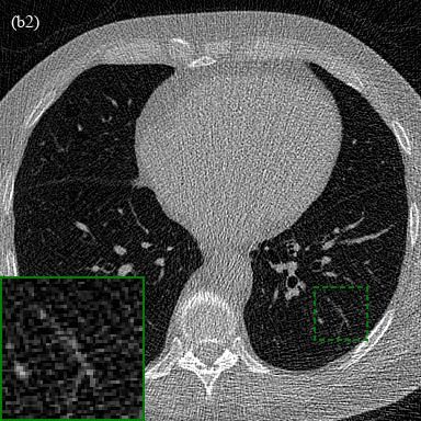
In addition, η ∈ Rk represents the noise in the system [22].
    The number of measurements (k) is reduced to obtain CT images from fewer
numbers of projections. Therefore the forward operator (A) takes the form of
a fat matrix and the sparse CT inverse problem occurs with the formation of a
non-invertible forward operator. The projections used in sparse CT problems
have a high signal-to-noise ratio (SNR) value, but the low number of projections
makes inverse operation an ill-posed problem. Another way to reduce the dose
is to decrease the signal power by reducing tube current and peak voltage while
the number of projections is constant. Any decrease in the signal power, in other
words, lower SNR value, is mathematically modeled by increasing the variance
of the η in (1) and noisy sinograms are obtained. Despite a sufficient number
of observations being obtained, each observation has a low SNR value.
    The lower frequencies are sampled far more than higher frequencies when a
Radon transform is applied to a CT image. Therefore, the traditional methods
use inverse Radon transform to solve the low-dose CT problem by first perform-
ing a filtering process. Thus, a low-frequency dominant image is reconstructed
after filtering. The FBP method applies filters such as Ramp, Hann, Hamming
to the sinogram before doing the inverse Radon transform [23].
    Iterative and DL-based solutions obtain the measurement results with (1)
and calculate the error between measurement and ground truth CT image. The
optimization problem of an image to image reconstruction method can be de-
fined as:

                          ŵ = argmin kfw (X) − Y k2                         (2)
                                  w

    where X and Y represent the sparse or noisy CT image and the ground truth
CT image respectively. In addition, w is the parameters of the model and fw
indicates the nonlinear reconstruction functions such as iterative and DL-based
solutions [15]. The function whose parameters minimize (2) is considered as the
solution.

3    Proposed Method
The success of 2D deep learning-based solutions such as FBP-ConvNet [9], RED-
CNN [12], Learned PD [14] and iRadonMAP [11] for inverse CT problems has
been demonstrated in the literature. However, it is impossible to detect and
reconstruct inter-slice detail losses resulting from sparse or noisy views by a
2D network. On the other hand, these details can be recaptured when the
correlations between the slices are taken into account. Therefore, it is possible
to optimize a reconstruction based on the 3D surface features rather than 2D
edge features. Based on this insight, we propose a deep learning-based solution
for inverse CT problems called 3D U-NetR which utilizes 3D convolutions and
U-Net Architecture. 3D U-NetR operates by mapping initially reconstructed
sinograms with FBP to the ground truth volumetric images. The proposed

                                       4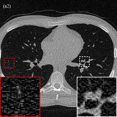
Figure 1: Proposed working schema with 3D U-NetR. τ −1 represents FBP recon-
struction of sparse and noisy sinogram and F denotes image to image mapping
by the proposed 3D U-NetR.

reconstruction process is not limited only to CT images and can be applied to
any 3D imaging modality.
    Firstly, spatial domain forms of the sparse or noisy sinograms are recon-
structed with the inverse operator which can be defined as:

                                  X = τ −1 (x)                               (3)
   where x represents the sparse or noisy sinogram of the image and X repre-
sents the volumetric low-dose CT image. In addition, τ −1 is the inverse operator
and for our case, it is the FBP operator. Low-dose CT images are mapped to
ground truth images with minimum error using the 3D U-NetR architecture.
This can be expressed as:

                                   Ŷ = f (X)                                (4)
    where Ŷ represents the volumetric reconstructed CT image and f is the
trained neural network which is 3D U-NetR. The working principle of the pro-
posed reconstruction method is given in Fig. 1.

3.1    Network Architecture
Based on the success of the 2D FBP-ConvNet [9] architecture and the 3D U-Net
used for segmentation [8], a U-Net like network is built with 3D CNNs. Fig. 2
describes the 3D U-NetR architecture. The network is a modified U-Net with 4
depths which can be inspected as analysis and synthesis parts. The analysis part
of the network contains 2 blocks of 3×3×3 convolution, batch normalization,
and leaky ReLU in each layer. Two layers in consecutive depths are connected
with 2×2×2 max-pooling with stride 2.
    Starting from the deepest layer, layers are connected with a trilinear inter-
polation process with scale factor 2 and followed by 2 blocks of 3×3×3 convolu-
tion, batch normalization, and leaky ReLU for synthesis. Before the convolution
blocks, channels are concatenated with the feature maps from the skip connec-
tions of the corresponding analysis layer. Skip connections are used to solve

                                       5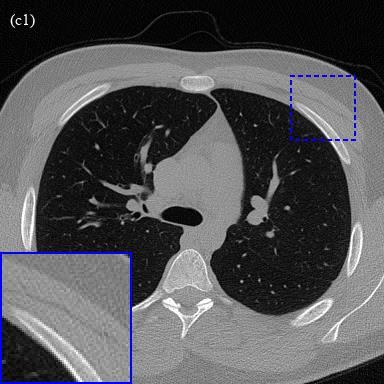
Figure 2: Network Architecture of 3D U-NetR.

the vanishing gradients problem and carry the high-resolution features. On the
other hand, trilinear interpolation is chosen as a simple 3D interpolation method.
Finally, all channel outputs are summed by a 1×1×1 convolution block into 1
channel image and the result is added to the input with shortcut connection.
     Overall, the 3D U-NetR architecture contains 5,909,459 parameters which
are three times of the 2D structure. The number of layers and filters are kept
the same in both networks for a fair comparison which naturally results in an
inequality of number of parameters. Due to high number of parameters and
memory limitations, the number of filters started from 16 in the first layer and
continued to double in each layer up to the deepest one. The number of filters
used in the deepest layer thus became 256. In the synthesis part, the number of
filters in each layer starting from the deepest layer to the output layer decreases
by half in the same manner.
     The skip connections contain 1 block of 1×1×1 convolution, batch normal-
ization, and leaky ReLU rather than shortcut connection to be able to tune the
number of residually connected channels. In addition, a shortcut connection is
connected from the input to the output since the main purpose is to reduce the
noise in the FBP images. The random noise modeling of the network is provided
with the shortcut connection.

                                        6
4       Experimental Setup
4.1     Dataset Preparation
Two datasets are used for the experimentation of the proposed method. Because
of the nature of the CT modality and the network architecture, 3D datasets are
prepared rather than shuffled 2D CT image slices. Firstly, synthetic data which
is a 3D version of the 2D ellipses dataset of Deep Inversion Library (DIVαl) is
prepared [24]. For human CT experiments, a chest dataset acquired from Mayo
Clinic for the AAPM Low Dose CT Grand Challenge is used as the real CT
dataset [25].

4.1.1    Synthetic Data
The previously used ellipses dataset in the literature [9, 14] which contains
randomly generated ellipses is modified to create random ellipsoids in a 3D
space. In the ellipses dataset, the number of ellipses in each image slice is
selected from a Poisson distribution with an expected value of 40 and limited to
70. For our ellipsoid dataset, the number of ellipsoids in each volume is selected
from a Poisson distribution with an expected value of 114 and limited to 200.
Later, each volume is normalized by setting all the negative values to zero and
dividing them to the maximum value of the volume. Finally, all the volumes
are masked with a cylindrical mask along the slice axis in order to be similar to
CT images.
    Parallel beams with 60 views and 182 detectors are chosen as projection
geometry. A sparse view sinogram of each volumetric image slice is obtained
with the forward operator. In addition, additive white Gaussian noise (AWGN)
has been applied to the sinograms with 35 dB SNR. Instead of using a signal-
dependent noise such as the Poisson distribution, the Gaussian distribution is
used to keep the synthetic data simple. The sinograms are reconstructed with
a 2D FBP with Hann filter which has 0.8 frequency scaling for each volumetric
image slice. 2D FBP is chosen instead of 3D FBP operation to prevent the
reconstruction of an extra ellipsoid due to the artifacts in the third dimension.
    220 different volumetric images are generated where each image has 128
slices of 128×128 pixel images. Total volumes are separated as 192 training, 8
validation, and 20 test volumes.

4.1.2    Real Chest CT Data
The real chest CT dataset from Mayo Clinic consists of full-dose and 1/10 of
the normal dose (low-dose) CT image pairs. The 1/10 of the normal dose data
are noisy and have full-view images as there is no reduction in the number
of projections. The low-dose images are created using a realistic and scanner
specific noise insertion model based on Poisson distribution, and inverse square
relation between noise and dose is used to calculate the dose level [26]. Since
2 patients had an unequal number of low-dose and full-dose images, they are
excluded from the dataset, which is containing 50 patients in total. 11 patients

                                        7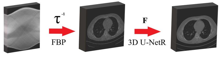
are excluded to decrease the variance of pixel spacing values since convolution
operation is naturally not zoom resistant [27] and different pixel spacing values
have the risk of adversely affecting the training. At the point where the artifact
is present in the CT images, the pixel values of the image become high, which
disrupts the general structure. For this reason, we excluded 9 patients as they
contained artifacts. On the other hand, slices are evenly spaced for every patient
with a 1.5 mm slice thickness.
    Originally, selected patients have 340 ± 18 slices but only the middle 256
slices are used to focus on the middle part of the volumetric image where the
main medical information exists. As Luschner et. al. have mentioned, the
real CT data contain circular reconstructions, and the data must be cropped
at a square inside this circle to prevent value jumps at the circle’s boundaries
[28]. Accordingly, we focused the middle 384×384 pixels of each slice where
there were 512×512 pixels in the original one. Consequently, a dataset of 28
patients with (0.735 ± 0.036)2 mm2 pixel spacing, 1.5 mm slice thickness, and
384×384×256 voxels is prepared.
    Total 28 patients are separated into 25 training and 3 test volumes. In addi-
tion, the volumetric images which are 384×384×256 voxels are divided into 18
volumetric patches with the size of 128×128×128 voxels because of the memory
limitations.

4.2    Training Strategy
The Tesla T4 graphic processing unit (GPU) with 16 GB memory and GeForce
RTX 2080 Ti with 11 GB memory are used during the trainings. Tesla T4
GPU is used in the training with ellipsoids dataset because of the high memory
capacity, and GeForce RTX 2080 Ti is preferred in the training with real chest
CT dataset due to high processing power. L1 norm is utilized for optimization
since it shows better performance in image denoising problems compared to
L2 norm [29]. The error minimization between the reconstructed image and
ground truth image can be achieved with different algorithms. ADAM optimizer
is preferred for this work. The 3D U-NetR architecture is implemented with
PyTorch toolbox [30]. A batch consists of 128×128×128 volumetric images
in 3D U-NetR training. Therefore, when the batch size is higher than 4, the
memory becomes insufficient for both GPUs and the batch size is selected as
4 for the ellipsoids dataset and 3 for the real chest CT dataset for 3D U-NetR
training. 0.001 is chosen as the learning rate and the coefficients to be used for
finding the mean of the gradients and its square are selected as 0.9 and 0.999 by
default. The 3D U-NetR architecture is trained with ellipsoids for 745 epochs,
then the real chest CT for 1108 epochs. The training continues until the change
in loss values become negligible. Training of ellipsoids and real chest CT images
take approximately 62 hours and 166.2 hours, respectively.
    The 2D U-Net architecture is also trained with the slices of the same datasets
in order to show the contribution of the third dimension. PyTorch, Tesla T4
and GeForce RTX 2080 Ti GPUs, L1 norm loss function, and ADAM optimizer
are used as in the 3D U-NetR training. In addition, optimizer parameters

                                        8
such as learning rate, gradient coefficients are kept the same, only batch size
is changed. A batch consists of slices that have a 128×128 size and are taken
from the volumetric images in 2D U-Net training. The batch size is selected
as 384 for the ellipsoids dataset and 256 for the real chest CT dataset. The
2D U-Net is trained along 763 epochs with ellipsoids and 1742 epochs with real
chest CT. Training with the ellipsoids dataset and real chest CT dataset took
approximately 20.5 hours and 56 hours, respectively.

5     Results
Commonly used quantitative metrics are selected such as peak signal-to-noise
ratio (PSNR) and structural similarity (SSIM) to see the quantitative perfor-
mance of 3D U-NetR. The root mean squared error (RMSE) represents L2 error
and is used when calculating PSNR [31]. The definition of the RMSE is given
as follows:
                                   sX
                         RM SE =         kŷi − yi k2                     (5)
                                            i

   where ŷ and y represent the vector forms of the reconstructed and ground
truth image, respectively. In addition, sub-index i denotes each pixel. Similarly,
PSNR can be defined as:
                                             M AXi
                            P SN R = 20 log                               (6)
                                            RM SE
    M AXi is the maximum value of the image which is 255 for 8-bit images.
Even though PSNR is commonly used for image quality assessment, it only
calculates pixel-wise cumulative error and does not represent how similar the
images are. Therefore, the SSIM is used as a second image quality metric to
evaluate the similarity of luminance, contrast, and structure [32].

                                    (2µx µy + c1 )(2σxy + c2 )
                 SSIM (x, y) =                                                (7)
                                 (µ2x + µ2y + σ1 )(σx2 + σy2 + c2 )
   where µx and µy represent the average of reconstructed and ground truth
images, respectively. σx2 and σy2 indicate the variance of reconstructed and
ground truth images, respectively. In addition, σxy is the covariance of the
reconstructed and ground truth image. c1 and c2 constants are calculated based
on the dynamic range of images and they are 2.55 and 7.65 correspondingly for
8-bit images.

5.1    Synthetic Data Reconstruction Results
The performance of 3D U-NetR is examined with the synthetic dataset in this
section. The reconstructed images with the FBP, 2D U-Net, and 3D U-NetR are
given in Fig. 3. As can be seen from the results, some details lost in FBP images

                                        9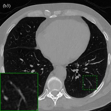
Figure 3: 2 different synthetic image reconstruction examples. Each row denoted
as (a) and (b) represents a different ellipsoid image. Columns (1-4) indicate
ground truth, FBP, 2D U-Net, and 3D U-NetR reconstructions, respectively.

cannot be recovered with 2D U-Net, but with 3D U-NetR. For example, the red
zoom window in Fig. 3 (a1-a4) has a white line-like feature which is missing in
2D U-Net output, but captured by 3D U-NetR. Since 2D U-Net is using only
single slice FBP output, some details lost in FBP cannot be recovered in 2D
U-Net output. Moreover, it has been observed that the 3D U-NetR reconstructs
elliptical edges more smoothly. For instance, when the white zoom windowed
parts in Fig. 3 (a1-a4) are compared, it is observed that the edge of darker ellipse
is not preserved in 2D U-Net output while it is recovered more accurately by
3D U-NetR. PSNR and SSIM metric values of test data are given in Table 1
to show the quantitative performance of the 3D U-NetR. Overall, 3D U-NetR
shows slightly higher mean quantitative performance and has a lower standard
deviation than 2D U-Net which shows the stability of the 3D U-NetR.

5.2    Real Chest CT Data Reconstruction Results
Forward propagation of the real chest CT data is done differently from the el-
lipsoids due to the image size. Even though medical images are patched for
training because of GPU limitations, bigger portions of data can be used as a
whole in forward propagation thanks to the higher memory capacity of the CPU
and RAM. The first thing to note here is the receptive field of network archi-
tecture. 3D U-NetR is a deep and complex network that has a receptive field
of 140×140×140 voxels. In terms of slices, every slice in forward propagation
is affected by the adjacent 70 slices in both directions. Therefore, doing the
reconstruction of each patch separately is highly erroneous. Thus, it is decided
to separately process each patient’s first and last 192 slices and then paste back

                                        10
Phantom No SSIM of FBP SSIM of 2D U-Net SSIM of 3D U-NetR
Phantom 1 72.73±3.12 97.85±0.85 97.81±0.71
Phantom 2 69.83±3.31 98.06±0.50 98.01±0.47
Phantom 3 73.87±2.37 97.44±1.20 97.48±1.03
Phantom 4 71.71±2.48 97.52±0.96 97.56±0.80
Phantom 5 72.22±3.71 97.46±1.36 97.47±1.19
Phantom 6 75.06±3.33 97.52±0.74 97.50±0.67
Phantom 7 73.17±2.81 97.03±1.29 97.07±1.06
Phantom 8 74.84±2.60 97.52±0.86 97.48±0.73
Phantom 9 71.36±3.68 97.20±1.38 97.22±1.18
Phantom 10 73.50±2.63 97.64±1.20 97.74±0.98
Phantom 11 71.81±2.57 96.32±1.45 96.61±1.11
Phantom 12 73.24±3.39 97.04±1.12 97.17±0.94
Phantom 13 73.77±2.66 97.25±1.06 97.37±0.81
Phantom 14 72.95±2.86 97.12±1.35 97.22±1.12
Phantom 15 76.30±3.35 97.80±0.61 97.69±0.64
Phantom 16 75.87±3.37 97.02±0.75 97.05±0.62
Phantom 17 73.56±3.75 97.80±0.68 97.83±0.65
Phantom 18 70.59±3.05 96.89±1.41 97.11±1.09
Phantom 19 74.07±3.42 96.64±1.11 96.86±0.86
Phantom 20 73.30±2.97 97.01±1.16 97.11±0.90
Average 73.19±3.07 97.31±1.05 97.37±0.88
Phantom No PSNR of FBP PSNR of 2D U-Net PSNR of 3D U-NetR
Phantom 1 25.07±1.09 34.02±1.58 33.99±1.32
Phantom 2 25.05±1.38 34.43±1.52 34.52±1.42
Phantom 3 26.34±1.26 34.64±2.08 34.68±1.81
Phantom 4 25.49±1.44 34.21±2.17 34.29±1.82
Phantom 5 25.20±1.76 34.20±2.75 34.13±2.71
Phantom 6 26.68±1.60 34.71±1.63 34.70±1.57
Phantom 7 25.76±1.37 33.70±2.48 33.71±2.20
Phantom 8 26.28±1.25 34.43±1.64 34.31±1.34
Phantom 9 24.87±1.30 33.50±1.65 33.63±1.72
Phantom 10 27.10±0.99 35.40±2.29 35.53±2.03
Phantom 11 25.20±0.87 32.87±1.81 33.04±1.51
Phantom 12 25.95±1.42 33.48±1.62 33.71±1.54
Phantom 13 25.74±1.22 33.99±1.91 34.06±1.62
Phantom 14 27.13±1.23 34.86±1.83 35.01±1.63
Phantom 15 26.98±1.59 35.42±1.68 35.30±1.69
Phantom 16 26.47±1.36 34.03±1.56 34.07±1.39
Phantom 17 26.50±1.48 35.06±1.56 35.11±1.54
Phantom 18 25.78±1.49 34.01±2.58 34.12±2.22
Phantom 19 27.19±1.17 33.73±1.34 34.04±1.20
Phantom 20 25.98±1.21 33.83±1.74 33.86±1.40
Average 26.04±1.32 34.23±1.87 34.29±1.68
Table 1: Quantitative results of the FBP, 2D U-Net and 3D U-NetR with syn-
thetic images
11Figure 4: 3 different real chest CT image reconstruction examples. Each row
denoted as (a), (b), and (c) indicates a different real chest CT image. Columns
(1-4) represent ground truth, FBP, 2D U-Net, and 3D U-NetR outputs, respec-
tively. The images are displayed using the 0-0.45 normalized window, which
corresponds to [-1024, 820] HU.
the first and last 128 slices for forward propagation. Hereby, an interval of 64
slices starting from the middle is used only as padding for other voxels. Still, it
is 6 slices less than the ideal value but restrictions on resources enable this as
the way to reconstruct with minimum error.
We further investigated the performance of 3D U-NetR, which has been
trained with low and high-dose real chest CT images prepared by the Mayo
Clinic. The ill-posed problem with synthetic data is easier than real chest CT
images since synthetic data contains images with less resolution. The results for
the reconstructed images with the FBP and the forward propagated images with
trained 2D U-Net and 3D U-NetR are provided in Fig. 4. As can be seen from
the figure, 3D U-NetR captures some details that FBP and 2D U-Net cannot
reconstruct. Some details lost in the vessels and bone tissue due to noise in
low-dose images cannot be obtained with FBP and 2D U-Net. For example, the
horizontal vessel in red zoom window in Fig. 4 (a1-a4) is lost when 2D U-Net is
used, but successfully recovered with 3D U-NetR. When the blue zoom window
in Fig. 4 (c1-c4) is examined, it is seen that 3D U-NetR captures a diagonal
line-like detail which is missing in 2D U-Net. Overall, 3D U-NetR recovers
12Patient No SSIM of FBP SSIM of 2D U-Net SSIM of 3D U-NetR
Patient 1 45.33±8.59 80.01±5.69 81.65±5.56
Patient 2 35.33±5.95 69.18±5.93 71.07±5.84
Patient 3 38.86±7.97 74.55±6.27 76.20±6.10
Average 39.84±7.50 74.58±5.96 76.31±5.83
Patient No PSNR of FBP PSNR of 2D U-Net PSNR of 3D U-NetR
Patient 1 23.87±2.04 32.97±1.46 33.82±1.46
Patient 2 20.75±1.58 30.20±1.44 30.84±1.34
Patient 3 22.05±1.58 31.53±1.12 32.21±1.11
Average 22.23±1.74 31.57±1.34 32.29±1.30
Table 2: Quantitative performance of the FBP, 2D U-Net and 3D U-NetR with
Real CT images
the details since it takes into account the correlation between slices. The total
quantitative results of the 3D U-NetR are displayed in Table 2 in terms of
PSNR and SSIM. The quantitative performance of 3D U-NetR is considerable
more than 2D U-Net in every patient for real chest CT data.
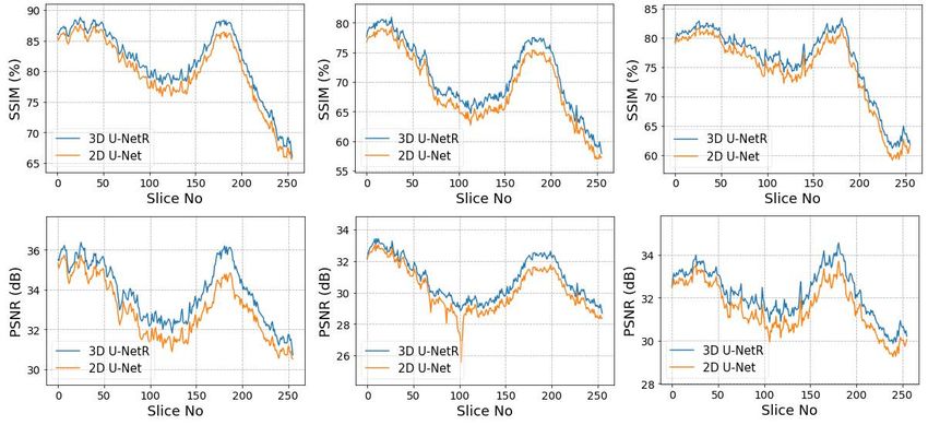
Although looking at the average PSNR and SSIM values of the reconstructed
CT images gives information about performance, it does not does not guarantee
the stability of the networks For this reason, it is also important to examine the
performances based on slices. Fig. 5 shows the SSIM and PSNR values of each
slice of the patients one by one. It is observed that 3D U-NetR’s superiority
in average performance is not due to instant improvements, but generally has
better performance in each slice. In addition, 2D U-Net has a high deviation
at some points, while 3D U-NetR is more stable since it takes into account the
correlation in the third dimension.
Figure 5: PSNR and SSIM values of 2D U-Net (presented with orange line) and
3D U-NetR (presented with blue line) for each slice of 3 test patients whose
average scores are given in Table 2.
136 Discussion and Conclusion
In this paper, 3D U-NetR architecture is proposed for CT image reconstruction,
inspired by 3D networks previously used for image segmentation. The novel
part of 3D U-NetR from other networks that reconstruct CT images in the
literature is 3D U-NetR evaluates the image as 3D data and optimizes filter in
all three dimensions. The details lost in a 2-dimensional slice can be recovered
by examining the third dimension and this has been proven with the prepared
experimental setups.
Two different datasets, including synthetic and real chest CT images, are
used to validate the model. 3D U-NetR has a difference of 8 dB and 24 percent
in terms of PSNR and SSIM, respectively, to the traditional FBP method, and it
contains much fewer artifacts visually in the synthetic ellipsoids dataset. When
3D U-NetR is compared with 2D U-Net, the quantitative performance of 3D
U-NetR appears to be ahead. In addition, when the images are examined, it is
seen that 3D U-NetR reconstructs the edges of the ellipses better and captures
some small details which are lost in 2D U-Net’s outputs, and this proves that
3D U-NetR is better in synthetic data. The success of 3D U-NetR in sparse
view has been shown with the synthetic dataset since it contains a low number
of projections.
3D U-NetR has the best quantitative performance among the networks
trained with real chest CT images dataset. In addition, it is seen that some
details are lost with 2D U-Net and FBP in real chest CT images, as in synthetic
data images. However, some vessels in the lung and some tissues in the bone are
better recovered with 3D U-NetR. The ability of 3D U-NetR to capture details
in vascular and soft tissue is evidence that low-dose CT can become commer-
cially widespread and 3D networks can be used for denoising along with the
increasing hardware specs.
The noise model of the synthetic dataset is chosen as Gaussian, which does
not mimic perfectly the low-dose CT noise unlike Poisson distribution, for the
simplicity in sparse view case. However, Mayo Clinic dataset contains the Pois-
son noise distribution along with the electronic noise. In addition, the biggest
problem in the real chest CT dataset is that the images labeled as ground truth
contain a certain amount of noise. The noise in ground truth images causes
PSNR and SSIM metrics to be lower than synthetic data. Although PSNR and
SSIM metrics are frequently used in the literature, they are not sufficient to
emphasize the visual detail differences and quantitative performance in terms
of PSNR and SSIM is not fully reliable in medical imaging [33]. Therefore, the
visually captured details are presented along with quantitative performance in
the evaluations.
3D U-NetR gives better results because it takes into account the correlation
in the third dimension, but it also has some disadvantages such as high time
for training, the limited number of filters, and patched training due to memory
limitations.
First of all, since the convolution blocks in the network are 3-dimensional,
the number of parameters is approximately three times that of 2-dimensional
14networks. The high number of parameters causes the network’s loss curve to
settle with more iterations and require more time for training. Different experi-
mental setups such as residual connection, the filter number, activation function
selection, and different configurations of the dataset could not be prepared be-
cause the network requires a high time for training.
Secondly, increasing the number of filters might have an exponential impact
on performance compared to 2D convolutions. Although the highest number
of possible filters is already preferred in experimental setups, the maximum
number of available filters in 3D U-NetR is fewer than 2D U-Net due to memory
limitations.
Finally, the high memory consumption of 3D U-NetR obstructs the back-
propagation of high-resolution human CT images. Hence, the real chest CT
dataset is used by splitting 3D images into patches. Even though the patch-
ing operation eliminates the memory limitation, the intersection points of the
patches show deformation on direct reconstruction. Thus, patches are designed
to have common intersection parts which are equivalent to the half of receptive
field of the network as explained in Section 5.2. Overall, the patched training,
which is needed because of stricter memory limitations of 3D U-NetR, causes
higher calculation time.
The proposed method gives better results with both real and synthetic data
compared to its 2-dimensional configuration. Since the scope of the study is the
exploration of third-dimensional information with a 3D network, other state of
the art networks, such as generative adversarial networks (GAN) and encoder-
decoder architecture, are not used in the comparison.
In addition, 3D U-NetR can be applied to different experimental setups
containing CT images and different imaging modalities. 3D convolutions can
also be used with projection data for improvement in spatial domain. Our future
studies will address these topics.
References
[1] L. A. Shepp and B. F. Logan, “The fourier reconstruction of a head sec-
tion,” IEEE Transactions on Nuclear Science, vol. 21, no. 3, pp. 21–43,
1974.
[2] A. H. Andersen and A. C. Kak, “Simultaneous algebraic reconstruction
technique (sart): a superior implementation of the art algorithm,” Ultra-
sonic imaging, vol. 6, no. 1, pp. 81–94, 1984.
[3] R. Gordon, R. Bender, and G. T. Herman, “Algebraic reconstruction tech-
niques (art) for three-dimensional electron microscopy and x-ray photogra-
phy,” Journal of theoretical Biology, vol. 29, no. 3, pp. 471–481, 1970.
[4] E. Y. Sidky and X. Pan, “Image reconstruction in circular cone-beam com-
puted tomography by constrained, total-variation minimization,” Physics
in Medicine & Biology, vol. 53, no. 17, p. 4777, 2008.
15[5] J. Wang, T. Li, H. Lu, and Z. Liang, “Penalized weighted least-squares
approach to sinogram noise reduction and image reconstruction for low-
dose x-ray computed tomography,” IEEE transactions on medical imaging,
vol. 25, no. 10, pp. 1272–1283, 2006.
[6] D. Kumar, A. Wong, and D. A. Clausi, “Lung nodule classification using
deep features in ct images,” in 2015 12th Conference on Computer and
Robot Vision. IEEE, 2015, pp. 133–138.
[7] B. A. Skourt, A. El Hassani, and A. Majda, “Lung ct image segmentation
using deep neural networks,” Procedia Computer Science, vol. 127, pp. 109–
113, 2018.
[8] Ö. Çiçek, A. Abdulkadir, S. S. Lienkamp, T. Brox, and O. Ronneberger, “3d
u-net: learning dense volumetric segmentation from sparse annotation,”
in International conference on medical image computing and computer-
assisted intervention. Springer, 2016, pp. 424–432.
[9] K. H. Jin, M. T. McCann, E. Froustey, and M. Unser, “Deep convolutional
neural network for inverse problems in imaging,” IEEE Transactions on
Image Processing, vol. 26, no. 9, pp. 4509–4522, 2017.
[10] B. Zhu, J. Z. Liu, S. F. Cauley, B. R. Rosen, and M. S. Rosen, “Image
reconstruction by domain-transform manifold learning,” Nature, vol. 555,
no. 7697, pp. 487–492, 2018.
[11] J. He, Y. Wang, and J. Ma, “Radon inversion via deep learning,” IEEE
Transactions on Medical Imaging, vol. 39, no. 6, pp. 2076–2087, 2020.
[12] H. Chen, Y. Zhang, M. K. Kalra, F. Lin, Y. Chen, P. Liao, J. Zhou, and
G. Wang, “Low-dose ct with a residual encoder-decoder convolutional neu-
ral network,” IEEE transactions on medical imaging, vol. 36, no. 12, pp.
2524–2535, 2017.
[13] H. Xie, H. Shan, and G. Wang, “Deep encoder-decoder adversarial recon-
struction (dear) network for 3d ct from few-view data,” Bioengineering,
vol. 6, no. 4, p. 111, 2019.
[14] J. Adler and O. Öktem, “Learned primal-dual reconstruction,” IEEE trans-
actions on medical imaging, vol. 37, no. 6, pp. 1322–1332, 2018.
[15] H. Chen, Y. Zhang, W. Zhang, P. Liao, K. Li, J. Zhou, and G. Wang,
“Low-dose ct denoising with convolutional neural network,” in 2017 IEEE
14th International Symposium on Biomedical Imaging (ISBI 2017), 2017,
pp. 143–146.
[16] V. Lempitsky, A. Vedaldi, and D. Ulyanov, “Deep image prior,” in 2018
IEEE/CVF Conference on Computer Vision and Pattern Recognition.
IEEE, 2018, pp. 9446–9454.
16[17] D. O. Baguer, J. Leuschner, and M. Schmidt, “Computed tomography re-
construction using deep image prior and learned reconstruction methods,”
Inverse Problems, vol. 36, no. 9, p. 094004, 2020.
[18] L. Gondara, “Medical image denoising using convolutional denoising au-
toencoders,” in 2016 IEEE 16th International Conference on Data Mining
Workshops (ICDMW), 2016, pp. 241–246.
[19] O. Ronneberger, P. Fischer, and T. Brox, “U-net: Convolutional networks
for biomedical image segmentation,” in International Conference on Medi-
cal image computing and computer-assisted intervention. Springer, 2015,
pp. 234–241.
[20] S. Liu, D. Xu, S. K. Zhou, O. Pauly, S. Grbic, T. Mertelmeier, J. Wick-
lein, A. Jerebko, W. Cai, and D. Comaniciu, “3d anisotropic hybrid net-
work: Transferring convolutional features from 2d images to 3d anisotropic
volumes,” in International Conference on Medical Image Computing and
Computer-Assisted Intervention. Springer, 2018, pp. 851–858.
[21] H. Shan, Y. Zhang, Q. Yang, U. Kruger, M. K. Kalra, L. Sun, W. Cong,
and G. Wang, “3-d convolutional encoder-decoder network for low-dose ct
via transfer learning from a 2-d trained network,” IEEE transactions on
medical imaging, vol. 37, no. 6, pp. 1522–1534, 2018.
[22] M. O. Unal, M. Ertas, and I. Yildirim, “An unsupervised reconstruction
method for low-dose ct using deep generative regularization prior,” 2020.
[23] X. Pan, E. Y. Sidky, and M. Vannier, “Why do commercial CT scanners
still employ traditional, filtered back-projection for image reconstruction?”
Inverse Problems, vol. 25, no. 12, p. 123009, dec 2009. [Online]. Available:
https://doi.org/10.1088/0266-5611/25/12/123009
[24] J. Leuschner, M. Schmidt, and D. Erzmann, “Deep inversion validation
library,” https://github.com/jleuschn/dival, 2019.
[25] C. McCollough, B. Chen, D. Holmes, X. Duan, Z. Yu, L. Xu, S. Leng,
and J. Fletcher, “Low dose ct image and projection data [data set],” The
Cancer Imaging Archive, 2020.
[26] T. R. Moen, B. Chen, D. R. Holmes III, X. Duan, Z. Yu, L. Yu, S. Leng,
J. G. Fletcher, and C. H. McCollough, “Low-dose ct image and projection
dataset,” Medical physics, vol. 48, no. 2, pp. 902–911, 2021.
[27] I. Goodfellow, Y. Bengio, and A. Courville, Deep Learning. MIT Press,
2016, http://www.deeplearningbook.org.
[28] J. Leuschner, M. Schmidt, D. O. Baguer, and P. Maaß, “The lodopab-ct
dataset: A benchmark dataset for low-dose ct reconstruction methods,”
arXiv preprint arXiv:1910.01113, 2019.
17[29] H. Zhao, O. Gallo, I. Frosio, and J. Kautz, “Loss functions for image
restoration with neural networks,” IEEE Transactions on computational
imaging, vol. 3, no. 1, pp. 47–57, 2016.
[30] A. Paszke, S. Gross, F. Massa, A. Lerer, J. Bradbury, G. Chanan,
T. Killeen, Z. Lin, N. Gimelshein, L. Antiga, A. Desmaison, A. Kopf,
E. Yang, Z. DeVito, M. Raison, A. Tejani, S. Chilamkurthy, B. Steiner,
L. Fang, J. Bai, and S. Chintala, “Pytorch: An imperative style,
high-performance deep learning library,” in Advances in Neural
Information Processing Systems 32. Curran Associates, Inc., 2019,
pp. 8024–8035. [Online]. Available: http://papers.neurips.cc/paper/
9015-pytorch-an-imperative-style-high-performance-deep-learning-library.
pdf
[31] W. Yuanji, L. Jianhua, L. Yi, F. Yao, and J. Qinzhong, “Image quality
evaluation based on image weighted separating block peak signal to noise
ratio,” in International Conference on Neural Networks and Signal Pro-
cessing, 2003. Proceedings of the 2003, vol. 2. IEEE, 2003, pp. 994–997.
[32] Z. Wang, E. P. Simoncelli, and A. C. Bovik, “Multiscale structural simi-
larity for image quality assessment,” in The Thrity-Seventh Asilomar Con-
ference on Signals, Systems & Computers, 2003, vol. 2. Ieee, 2003, pp.
1398–1402.
[33] J.-F. Pambrun and R. Noumeir, “Limitations of the ssim quality metric in
the context of diagnostic imaging,” in 2015 IEEE International Conference
on Image Processing (ICIP). IEEE, 2015, pp. 2960–2963.
18You can also read