A consistent and comprehensive computational approach for general Fluid-Structure-Contact Interaction problems
←
→
Page content transcription
If your browser does not render page correctly, please read the page content below

A consistent and comprehensive computational approach for
                                                 general Fluid-Structure-Contact Interaction problems

                                                                 Christoph Ager∗ , Alexander Seitz, Wolfgang A. Wall
                                                                 Institute for Computational Mechanics , Technical University of Munich,
                                                                               Boltzmannstr. 15, 85747 Garching b. München
arXiv:1905.09744v1 [cs.CE] 23 May 2019

                                                                                              SUMMARY
                                         We present a consistent approach that allows to solve challenging general nonlinear fluid-structure-contact
                                         interaction (FSCI) problems. The underlying continuous formulation includes both ”no-slip” fluid-structure
                                         interaction as well as frictionless contact between multiple elastic bodies. The respective interface conditions
                                         in normal and tangential orientation and especially the role of the fluid stress within the region of closed
                                         contact are discussed for the general problem of FSCI. To ensure continuity of the tangential constraints
                                         from no-slip to frictionless contact, a transition is enabled by using the general Navier condition with
                                         varying slip length. Moreover, the fluid stress in the contact zone is obtained by an extension approach
                                         as it plays a crucial role for the lift-off behavior of contacting bodies. With the given continuity of the
                                         spatially continuous formulation, continuity of the discrete problem (which is essential for the convergence
                                         of Newton’s method) is reached naturally. As topological changes of the fluid domain are an inherent
                                         challenge in FSCI configurations, a non-interface fitted Cut Finite Element Method (CutFEM) is applied to
                                         discretize the fluid domain. All interface conditions, that is the “no-slip” FSI, the general Navier condition,
                                         and frictionless contact are incorporated using Nitsche based methods, thus retaining the continuity and
                                         consistency of the model. To account for the strong interaction between the fluid and solid discretization,
                                         the overall coupled discrete system is solved monolithically. Numerical examples of varying complexity are
                                         presented to corroborate the developments. In a first example, the fundamental properties of the presented
                                         formulation such as the contacting and lift-off behavior, the mass conservation, and the influence of the slip
                                         length for the general Navier interface condition are analyzed. Beyond that, two more general examples
                                         demonstrate challenging aspects such as topological changes of the fluid domain, large contacting areas, and
                                         underline the general applicability of the presented method.

                                         KEY WORDS: Fluid-struture interaction; Contact mechanics; CutFEM; Nitsche’s method; general
                                                    Navier condition

                                                                                        1. INTRODUCTION

                                         The development of a consistent and comprehensive computational approach that allows to
                                         investigate fluid-structure interaction (FSI) including contact† of submersed elastic bodies is the
                                         focus of this contribution. Applications, ranging e.g. from the dynamic behavior of biological
                                         or mechanical valves to hydrodynamic bearings and tire/wet road contact, often require reliable
                                         formulations to solve the fluid-structure-contact interaction (FSCI) problem. As motivated by these
                                         examples, examinations will be carried out at system scale, at which the relevant physics can be well

                                         ∗
                                           Correspondence to: Christoph Ager, Institute for Computational Mechanics, Technical University of Munich,
                                         Boltzmannstraße 15, D-85747 Garching, Germany. E-mail: ager@lnm.mw.tum.de
                                         †
                                           The terms “contact”, “solid-solid interaction”, or “solid-solid contact” are exclusively used for the interaction of two
                                         solid bodies/domains in this work. Other phase boundaries, which are sometimes also referred to as “contact”, are not
                                         considered in this contribution.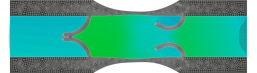
2                                             C. AGER ET AL.

                            fluid-structure interaction ⇐⇒ solid-solid contact
       1                                2                   1                              2
                                                    3
                                                                                            3
                   2                                                   2

                                    2               3                                     2
                                                                                              3

               2                                                        2

Figure 1. Detailed view of solid-solid contact with surrounding fluid in two only slightly different states
of contact (top). Visualization of the acting force on the solid boundary by arrows. Blue arrows indicate
the traction due to the fluid-structure interaction and black arrows indicate the traction due to solid-solid
contact (bottom). The following symbols are used: 1 , fluid domain resolved by macroscopic model; 2 ,
                                  solid domain; 3 , solid-solid contact zone.

represented by means of the continuum mechanics theory. Challenges for corresponding numerical
methods, among others, include the handling of the occurring topological changes in the fluid
domain, the numerical stability of the formulation, the representation of a physical solution close
to the interface, and the transition between fluid-structure interaction and contact. For a limited
range of problems, the explicit numerical treatment of contact can be avoided by smartly chosen
boundary conditions in the setup of the numerical problem and then solved in existing classical FSI
frameworks. These strategies of circumventing the general problem of FSCI, which causes quite a
limitation with respect to many applications, are not the focus of this work.
   The physical processes involved in contacting bodies submersed in fluid modeled by continuum
mechanics theory did not get sufficient attention in previous developments to solve FSCI
numerically. FSCI on a macroscopic length scale is characterized by topological changes of the
fluid domain. On this scale it is important how potential fluid dynamics effects between bodies
in the zone of contacting solid interfaces are modeled. Thus, we first provide a comprehensible
clarification of the involved phenomena and discuss resulting implications for the physical modeling
for a macroscopic description of FSCI. The purely geometric classical contact condition that solid
bodies are not allowed to penetrate each other directly applies also in the presence of fluid. In
contrast to that, the usual condition from dry contact that no tensile forces can be transmitted
between the contacting bodies requires deeper insight into the contacting process. In Figure 1
(top), two configurations for contact of two elastic bodies submersed in fluid are shown. Both
configurations only differ by a slightly different vertical position of the upper solid body, i.e.
already small displacements allow to transfer one into the other. For a continuous formulation, small
changes in the position of solid bodies should result only in small changes of the interface traction.
This aspect is highlighted in Figure 1 (bottom), where the fluid is replaced by the force acting
on the respective solid boundaries. Therein, the FSI traction (indicated by blue arrows) transfers
into the contact traction (indicated by black arrows) and vice versa. For a continuous problem, the
magnitude of the acting traction is not allowed to jump at the transition between interface regions
with these two types of condition. To ensure that, we define the FSI traction on the entire interface.
This applies especially for the solid-solid contact zone which is located between the two contacting
bodies (see Figure 1, interface zone 3 ), even if the enclosed fluid domain is not represented by the
macroscopic fluid model. This enables a continuous transition from the contact to the FSI traction
which otherwise would not be possible. It is worth mentioning that this is not unphysical or only a
“numerical ’trick”, as in reality fluid will still remain at this interface but would only be visible on
a smaller length scale. The no-adhesive force condition of classical contact mechanics can thereby
be reformulated based on the difference between contact and fluid traction.
   As a result of this setup increasing the fluid pressure can lift-off two contacting bodies not only
in the physical world but also in the numerical model. This effect demonstrates the importance of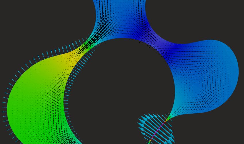
A CONSISTENT AND COMPREHENSIVE APPROACH FOR FSCI                                3

a defined fluid stress state at every point in the contact zone. Depending on different criteria, fluid
models of variable complexity and accuracy on the reduced dimensional manifold of the contact
zone can be considered. These criteria include the microstructure of the contacting surfaces (smooth
vs. rough), the quantities/processes of interest (e.g. leakage of a sealing), and the macroscopic
problem configuration (closed vs. open fluid domain). As this work intends to provide a general
FSCI framework, a simple extension based approach to model the fluid in the contact zone is applied
herein. The general framework then allows to include also various types of alternative and more
sophisticated fluid models in the contact zone in the future. For a model with greater physical depth,
the reader is e.g. referred to [1], where a homogenized poroelastic layer formulation is applied to
model the fluid flow through contacting rough surfaces.
   When looking at the available literature one can note that a large portion of literature on
FSCI formulations is either interested in the analysis of heart valves [2–11] and only a smaller
set in solving a more general problem setup of FSCI [1, 12–16]. However, while most of those
formulations work well for certain problem setups, they suffer from some restrictions preventing
their application to more general complex problem classes. In the following we try to give a brief
overview on existing formulations but will not describe the different approaches in detail but rather
point to certain features and especially to assumptions or restrictions.
   In [7, 8] contact in surrounding fluid does not need to be considered due to the chosen problem
setup with geometrically separated contact and fluid-structure interfaces. A penetration of the solid
bodies is accepted in [2] since contact is not treated explicitly. In [6], contact is included, but
in the presented computations only the valve opening phase without significant influence of the
contact formulation is analyzed. In [14], no explicit contact formulation is considered and a minimal
distance of one mesh cell still remains between two flaps. Using reduced modeling with included
contact of the heart valve, [10] avoids the requirement for a general FSCI formulation. In [1], a very
general FSCI formulation for contact of rough surfaces is presented, where the interface is modeled
via a homogenized poroelastic layer. Such a formulation is very powerful and also well motivated
by the involved physical phenomena but it is also more complex and not always needed. In such
frequent cases the approach presented in this paper will be a better alternative.
   Explicit treatment of the contact is considered in [1,3–5,13] by Lagrange multiplier based contact
methods, in [6, 9, 12, 15] by methods based on penalty contact contributions, and in [11] by an
approach based on enforcement of equal structural velocity. Interface fitted computational meshes
for discretization of the fluid domain are enabled by approaches that require to enforce a non-
vanishing fluid gap between approaching bodies and therefore avoid topological changes in the
fluid domain preventing degenerated elements [12, 15]. Approaches enabling the use of a non-
interface fitted discretization, which allow the consideration of “real” contact scenarios and the
resulting topological changes of the fluid domain directly, are applied in [1–6, 9–11, 13, 14]. The
majority of these formulations consider dimensionally reduced structural models (i.e. membranes
and shells) [2–6,9–11], whereas bulky structures (i.e. structures of significant thickness as compared
to the spatial resolution of the computational discretization in the fluid domain) are only considered
in [1, 13, 14, 16]. The restriction to slender bodies of the non-interface fitted approaches is often
related to issues concerning system conditioning and mass conservation errors close to the fluid-
structure interface. This is due to the fact that the discontinuity of the fluid stress between two
sides of a submersed solid typically is not represented by the discrete formulation (see e.g. [9, 10]),
which prevents the analysis of configurations including large pressure jumps. This issue is not a
fundamental limitation for non-interface fitted FSI as shown e.g. in [17, 18] (without contact), but
increases the complexity of such a formulation including the underlying algorithm.
   It is surprising that, except for [1, 16], none of the referenced works includes a substantial
discussion concerning the requirement for the fluid state in the contact zone as elaborated earlier.
Most works include contact just as a constraint additional to the incorporation of FSI conditions,
which is still enforced in closed contact. If such an approach is carried out properly, it can result
in a continuous FSCI formulation. Still, the strategy to recover the fluid state in the contact zone,
which is required to enforce the FSI conditions, remains an open question. For formulations which
circumvent topological changes of the fluid domain [12, 15] this issue does not arise directly, as

4                                            C. AGER ET AL.

there is always a numerically motivated fluid domain in between the contacting bodies. For all other
formulations which support the actual contact of surfaces, the different approaches for the numerical
solution of the fluid problem provide a nonphysical fluid state outside the fluid domain in the contact
zone by default, which builds the basis to incorporate the FSI interface conditions. Depending on the
underlying numerical method and the respective FSCI problem, this can provide, but not necessarily
is, a sufficiently good approximation of the fluid state in the contact zone. We would like to point
out that this fluid state in the contact zone has an essential influence for example to the detaching
behavior of contacting solid bodies, e.g. a high/low fluid pressure supports/prohibits the separation
of two bodies. Another important aspect which should be considered when applying such a strategy
of incorporating contact on top of the FSI conditions is that the FSI traction includes a tangential
component. In contrast to the normal component of the FSI traction, which serves merely as an
offset to normal contact traction, the tangential component directly acts on the contacting surfaces
potentially deteriorating the solution accuracy.
   In this paragraph, we would like to comment briefly on the so called “collision paradox”, which
states that for incompressible, viscous fluid with “no-slip” condition on smooth boundaries, contact
between submersed bodies cannot occur in finite time (see e.g. [19, 20]). This is in contrast to
the observation of contacting solid bodies which is also observed when bodies are submersed
in fluid. A physical explanation for this paradox can be found in the missing consideration of
non-smooth surfaces (analyzed in e.g. [21, 22]) arising from the rough microstructure, or other
effects on the micro scale, not considered in the macroscopic fluid model of the “no-slip” boundary
condition [23]. Nevertheless, even for the computational analysis of physical models where these
effects are not considered, contact still has to be considered. This is a result of the numerical solution
approaches which are always accompanied by approximations of the underlying physical model
when considering general configurations. If there is no explicit contact treatment within the FSI
formulation only fluid forces in the gap keep the bodies apart. But when an artificial collision of
solid bodies occurs, e.g. during an iterative nonlinear solution procedure, there is no separation
force acting as there is no remaining fluid between these bodies. This is shown in [2, 5], where a
penetration of surfaces can be observed as no contact formulation is considered.
   In this contribution, we present a general FSCI formulation considering flows based on the
incompressible Navier-Stokes equations interacting with nonlinear elastic solids that are not
restricted to slender structural bodies. Therein, contact is not considered as a mere additional
constraint on the FSI problem, but focus is rather put on the mutual exclusiveness of fluid-solid
and solid-solid coupling. Thus, the application of fluid forces on the interface in the zone of active
contact, where typically no good representation of the fluid solution is available, is automatically
eliminated. The approach is applied to non-interface fitted discretizations for the fluid domain by
the Cut Finite Element Method (CutFEM), due to its ability to represent sharp discontinuities of
the solution at the interface. This is of essential importance for the discrete representation of the
prevalent discontinuity of the fluid stress between opposite sides of (potentially thin) structural
bodies. Hence, non-physically high gradients arising from a continuous fluid solution representation
can be avoided (see remark in [4, page 1753]). Crucial for a continuous discrete form is the
continuity of the transition from fluid-solid to solid-solid interaction, which is achieved by the use
of Nitsche-based methods for both constraints.
   The CutFEM in general enables the use of non-interface fitted, fixed Eulerian meshes for the fluid
discretization in complex and deforming domains. This method is perfectly suited for handling of
large interface motion and topological changes of the computational domain, typically occurring
for FSCI problems, and therefore is applied here. To enable a determined, continuous transition
from the “no-slip” condition to frictionless contact, a relaxation of the tangential constraint is
proposed, while retaining the mass-balance in normal direction. This is enabled by a flexible
formulation capable of handling the “no-slip” and the “full-slip” limit on the fluid-solid interface.
CutFEM has seen great progress in recent years and meanwhile enjoys a solid mathematical base.
Initial analysis was performed for the Poisson equation [24], extended to the Stokes equation
[25, 26], and finally, including advection, on the Oseen equation [27, 28]. Therein, a so-called
“ghost penalty” stabilization [29] guarantees a well-conditioned formulation for arbitrary interface

A CONSISTENT AND COMPREHENSIVE APPROACH FOR FSCI                                5

positions. Successful applications of the CutFEM on two-phase flow and fluid-structure interaction
are presented in [30–32] and [17, 33, 34], respectively. Therein, the “no-slip” interface condition is
applied weakly by a Nitsche-based method. The basis for the general Navier interface condition
applied in this work was presented for the Poisson equation in [35], extended to the general Navier
boundary condition for the Oseen equation in [36], and applied to enforce the tangential coupling
condition on the interface of an poroelastic solid and a viscous fluid in [1, 37].
   To obtain a continuous transition of the discrete formulation from fluid-structure to contact
interaction, both FSI and the treatment of contact are enforced via Nitsche’s method. A first
application of Nitsche’s method to contact problems was presented in [38]. More recently, the
development of Nitsche-type methods for contact problems gained more attention due to the
mathematical analysis of symmetric and skew-symmetric Nitsche methods provided by [39–41] for
small deformation frictionless and frictional contact problems. In addition, [42] analyzed a penalty-
free variant for the Signiorini-problem. Based on these works, [43] extended Nitsche’s method to
nonlinear elasticity at finite deformation and [44] to nonlinear thermomechanical problems. Most
classical contact formulations employ a so-called slave-master concept introducing an inherent bias
to the formulation by a (user-defined) choice of the slave and master surface. In the context of
Nitsche methods, [43, 45] introduced an unbiased variant. The method proposed in [44] is based on
a harmonic weighting of the contact stress resulting in an almost unbiased approach as the only bias
is introduced by the applied integration rule. In this work, we will extend the method of [44] to a
completely unbiased form by integrating not only on the slave but also on the master surface similar
to so-called two-half-pass algorithms [46]. Finally, the transition between active and inactive contact
has to be balanced carefully with the ambient fluid traction to achieve continuity of the discrete
formulation.
   The resulting formulation is discretized in time by the one-step-θ scheme. Finally, the nonlinear
system of equations is solved for all unknowns, i.e. nodal structural displacements, fluid velocities
and pressures, by a Newton-Raphson based procedure. Due to the strong interaction of all involved
physical domains for the FSCI problem this is done simultaneously, i.e. a monolithic procedure is
applied (see e.g. [47]).
   Recently, [16] presented a Nitsche-based formulation for FSCI similar to the one derived in this
paper. Therein, linear Stokes flow and linear elastic solids based on a fully Eulerian description in
combination with contact to a rigid, straight obstacle at the fluid boundary is analyzed and stability
results for this formulation are shown. In contrast to the extrapolation based strategy proposed in
this contribution, which allows for complete topological changes, two strategies based on a thin
remaining fluid film are presented in [16] to obtain the fluid stress in the contacting zone.
   The paper is organized as follows. In Section 2 the governing equations, comprised of the
structural and fluid mechanics model as well as conditions on the interface in normal an tangential
direction of the FSCI problem, are given. This is followed by a presentation of the discrete
formulation, including all volume and interface contributions, and the solution strategy in Section 3.
Different numerical examples, capable of analyzing different aspects of the formulation, are
presented in Section 4. Finally, in Section 5 a short summary and an outlook are given.

                                  2. GOVERNING EQUATIONS

In this section, we discuss the governing equations and conditions for all physical domains and
interfaces of the FSCI problem. A typical configuration for such a problem is shown in Figure 2.
The domain Ω of the overall FSCI problem includes the fluid domain ΩF and the solid domain
ΩS . The overall coupling interface Γ consists of the fluid-structure interface ΓF S and the active
(closed) contact interface ΓS,c . The different boundaries on the outer boundary ∂ Ω are denoted
by ΓF,D , ΓF,N , ΓS,D , and ΓS,N . In the following, all quantities ∗ , ∗ with additional “zero”-index
∗0 , ∗0 are described in the undeformed reference/material configuration, whereas a missing index
indicates the current configuration (see [48] for details). An additional “hat”-symbol ∗ˆ , ˆ
                                                                                            ∗ indicates
time-dependent prescribed quantities at the boundaries and in the domains. Prescribed quantities at
6                                               C. AGER ET AL.

                                                           ΓFS1
                                    ΩF                        Γ1 = ΓFS1 ∪ ΓS1 ,c
                                                  ΩS1
                                                      ΓS1 ,c
                                                                            ΓF,N
                             ΓF,D                 Γ S2 ,c
                                          Γ2 = ΓFS2 ∪ ΓS2 ,c
                                                            ΩS2
                                           FS2
                                         Γ
                                                 ΓS,D ∪ ΓS,N

Figure 2. Fluid-structure-contact interaction (FSCI) problem setup for two contacting bodies “1” and
“2”: fluid domain ΩF , solid domain ΩS = ΩS1 ∪ ΩS2 , fluid-structure interface ΓF S = ΓFS1 ∪ ΓFS2 , the
active (closed) contact interface ΓS,c = ΓS1 ,c ∪ ΓS2 ,c , overall coupling interface Γ = Γ1 ∪ Γ2 , and outer
                                    boundaries ΓF,D , ΓF,N , ΓS,D , ΓS,N .

                                                                ∗ ,˚
the initial point in time t0 are indicated by the “ring”-symbol ˚  ∗. The outer boundary of a domain
Ω∗ is specified by ∂ Ω∗ .

2.1. Structural domain ΩS
The displacements of every point in the hyperelastic structural domain are governed by the transient
balance of linear momentum:
                       ∂2u                          S
                    ρS0 2 − ∇0 · F · S S − ρS0 b̂0 = 0 in ΩS0 × [t0 , tE ],                      (1)
                       ∂t

                               ∂ψ              1h              i                  ∂u
                        SS =      ,      E=       (F )T · F − I ,     F =I+           .                  (2)
                               ∂E              2                                 ∂X S

Therein, the displacement vector u = xS − X S describes the motion of a material point (with
position X S at initial time t = t0 ), due to deformation of the elastic body, to the current position xS .
The structural density in the undeformed configuration is denoted by ρS0 , the material divergence
operator by ∇0 ·∗, the deformation gradient by F , the second Piola-Kirchhoff stress tensor by
                                               S
S S , and the body force per unit mass by b̂0 . A hyperelastic strain energy function ψ characterizes
the nonlinear material behavior and hence provides the stress-strain relation. Therein, the strain is
quantified by the Green-Lagrange strain tensor E . The Cauchy stress can be expressed by σ S =
 1
JF ·S · F
         S
            ( )T , with J being the determinant of the deformation gradient F . This representation
of solid stress σ S in the current configuration will be required for coupling of the solid domain and
the fluid domain on their common interface. Additional initial conditions for the displacement field
ů and velocity field v̊ S are required:
                                                        ∂u
                        u = ů      in ΩS0 × {t0 } ,       = v̊ S    in ΩS0 × {t0 } .                    (3)
                                                        ∂t
Finally, to complete the description of the initial boundary value problem for nonlinear
elastodynamics, adequate boundary conditions on the outer boundary ∂ Ω0 ∩ ∂ ΩS0 have to be
specified with the predefined displacement û on Dirichlet boundaries ΓS,D
                                                                       0   and the given traction
    S,N
ĥ0       on Neumann boundaries ΓS,N
                                 0 :

                                                                     S,N

              u = û   on ΓS,D
                           0   × [t0 , tE ],       F · S S · nS0 = ĥ0      on ΓS,N
                                                                                0   × [t0 , tE ].        (4)

The outward-pointing reference unit normal vector on the boundary ∂ ΩS0 is specified
                                                                                    by nS0 .
                                                                    S,c         S,D
Conditions on the remaining subset of the structural boundary ΓF S         S
                                                               0 ∪ Γ0 = ∂ Ω0 \ Γ0   ∪ ΓS,N
                                                                                       0     ,
A CONSISTENT AND COMPREHENSIVE APPROACH FOR FSCI                                 7

where the structural domain is coupled to the fluid domain or contact occurs will be discussed in
Sections
        2.3 and 2.4. This remaining subset is not part of the outer boundary of the FSCI problem
                 S,c
∂ Ω0 ∩ Γ F S
          0 ∪ Γ0       = ∅.

2.2. Fluid domain ΩF
In the fluid domain transient, incompressible, viscous flow is considered. Therefore, the governing
equations are the incompressible Navier-Stokes equations which include the balance of mass and
linear momentum:

                  ∂v                                         F
             ρF      + ρF v · ∇v + ∇p − ∇· (2µ (v )) − ρF b̂ = 0 in ΩF × [t0 , tE ],                 (5)
                  ∂t
                                                        ∇·v = 0 in ΩF × [t0 , tE ].                   (6)

Therein, the velocity and the pressure of the fluid continuum at a specific point in space is denoted
by v and p, respectively. The constant fluid density is denoted by ρF , the constant dynamic viscosity
                                                          F
by µ, and the prescribedh body force peri unit mass by b̂ . Further, the symmetric strain-rate tensor
is defined by  (v ) = 21 ∇v + (∇v )T . Due to the present derivative of the velocity in time, the
initial velocity field v̊ has to be prescribed:

                                         v = v̊   in ΩF × {t0 } .                                     (7)

By prescribing adequate boundary conditions on the outer boundary ∂ Ω ∩ ∂ ΩF , the description of
the fluid problem is completed. Thereby the fluid velocity v̂ on Dirichlet boundaries ΓF,D , or the
                 F,N
fluid traction ĥ    on Neumann boundaries ΓF,N is predefined:
                                                                F,N
              v = v̂     on ΓF,D × [t0 , tE ],    σ F · nF = ĥ       on ΓF,N × [t0 , tE ].           (8)

Herein, the Cauchy stress σ F = −pI + 2µ (v ) and the outward unit normal nF of the fluid
domain is utilized.
                   Again, conditions on the remaining subset of the fluid boundary ΓF S = ∂ ΩF \
   F,D    F,N
 Γ     ∪Γ       , which equals the common interface of fluid and structural domain, will be discussed
in Sections 2.3 and 2.4. This remaining subset is not part of the outer boundary of the FSCI problem
∂ Ω ∩ ΓF S = ∅.

The fluid extension operator In order to formulate the interface conditions at any point in space
x on the overall coupling interface, an extension operator Ex : ΓF S −→ Γ from the fluid-structure
interface ΓF S to the overall interface Γ is required. This extension is applied for all quantities solely
defined in the fluid domain ΩF and thus for all quantities on the fluid-structure interface ΓF S which
are required for the formulation of the interface constraints on Γ. In the following, the extension of
any quantity ∗ is denoted by an additional index ∗E . Exemplary, the extension of the normal fluid
        F
stress σnn to a position x on Γ is defined as follows:
                                                 (
                                                    F
                                   F               σnn (v (x) , p (x)) on ΓF S
                                  σnn,E (x) =          F
                                                   Ex σnn (v (xE ) , p (xE ))   on ΓS,c ,
                         F                             F
                                                          (v (x) , p (x)) on ΓF S ∩ ΓS,c ,

             with Ex σnn       (v (xE ) , p (xE )) = σnn                                               (9)

where the extension origin position xE is properly chosen on ΓF S . The last line in (9) represents
the continuity of the extension operator. The applied extension operator for all presented numerical
examples is discussed in Section 3.4.4. Alternative approaches to obtain fluid quantities on the
overall interface Γ are briefly discussed in the Remarks 9 and 10.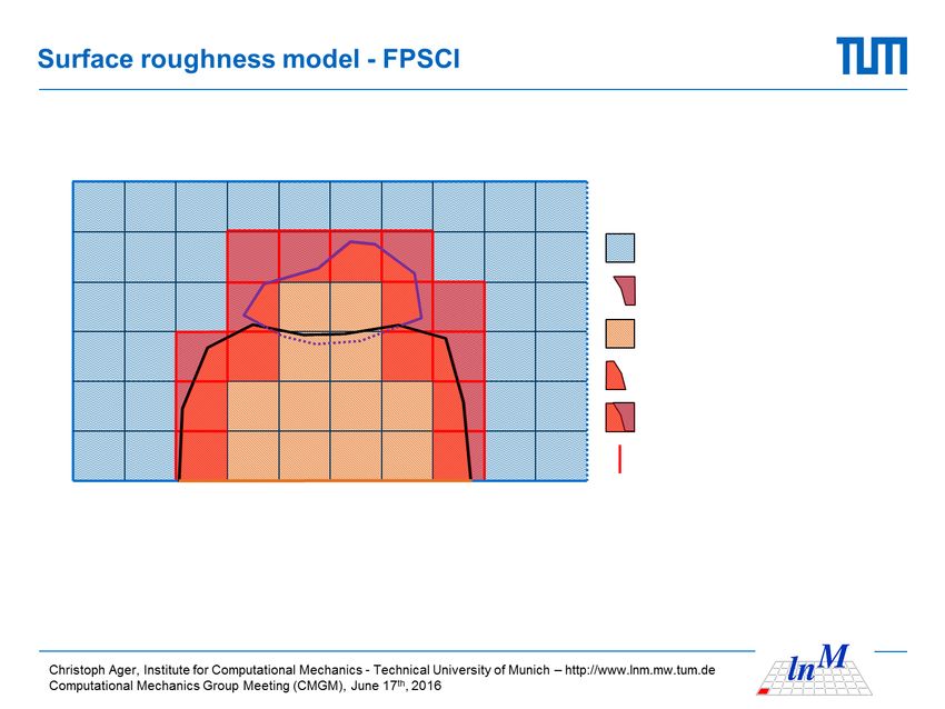
8                                          C. AGER ET AL.

2.3. Conditions on the overall coupling interface Γ in normal direction
For the formulation of the interface constraints, which are splitted in the interface normal direction
and in the tangential plane, the solid outward unit normal n = nS will be considered. The normal
                                                           S
component of the respective Cauchy stress is denoted as: σnn  = σ S : P n and σnn F
                                                                                     = σ F : P n , with
the normal projection operator being specified as P n := n ⊗ n.
  The conditions in the normal direction for purely non-adhesive structural contact configurations
are given by the classical Hertz–Signiorini–Moreau (HSM) conditions:
                           gn := (x̌(x) − x) · n ≥ 0 on       Γ × [t0 , tE ],                     (10)
                                               S
                                              σnn   ≤ 0 on    Γ × [t0 , tE ],                     (11)
                                               S
                                           gn σnn   =0   on   Γ × [t0 , tE ],                     (12)
which ensure the non-penetration, the absence of adhesive contact forces, and the complementarity
between the contact pressure and normal gap gn . To obtain the normal gap gn , the point x̌(x) is
obtained as the projection of x along its normal n onto the opposite solid surface; in the case that
no such projection exists, we assume gn → ∞. All quantities ∗ evaluated at this projection point
will be denoted by a check ∗ˇ.
   In the case contacting bodies are surrounded by fluid, the fluid flow in the contacting zone has
to be considered properly as discussed in the introduction. Applying the classical HSM conditions
(10)-(12) directly would result in the implicit assumption that fluid does not fill the contact zone.
For such a configuration an instantaneous change from zero traction to the traction arising from
the ambient fluid in the contact opening zone on the solid boundary would occur and thus the
formulation of a continuous problem is prohibited. Considering, on the contrary, the presence of
(physically reasonable) fluid in the contact zone (on a smaller length scale and not resolved but just
modeled at the current macroscopic scale) leads to modified HSM conditions, where a lifting of both
bodies occurs for vanishing relative traction of contact (solid) traction and ambient fluid traction.
These conditions result in a continuous problem as the balance of solid and fluid traction is essential
on the common interface of a fluid and a solid. Then, the conditions on the interface Γ formulated
for a specific point x on Γ are:
                                               gn ≥ 0 on      Γ × [t0 , tE ],                     (13)
                                S     F
                               σnn − σnn,E (x)      ≤ 0 on    Γ × [t0 , tE ],                     (14)
                              S     F

                           gn σnn − σnn,E (x)       =0   on   Γ × [t0 , tE ].                     (15)
Condition (13) enforces a positive or vanishing gap gn between two solid bodies. In condition
(14), a negative or vanishing relative traction has to be guaranteed, at least in the case without
adhesive forces that is considered here. Finally, in equation (15), either a vanishing gap in the
contact case of solid-solid interaction or a vanishing relative traction in the case of fluid-structure
interaction is enforced. Additionally, the dynamic equilibrium between two contacting bodies has
to be formulated:
                   S
                  σnn    F
                      − σnn,E     S − σ Fˇ
                              = σˇnn                                 on Γ × [t0 , tE ].           (16)
                                       nn,E

In the contact case, due to the vanishing gap gn , the normal fluid traction equals its projection
  F
σnn,E      Fˇ
       = σnn,E   and therefore the classical dynamic equilibrium between both contacting bodies
                                                                                                S
is recovered. For the fluid-structure interaction case, due to the vanishing relative traction σnn  =
  F
σnn,E , both sides of the equilibrium vanish and as a result equation (16) is automatically fulfilled.
Finally, the mass balance for the motion of solid bodies connected to a fluid domain is given as:

                   rel           ∂u
                  vn := v −            ·n=0                       on ΓF S × [t0 , tE ].          (17)
                                 ∂t
Herein, a vanishing normal relative velocity vnrel is enforced solely on the interface ΓF S , which is
part of the fluid outer boundary ∂ ΩF . Applying an extension to the normal relative velocity vn,Erel
                                                                                                      ,
A CONSISTENT AND COMPREHENSIVE APPROACH FOR FSCI                                  9

this condition is automatically fulfilled on the remaining subset of the interface ΓS,c and hence on
the entire Γ.
Remark 1 (Influence of the fluid extension operator)
It should be highlighted, that conditions (14), (15), and (16) are expressed by an extension of the
fluid stress from the fluid-structure interface ΓF S to the contact interface ΓS,c . The fluid stress
extension has an essential influence only close to the condition changing point/curve (ΓF S ∩ ΓS,c ).
This point is contained in the origin from which the extension is constructed, namely the fluid
domain. Thus, even the application of a simple continuous extension strategy of the fluid stress,
which is by definition more accurate close to the fluid domain, provides a sufficiently accurate
fluid stress representation for a wide range of problem configurations. Still, we would like to
emphasize that the continuous extension operator is considered in this work especially to enable
a clear presentation due to its simplicity. In the case that a more accurate physical fluid solution is
required in the contact zone, alternative extension based strategies can be considered or appropriate
equations to describe the fluid flow in this zone can be solved.

2.4. Conditions on the overall coupling interface Γ in tangential direction
In the tangential direction, frictionless solid-solid contact in combination with the general Navier
boundary condition as a kinematic constraint between solid bodies and the fluid domain is
considered for simplicity of presentation. Then, the following conditions have to be fulfilled on
the interface Γ:

                              σS · n · P t = 0                        on ΓS,c × [t0 , tE ],         (18)
                    σF · n − σS · n · P t = 0                                FS

                                                                      on Γ        × [t0 , tE ],     (19)

                    ∂u      F    F
                 v−    + κσ · n      · Pt = 0                         on ΓF S × [t0 , tE ].         (20)
                    ∂t

Herein, the tangential projection operator is specified by P t := I − n ⊗ n. While condition (18)
represents the vanishing tangential traction component on the contact interface ΓS,c , condition (19)
enforces the dynamic equilibrium between solid and fluid on interface ΓF S . As these two conditions
                                         S,c    FS
can coincide at the common
             F
                              point Γ ∩ Γ           only in the case of a vanishing tangential fluid
traction σ · n · P t = 0 , the general Navier boundary condition (20) with a varying slip length
is applied. This condition includes the no-slip boundary condition for a vanishing slip length κ = 0,
which is the common interface condition, successfully applied for macroscopic problem setups.
Nevertheless, on smaller scales, due to characteristics such as surface roughness or wettability, an
interfacial velocity slip can be observed in a large number of experiments [23]. In this contribution,
the main emphasis of applying the general Navier boundary condition is to guarantee continuity
for transitions between fluid-structure interaction and frictionless contact solid-solid interaction and
to enable a relaxation of the tangential constraint close to the contacting zone. To obtain these
properties, an infinite slip length κ = ∞ is specified close to the common point ΓS,c ∩ ΓF S , whereas
a vanishing slip length still allows the consideration of the no-slip condition for the majority of the
fluid-structure interface ΓF S representing the macroscopic modeling point of view. Further details
on the specification of the slip length κ for the presented formulation are given in Section 3.3.
Remark 2 (Continuity of the formulation considering frictional contact)
It should be pointed out that also for the case when frictional contact is considered, specific treatment
of the tangential constraints will be required to result in a continuous problem. This issue arises due
to the fact, that the fluid wall shear stress on a fluid-structure interface is not automatically equal
to the tangential stress resulting from sliding friction of two contacting structures on a macroscopic
view. In the case of a friction model with vanishing tangential interface traction at the condition
changing point/curve ΓF S ∩ ΓS,c , applying the presented strategy directly results in a continuous
problem also for frictional contact. The presented general Navier conditions yields a zero tangential
fluid traction at the condition changing point ΓF S ∩ ΓS,c . Hence, to ensure continuity, a solid contact
friction model has to provide a vanishing tangential traction at this point as well. For instance, this
10 C. AGER ET AL.
can be achieved using a Coulomb friction law (friction coefficient F) based on the relative normal
S F
stress with the total friction bound F · (σnn − σnn,E ).
3. DISCRETE FORMULATION
In this section, the discrete formulation applied to the numerical solution of the FSCI problem is
presented. The spatial discretization of the continuous problem, presented in the previous section,
is based on the FEM and temporal discretization by the one-step-θ scheme is applied. First, the
semi-discrete weak forms directly derived from the governing equations, including additional fluid
stabilization operators, are given. To account for topological changes in the fluid domain, an
elementary feature occurring for the FSCI problems, the CutFEM is applied to the discretization
of the fluid equations and is thus discussed in the following. Therein, details on the determination
of a consistent discrete set of fluid domain and fluid-structure interface for the contact case are
given. The interface conditions, which are split in normal and tangential direction, are incorporated
by Nitsche-based approaches. For the normal direction, a single continuous interface traction
representation is proposed, automatically incorporating the fluid-structure and contact conditions.
A detailed explanation of the resulting contributions by this normal interface traction is given by
analyzing the different cases. Further, a Nitsche-based formulation to incorporate the tangential
fluid-structure interface condition including potential slip is presented. The specification of the slip
length parameter on the interface to enable a continuous transition from fluid-structure coupling
to frictionless contact is discussed. Finally, all contributions are treated in a single global system
of equations and solved monolithically. Additional details on the solution procedure of the FSCI
problem are given at the end of this section. To shorten the presentation only some aspects that
help understanding the approach are discussed here, while many more details can be found in the
referenced literature for the particular building block methods.
In the following, all quantities, including the primary unknowns, the test functions in the weak
form, the domains and interfaces as well as derived quantities are discretized in space. Still, no
additional index h is added to these discrete quantities for the sake of brevity of presentation. The
expressions (∗, ∗)Ω and h∗, ∗i∂Ω denote the L2 -inner products integrated in the domain Ω and on
the boundary/interface ∂ Ω, respectively.
3.1. Weak forms for the domains ΩS , ΩF
The weak forms for the structural domain W S , the fluid domain W F , and the overall coupled
problem W F S can be derived from equations (1) and (5) - (6), respectively.
∂2u
S S,N
D E
W S [δu, u ] = δu, ρS0 + ∇0 δu, F · S S − δu, ρS0 b̂0 − δu, ĥ0 ,
∂t2 ΩS ΩS
0 ΩS
0 ΓS,N
0
0
(21)
∂v
W F [(δv, δp ) , (v, p )] = δv, ρF + δv, ρF v · ∇v ΩF − (∇·δv, p )ΩF
∂t ΩF
F F,N
D E
+ ( (δv ), 2µ (v ))ΩF − δv, ρF b̂ F
− δv, ĥ F,N
+ (δp, ∇·v )ΩF ,
Ω Γ
(22)
FS S F
W [(δu, δv, δp ) , (u, v, p )] = W [δu, u ] + W [(δv, δp ) , (v, p )]
− hδu, σ n iΓ + δv ∅ , σ n Γ .
| {z }
F S,n F S,t
:=WΓ +WΓ
(23)A CONSISTENT AND COMPREHENSIVE APPROACH FOR FSCI 11
Herein, (δu, δv, δp ) are the corresponding test functions of the primary unknowns (u, v, p ). The
discrete solution space is created by a spatial discretization consisting of elements containing piece-
wise polynomials in an element reference coordinate system which are continuous on the inter-
element boundaries. For the pressure p and for each component of the vector-valued quantities
fluid velocity v and solid displacement u the discrete approximation space is directly constructed
by these functions. All test functions are discretized by the same space as their corresponding
primal unknowns. Modifications of these spaces for the incorporation of strong Dirichlet boundary
conditions on ΓS,D0 and ΓF,D are performed in the usual way. For the structural displacements, an
interface fitted discretization is applied, meaning that the elements fill the entire domain ΩS . Details
on the discretization of the fluid domain, which is non-interface fitted, are given in Section 3.1.2.
Including the unique interface traction σ n , which will be discussed in Sections 3.2 and 3.3, the
respective dynamic equilibrium in normal direction (14), (15), and (16), as well as in tangential
direction (18), and (19) is incorporated directly into the weak form. As the interface conditions
(13)-(20) require a separate treatment of normal and tangential constraints, the normal component
σ nn and the tangential component σ n · P t of the interface traction σ n = σ nn · n + σ n · P t are
treated separately in Sections 3.2 and 3.3.
To extend the interface contribution on ΓF S arising from partial integration of the viscous and
pressure contributions in domain ΩF to the overall interface Γ, an additional definition of the
fluid test functions δv ∅ , δp∅ on the whole interface Γ is consulted. For the additional interface
contributions in (23) vanishing fluid test functions outside of the fluid domain ΩF are considered:
(
(δv, δp ) in ΩF
δv ∅ , δp∅ = (24)
0 otherwise.
3.1.1. Stabilization of the discrete fluid formulation In addition to the naturally arising terms of
the fluid weak form (22), discrete stabilization operators have to be added to control convective
instabilities, to ensure discrete mass conservation, and to guarantee inf-sup stability for equal order
interpolation of velocity and pressure:
WSF [(δv, δp ) , (v, p )] = SvF [δv, (v, p )] + SpF [δp, (v, p )] . (25)
Different realizations of these stabilization operators are possible, including residual-based
stabilization and face-oriented stabilization. In [49] a comparison of various techniques for
stabilization of the incompressible flow problem is given. For the presented numerical examples
in Section 4, face-oriented stabilization operators are chosen (for details see [28]).
3.1.2. The CutFEM utilized for discretization of the fluid domain ΩF As discussed in the
introduction, the CutFEM is applied for the discretization of the fluid domain allowing for a fixed
Eulerian computational mesh. Herein, the boundaries and interfaces of the fluid domain are not
required to match the boundary of the computational discretization. This beneficial feature of the
CutFEM allows the direct handling of large motion or deformation of the solid domain ΩS and
even topological changes of the fluid domain ΩF as it is typically occurring for FSCI problems.
The discretization concept is visualized for an exemplary contacting configuration in Figure 3. The
typical small penetration of contacting solid bodies in the discrete solution is visualized exaggerated
in this figure. This aspect is left aside here and is discussed in detail in Section 3.1.3.
All solid domains ΩS1 and ΩS2 are discretized boundary and interface matching. The fluid
discretization is specified to cover the entire fluid domain ΩF and is not matching to the interface
ΓF S . As shown by the exemplary configuration in Figure 3, the outer boundaries of the fluid domain
often match the discretization boundary, which does not necessarily have to be. Then, the physical
fluid domain ΩF results from “cutting out” the non-fluid domain which is specified by the boundary
of the solid domain ∂ ΩS and potential non matching outer boundaries.
In the following, a brief overview on the most important aspects for application of the CutFEM
to the FSCI problem is given. The treatment of all interface conditions is not included here, but12 C. AGER ET AL.
ΩF = T F ∪ TΓFF S ΓF S
TF
TΓFF S
n T0
TΓ0F S
ΩS = T 0 ∪ TΓ0F S
TΓF S
FΓF S
Figure 3. Basic problem setup for the applied CutFEM, structural domain ΩS = ΩS1 ∪ ΩS2 embedded in
the fluid domain ΩF . A non-interface fitted discretization T = T F ∪ TΓF S ∪ T 0 represents the fluid domain
ΩF by a set of elements in T F and the physical sub-domain TΓFF S of the elements in TΓF S . The non-physical
domain, which equals the structural domain ΩS , consists of a set of elements in T 0 and the non-physical
sub-domain TΓ0F S of the elements in TΓF S . For all inner element faces FΓF S of T F ∪ TΓF S , which are
connected to one element in TΓF S , the “ghost penalty” stabilization is applied.
presented in Sections 3.2 and 3.3. A general overview of this method is given in [50] including
references for further details.
The integration of the L2 -inner products in the fluid weak form (22) has to be performed solely
in the physical fluid domain. This domain is described by the outer fluid boundaries ΓF,D and ΓF,N
as well as the deforming position of the interface ΓF S including its solid outward unit normal
vector n. By separation of the fluid discretization, which is constant in time, in different sets of
elements, the numerical integration of (22) can be realized. The computational fluid mesh consists
of the sets of elements which are not intersected by the interface ΓF S and affiliated to the fluid
domain T F or affiliated to the non-fluid domain T 0 . The set of all remaining elements TΓF S
intersected by the interface ΓF S is split into the physical fluid part TΓFF S and the non-fluid part
TΓ0F S , which can be identified by the unit solid outward solid normal vector n. For the “non-
intersected” elements in TΓFF S standard Gaussian quadrature is applied, whereas no integration has to
be performed on elements in TΓ0F S . For the numerical integration of the physical fluid sub-domain
TΓFF S of the intersected elements, the method described in [51], where the divergence theorem is
utilized repeatedly, is applied. No integration has to be performed on the remaining sub-domain
TΓ0F S .
Due to the arbitrary relative position of the deformed interface ΓF S and the fixed computational
fluid mesh, any geometric intersection configuration has to be treated properly. In fact, intersections
leading to very small contributions of single discrete degrees of freedom to the weak form (22) are
critical. If not handled appropriately, these configurations can lead to an ill-conditioned resulting
system of equations or a loss of discrete stability arising from the weak incorporation of interface
conditions presented in the Sections 3.2 and 3.3. These issues can be tackled by additional weakly
consistent stabilization operators added to the weak form (22). Therein, in principle, any non-
smoothness of the discrete extension of the solution into the non-fluid domain TΓ0F S is penalized.
Single degrees of freedom with vanishing contribution in the weak form (22) are then still defined
by the smooth extension of the solution, even if there is no physical relevance left. This kind of
stabilization is called “ghost penalty” stabilization and was first presented in [29] for the Poisson’s
problem. The method which is applied here for the stabilization of the fluid equations is analyzed in
[28]. The operators (26) added to the fluid weak form therein penalizes jumps of normal derivatives
of the velocity v and the pressure p:
WGF [(δv, δp ) , (v, p )] = Gv (δv, v ) + Gp (δp, p ) . (26)
These operators are integrated on a selected set of inner element faces FΓF S marked in Figure 3 by
red lines.A CONSISTENT AND COMPREHENSIVE APPROACH FOR FSCI 13
I ΩF
I ΓF S ,−
ΓF S ,− IV
III II ΩS 2 IV
ΓS,c ,− II ΓS,c ,− F S
ΓF S ΓF S ,+ ΓS,c ,+ Γ ΩF
∗
ΓS,c ,+
ΓS,c
C>0 C≤0 ΩS 1 C>0 C≤0 C>0 ΩS
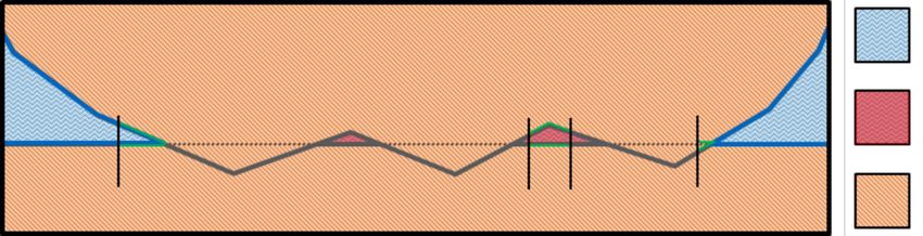
Figure 4. Detailed (exaggerated) view of the discrete contacting zone of two solid bodies ΩS1 and ΩS2 . Due
to the discrete contact formulation, small fluid fractions ΩF∗ can emerge, which are not considered part of the
fluid domain ΩF . The fluid-structure interface ΓF S (blue line) is constructed accordingly to this fluid domain
ΩF . The remaining part of the interface Γ is the contact interface ΓS,c . With the scalar value C introduced in
Section 3.2, the interface is split into four cases (I/ΓF S , −; II/ΓS,c , +; III/ΓF S , +; IV /ΓS,c , −).
Remark 3 (Existence of the discrete fluid test functions in the ghost domain)
It should be highlighted that the discrete test functions (δv, δp ), in contrary to definition (24), do not
vanish in the ghost domain TΓ0F S , and are evaluated on the inter-element faces for the face-oriented
stabilization and “ghost penalty” stabilization (25) and (26) outside of the physical fluid domain ΩF .
3.1.3. Consistent fluid domain ΩF and fluid-structure interface ΓF S representation for the
contacting case The weak form (22) is solely integrated in the physical domain ΩF . This domain
is characterized by the non-moving outer boundaries ΓF,D and ΓF,N as well as the moving fluid-
structure interface ΓF S . The discrete motion of the interface ΓF S is given by the general interface
Γ and hence by the motion of the solid domain ΩS . It is essential to evaluate the overall weak form
on a consistent pair of domain ΩF and interface ΓF S . This aspect is straight-forward as long as
no contact between solid bodies occurs, but should be discussed in detail for the case of contacting
discrete bodies. The contacting scenario illustrated in Figure 4 results in partial overlap of both solid
domain due to the discrete approximation. Therefore, in a first step all parts of the interface Γ which
are overlapping - identified by the solid unit outward solid normal vector n - are removed from
the “intersection” interface. The corresponding fluid domain ΩF ∪ ΩF ∗ potentially includes small
fluid fractions occurring from the discrete contact formulation. To avoid these “islands”, the purely
numerically occurring segments on the current “intersection” interface are removed additionally,
leading to the consulted interface ΓF S . For sufficiently spatially resolved computational meshes, the
identification can be simply performed by a predefined maximal ratio of the element size compared
to the actual size of the bounding box containing a single fluid fraction. Finally, the intersection
of the computational fluid mesh is performed with this interface ΓF S , resulting in a physical fluid
domain ΩF which does not include the domain ΩF ∗ . The discrete contact interface is then defined
by: ΓS,c = Γ \ ΓF S .
3.2. Nitsche-based method on the overall coupling interface Γ in normal direction
The representative interface traction σ nn = σ n · n in normal direction needs to comply with all
interface conditions (13)-(17). Defining the normal interface traction to:
F
+ γEF vn,E
rel
) , (σ Snn + γ S gn ) ,
σ nn = min (σnn,E (27)
with two sufficiently large parameters γEF > 0 and γ S > 0, allows the fulfillment of these conditions
as discussed in the following. The left-hand side of the minimum corresponds to enforcing the FSI
conditions ((14) in the case equal to zero in combination with (17)) and the right-hand side of the
minimum enforces the contact no-penetration condition in normal direction ((13) in the case equal
to zero in combination with (16)). As a result, condition (15) is fulfilled automatically for both
sides of the minimum. If no feasible projection exists, we assume gn → ∞ and as a result the FSI
condition is enforced.14 C. AGER ET AL.
In the case that the contact no-penetration condition is active, the balance of linear momentum
across the closed contact interface, in which condition (16) reduces to σnn S
= σˇnn
S , is accommodated
S
for by using the same representative solid stress σ nn on both sides of the potential contact surfaces.
In the most simple case, one of the two potentially contacting solids, e.g. ΩS1 is designated as a
so-called slave side and the representative solid stress is chosen as the discrete stress representation
of that side σ Snn = σnn S1
. An explicit choice of a slave side, however, results in an inherent bias
between the two solid sides. To obtain an unbiased formulation, an arbitrary convex combination
σ Snn = ωσnn S1
+ (1 − ω )σnn S2
of the stress representations of the two solid sides can be used based on
a weight ω ∈ [0, 1]. If this weight is determined independently of the numbering of the contacting
solids (i.e. invariant with respect to flipping the slave and master side), the resulting algorithm is
unbiased. Two possible choices for unbiased method are either choosing ω = 12 [43, 45] or using
harmonic weights determined based on material parameters and mesh sizes [44, 52].
In the case that the FSI condition is enforced, the normal interface traction is represented uniquely
F
by the normal fluid traction σnn . Thus, the essential dynamic equilibrium (14) in the case equal to
zero and equilibrium (16) due to vanishing contributions on both sides separately are fulfilled . For
this choice, a properly scaled, consistent penalty contribution γ F vnrel is added to guarantee discrete
stability of the formulation and to enforce the constraint (17). In addition to the resulting traction
and penalty contribution, a skew-symmetric adjoint consistency term is added to the weak form
(23):
FS,n rel
WΓ,Adj [(δv, δp ) , (u, v )] = δp∅ n − 2µ (δv ∅ )n, vn,E n Γ
. (28)
This term allows the direct balance of the contribution of the fluid pressure in addition to the viscous
F
contribution, when introducing σnn in (23). Due to the inherent constraint (17), this additional
contribution does not alter the consistency of the formulation. When enforcing the FSI conditions,
also a representation of the interface traction by the corresponding solid stress would be possible,
but is not considered in the following.
A demonstration of the different resulting interface contributions To demonstrate the arising
interface contributions from incorporation of the normal interface traction (27) into the weak form
(23), the boundary integral on the interface Γ is split into the solid-solid contact “+” and the fluid-
structure interaction “−” parts:
( (
h∗, ∗iΓ if C ≤ 0 0 if C ≤ 0
h∗, ∗iΓ,+ = , h∗, ∗iΓ,− = ,
0 otherwise h∗, ∗iΓ otherwise (29)
with C (u, v, p ) = σ Snn + γ S gn − σnn,E
F
+ γEF vn,E
rel
.
Remark 4 (Relation between the interfaces ΓS,c , ΓF S and Γ, +, Γ, −)
For the continuous problem presented in Section 2, integration on the interface subsets Γ, + and
Γ, − coincidences with an integration on the contact interface ΓS,c and the fluid-structure interface
ΓF S , respectively. Due to the discrete error this relation does not hold for the discrete formulation,
where in general a deviation between these interfaces will occur.
In definition (29), the sign of the scalar C indicates, which side of the min[] function in (27)
represents the normal interface traction. In addition to this split of interface Γ in the “+” and
“−” parts, a purely geometric split into interfaces ΓF S and ΓS,c was described in Section 3.1.3.
As the interface ΓF S is part of the outer fluid boundary ∂ ΩF , the fluid state (v, p ) and the
corresponding test functions (δv, δp ) are directly defined on this interface without any extension
required. Combining these two different subdivisions when performing the integration of the normalYou can also read