A global map of root biomass across the world's forests - ESSD

A global map of root biomass across the world’s forests
 Yuanyuan Huang1,2, Phillipe Ciais1, Maurizio Santoro3, David Makowski4,5, Jerome Chave6, Dmitry
 Schepaschenko7,8,9, Rose Z. Abramoff1, Daniel S. Goll1, Hui Yang1, Ye Chen10, Wei Wei11, Shilong
 Piao12,13,14
 5
 1
 Laboratoire des Sciences du Climat et de l'Environnement, LSCE/IPSL, CEA-CNRS-UVSQ, Université Paris-Saclay,
 91191 Gif-sur-Yvette, France.
 2
 Commonwealth Scientific and Industrial Research Organisation, Aspendale, 3195, Victoria, Australia.
 3
 Gamma Remote Sensing, 3073 Gümligen, Switzerland.
10 4
 INRA, AgroParisTech, University Paris‐Saclay, UMR 211, F‐78850 Thiverval‐Grignon, France.
 5
 CIRED, 45bis Avenue de la Belle Gabrielle, 94130 Nogent-sur-Marne, France.
 6
 Laboratoire Evolution et Diversite Biologique UMR 5174, CNRS, Universite Paul Sabatier, 118 route de Narbonne,
 Toulouse, 31062 France.
 7
 International Institute for Applied Systems Analysis (IIASA) Schlossplatz 1, A-2361 Laxenburg, Austria.
 8
15 Center of Forest Ecology and Productivity of the Russian Academy of Sciences, Moscow 117997, Russia
 9
 Siberian Federal University, Krasnoyarsk, 660041, Russia
 10
 Department of Mathematics and Statistics, Northern Arizona University, 86001, Flagstaff, AZ, US.
 11
 State Key Laboratory of Urban and Regional Ecology, Research Center for Eco-environmental Sciences, Chinese
 Academy of Sciences, Beijing, 100085, China.
 12
20 Sino-French Institute for Earth System Science, College of Urban and Environmental Sciences, Peking University, Beijing,
 China
 13
 Key Laboratory of Alpine Ecology and Biodiversity, Institute of Tibetan Plateau Research, Chinese Academy of Sciences,
 Beijing, China
 14
 Center for Excellence in Tibetan Earth Science, Chinese Academy of Sciences,
25 Beijing, China

 Correspondence to: Yuanyuan Huang (yuanyuanhuang2011@gmail.com)

30

 1

Abstract. As a key component of the Earth system, roots play a key role in linking Earth’s lithosphere, hydrosphere,
 biosphere, and atmosphere. Here we combine 10307 field measurements of forest root biomass worldwide with global
 observations of forest structure, climatic conditions, topography, land management and soil characteristics to derive a
 spatially explicit global high-resolution (~ 1km) root biomass dataset, including fine and coarse roots. In total, 142 ± 25
35 (95% CI) Pg of live dry matter biomass is stored below-ground, representing a global average root:shoot biomass ratio of
 0.25 ± 0.10. Our estimations of total root biomass in tropical, temperate and boreal forests are 44-226% smaller than earlier
 studies (Jackson et al., 1997; Robinson, 2007; Saugier et al., 2001), and the total global forest root biomass is 32% smaller
 than a recent estimate (Spawn et al., 2020). The smaller estimation is attributable to the updated forest area, spatially explicit
 above-ground biomass density used to predict the patterns of root biomass, new root measurements and upscaling
40 methodology. We show specifically that the root shoot allometry is one underlying driver that leads to methodological
 overestimation of root biomass in previous estimations. Raw datasets and global maps generated in this study are deposited
 at the open access repository Figshare
 (https://figshare.com/articles/Supporting_data_and_code_for_A_global_map_of_root_biomass_across_the_world_s_forests/
 12199637)

45 1 Introduction

 Roots act as a hub that connects complex feedbacks among biomes, soil, water, air, rocks and nutrients. Roots
 mediate nutrient and water uptake by plants, below-ground organic carbon decomposition, the flow of carbohydrates to
 mycorrhizae, species competition, soil stabilization and plant resistance to windfall(Warren et al., 2015). The global
 distribution of root biomass is related to how much photosynthates plants must invest below-ground to obtain water, nitrogen
50 and phosphorus for sustaining photosynthesis, leaf area and growth. Root biomass and activity also control the land surface
 energy budget through plant transpiration(Wang et al., 2016; Warren et al., 2015). While Earth Observation data combined
 with field data enables the derivation of spatially explicit estimates of above-ground biomass with a spatial resolution of up
 to 30 meters over the whole globe(GlobalForestWatch, 2019; Santoro, 2018b), the global carbon stock and spatial details of
 the distribution of below-ground root biomass (fine + coarse) rely on sparse measurements and coarse extrapolation so far,
55 therefore remaining highly uncertain.
 More than twenty years ago, Jackson et al, 1996, 1997 1,2 provided estimates of the average biomass density (weight
 per unit area) and vertical distribution of roots for 10 terrestrial biomes. Multiplying their average root biomass density with
 the area of each biome results in a global root biomass pool of 292 Pg, with forests accounting for ~68%. Saugier, et al.
 (2001) estimated global root biomass to be 320 Pg by multiplying biome-average root to shoot ratios (R:S) by shoot biomass
60 density and the land area of each biome. Mokany, et al. (2006) argued that the use of mean R:S values at the biome scale is a
 source of error because root biomass measurements are performed at small scales, but root distributions are highly spatially
 heterogeneous and their size distribution spans several orders of magnitude, fine roots being particularly difficult to

 2

sample(Jackson et al., 1996; Taylor et al., 2013). With updated R:S and broader vegetation classes, Mokany, et al. (2006)
 gave a higher global root biomass of 482 Pg. Robinson (2007) further suggested that R:S was underestimated by 60%, which
65 translated into an even higher global root biomass of 540-560 Pg. These studies provided a first order estimation of the root
 biomass for different biomes, but not of its spatial details. Further, it is worth noting that estimations of the global total root
 biomass have increased with time, likely associated with improved methods in excavating roots that reduce under-sampling.
 An alternative approach to estimate root biomass is through allometric scaling, dating back to West, Brown and
 Enquist (1997, 1999)6 7 and Enquist and Niklas (2002). The allometric scaling theory assumes that biological attributes scale
70 with body mass, and in the case of roots, an allometric equation verified by data takes the form of ∝ where R is the root
 mass, S the shoot mass and a scaling exponent. In contrast to the studies listed above assuming the R:S ratio to be uniform,
 this equation implies that the R:S ratio varies with shoot size when β is not equal to one (Cairns et al., 1997; Enquist and
 Niklas, 2002; Jiang and Wang, 2017; McCarthy and Enquist, 2007; Niklas, 2005; Robinson, 2004; Zens and Webb, 2002) .
 Allometric equations also predict that smaller trees generally have a larger R:S with < 1 , which is well supported by
75 measurement of trees of different sizes (Cairns et al., 1997; Jiang and Wang, 2017; Niklas, 2005; Robinson, 2004; Zens and
 Webb, 2002). The allometric equation approach was applied for various forest types, and the scaling exponent was
 observed to differ across sites(Yunjian Luo et al., 2018), species(Cheng and Niklas, 2007), age(Cairns et al., 1997), leaf
 characteristics(Luo et al., 2012), elevation(Moser et al., 2011), management status(Ledo et al., 2018), climatic conditions,
 such as temperature(Reich et al., 2014), soil moisture and climatic water deficit (Ledo et al., 2018), as well as soil nutrient
80 content and texture(Jiang and Wang, 2017). Despite successful application of allometric equations for site- and species-
 specific studies(Yunjian Luo et al., 2018), their use to predict global root biomass patterns appears to be limited and
 challenging.
 2 Methods
 2.1 Overview
85 We use a new approach to upscale root biomass of trees at the global scale (Supplementary Figure 1) based on
 14,30,31
 machine learning algorithms trained by a large dataset of in-situ measurements (n=10307) of root and shoot biomass
 for individual woody plants (see Methods: Field measurement, Supplementary Data), covering 465 species across 10 biomes
 defined by The Nature Conservancy(Olson and Dinerstein, 2002) (Supplementary Figure 2). We compared the allometric
 upscaling and tested three machine learning techniques (the random forest, the artificial neural networks and multiple
90 adaptive regression splines), through a pool of 47 predictor variables that include shoot biomass and other vegetation,
 edaphic, topographic, anthropogenic and climatic variables (Supplementary Table 1). After comparing the results of all three
 machine learning techniques and the allometric upscaling, we chose the random forest model (RF) because it performed best
 on cross validation samples (see section Building predictive models below and Supplementary Table 8), and we only used
 the RF for subsequent mapping and analysis. Using this RF model, we mapped the root biomass of an average tree over an
95 area of ~1km x1 km across the globe using as predictors gridded maps of shoot biomass (weight per area) (Santoro, 2018a),
 tree height(Simard et al., 2011), soil nitrogen(Shangguan et al., 2014), pH(Shangguan et al., 2014), bulk density(Shangguan

 3

et al., 2014), clay content(Shangguan et al., 2014), sand content(Shangguan et al., 2014), base saturation(Shangguan et al.,
 2014), cation exchange capacity(Shangguan et al., 2014), water vapor pressure(Fick and Hijmans, 2017), mean annual
 precipitation(Fick and Hijmans, 2017), mean annual temperature(Fick and Hijmans, 2017), aridity(Trabucco and Zomer,
100 2019) and water table depth(Fan et al., 2013) (Supplementary Figures 10,11,12). Combining our map of root biomass per
 tree with the tree density (number of trees per area)(Crowther et al., 2015) at the global scale, we quantified the global forest
 root biomass.
 2.2 Field measurements
 Our dataset (available at our Figshare repository) was compiled from literature and existing forest biomass structure
105 or allometry databases(Falster et al., 2015) (Ledo et al., 2018; Schepaschenko et al., 2018; Schepaschenko et al., 2017). We
 included studies and databases that reported georeferenced location, root biomass and shoot biomass. Note here we focus on
 studies that measured biomass of individual trees instead of stand level biomass. We included studies that measured biomass
 directly, instead of estimated indirectly via allometric equations. For example, Ref(Poorter et al., 2015) is not included due to
 lack of georeferenced location and Ref(Iversen et al., 2017) in not used as we also need measurements of other plant
110 compartments like shoot biomass. Repeated entries from existing databases were removed. One of the databases(Falster et
 al., 2015) reported data on woody plants which also include shrub species. We kept the shrub data partly because the remote
 sensing products we used to generate our root map do not clearly separate trees from shrubs. Around 82% of the extracted
 entries also recorded plant height and management status. Height was identified as an important predictor in our model
 assessment, and entries were discarded when height was missing (18% of data). As woody plant age was reported in 19% of
115 the entries only, the values of this variable was determined from another source of information, i.e. from a composite global
 map introduced in the next section. Species names were systematically reported, but biotic, climatic, topographic and soil
 information were missing for a substantial proportion of entries and values of these variables were thus extracted from
 independent observation-driven global maps as explained in the next section. Our final dataset includes biomass
 measurements collected in 494 different locations from 10307 individual plants, which cover 465 species across 10 biomes
120 as defined by The Nature Conservancy(Olson and Dinerstein, 2002) (Supplementary Figure 2; Supplementary Data).
 2.3 Preparing predictor variables
 We used 47 predictors that broadly cover 5 categories: vegetative, edaphic, climatic, topographic and anthropogenic
 (Supplementary Table 1). These variables are chosen due to their relevance to root dynamics based on field studies and their
 availability at the global scale. Vegetative variables include shoot biomass, height, age, maximum rooting depth, biome class
125 and species. Edaphic predictors cover soil bulk density, organic carbon, pH, sand content, clay content, total nitrogen, total
 phosphorus, Bray phosphorus, total potassium, exchangeable aluminium, cation exchange capacity, base saturation (BS), soil
 moisture and water table depth (WT). Climatic predictors are mean annual temperature (MAT), mean annual precipitation
 (MAP), the aridity index that represents the ratio between precipitation and the reference evapotranspiration, solar radiation,
 potential evapotranspiration (PET), vapor pressure, cumulative water deficit (CWD=PET - MAP), wind speed, and mean
130 diurnal range of temperature (BIO2, BIO is the abbreviation for WorldClim bioclimatic indicators), isothermality

 4

(BIO2/BIO7) (BIO3), temperature seasonality (BIO4), max temperature of warmest month (BIO5), min temperature of
 coldest month (BIO6), temperature annual range (BIO7), mean temperature of wettest quarter (BIO8), mean temperature of
 driest quarter (BIO9), mean temperature of warmest quarter (BIO10), mean temperature of coldest quarter (BIO11),
 precipitation of wettest month (BIO13), precipitation of driest month (BIO14), precipitation seasonality (BIO15),
135 precipitation of wettest quarter (BIO16), precipitation of driest quarter (BIO17), precipitation of warmest quarter (BIO18),
 precipitation of coldest quarter (BIO19). The topographic variable is elevation. We did not have the slope and aspect as
 topographic factors after a preliminary test which showed minor effect of elevation from our database. We take the
 management status (managed or not) as the anthropogenic predictor. All references are given in Supplementary Table 1. For
 each variable, we collected multiple datasets whenever possible only for uncertainty quantification. For the “central”
140 estimate, we stick to only one set of these predictors considering the quality and coverage of the databases. We favoured the
 database that is known to have higher quality data or covered more predictors that are relevant to our study for consistency.
 As in-situ field measurements of above-ground biomass (AGB) do not offer a full global coverage, gridded shoot
 biomass data were derived from satellite AGB products to predict root biomass at the global scale with a 1km by 1 km
 spatial resolution. The gridded global shoot biomass dataset used in our study has been extensively calibrated with in-situ
145 observations and is currently the most reliable source of information on shoot biomass offering a global coverage(Santoro,
 2018a; Spawn et al., 2020). To derive the shoot or AGB per tree (in unit of weight per tree) to generate spatially explicit
 global root biomass, we combined the GlobBiomass-AGB satellite data product(Santoro, 2018a) ( in unit of weight per unit
 area) with a tree density map (number of trees per unit area)(Crowther et al., 2015). The GlobBiomass dataset was based on
 multiple remote sensing products (radar, optical, LiDAR) and a large pool of in-situ observations of forest variables(Santoro
150 et al., 2015; Santoro, 2018b). The original GlobBiomass-AGB map was generated at 100 m spatial resolution; for this study,
 the map was averaged into a 1 km pixel by considering only those pixels that were labeled as forest (Santoro, 2018b). A
 pixel was labeled as forest when the tree canopy density was larger than 15% according to Hansen et al. (2013)’s dataset
 (hereafter Hansen2013) averaged at 100 m. The 1-km resolution global tree density map was constructed through upscaling
 429,775 ground-based tree density measurements with a predictive regression model for forests in each biome(Crowther et
155 al., 2015). The forest canopy height map took advantage of the Geoscience Laser Altimeter System (GLAS) aboard ICESat
 (Ice, Cloud, and land Elevation Satellite) (Simard et al., 2011). Forest definitions are slightly different among these three
 maps. Forest area of the tree density map was based on a global consensus land cover dataset that merged four land cover
 products (Tuanmu and Jetz, 2014).Crowther et al. (2015) showed the total tree count from tree density map based on the
 Tuanmu and Jetz (2014) land cover is the same as from the Hansen2013 land cover product. The canopy height map used the
160 Globcover land cover map (Hagolle et al., 2005) as reference to define forest land. We approximated the missing values in
 tree density and height (due to mismatches in forest cover) by the mean of a 5x5 window that is centered on the
 corresponding pixel. We quantified the potential impact of mismatches in forest definition by looking into two different
 thresholds: 0% and 30%.
 We merged several regional age maps to generate a global forest age map. The base age map was derived from

 5

165 biomass through age-biomass curve similarly as conducted in tropical regions in ref.(Poulter, 2019).This age map does not
 cover the northern region beyond 35 N. We filled the missing northern region with a North American age map (Pan et al.,
 2011) and a second age map covering China (Zhang et al., 2017). The North American age map represents the year around
 2003 and as a coarse approximation, we added 7 to represent the year 2010. The China age map was derived for the period
 2009-2013. We took it to approximate age values in China around 2010. Remaining missing pixels were further filled with
170 the age map derived from MODIS disturbance observations. For the final step, we filled the remaining pixels with the GFAD
 V1.1 age map(Poulter, 2019). GFAD V1.1 has 15 age classes and 4 plant functional types (PFTs). GFAD V1.1 represents
 the 2000-2010 era. As a coarse approximation, we choose the middle value of each age class and estimated the age as the
 average among different PFTs.
 Detailed information of all ancillary variables is listed in Supplementary Table 1. To stay coherent, we re-gridded
175 each map to a common 1 km x 1 km grid through the nearest neighbourhood method.
 2.4 Building predictive models
 We investigated the performance of the allometric scaling and three non-parametric models: the random forest
 (RF), the artificial neural networks (ANN) and multiple adaptive regression splines (MARS). Allometric upscaling relates
 root biomass to shoot biomass in the form of ∝ . We assume that one universal allometric equation governs (Enquist
180 and Niklas, 2002) biomass partitioning across species without stratifying the data by species. RF is an ensemble machine
 learning method that builds a number of decision trees through training samples(Breiman, 2001). A decision tree is a flow-
 chart-like structure, where each internal (non-leaf) node denotes a binary test on a predictor variable, each branch represents
 the outcome of a test, and each leaf (or terminal) node holds a predicted target variable. With a combination of learning trees
 (models), RF generally increases the overall prediction performance and reduces over-fitting. ANN computes through an
185 interconnected group of nodes, inspired by a simplification of neurons in a brain. MARS is a non-parametric regression
 method that builds multiple linear regression models across a range of predictors.
 Tree shoot biomass from the in-situ observation data spans a wider range than shoot biomass per plant derived from
 global maps (1x10-7 to 8800 vs. 7.9x10-5 to 933 kg/plant). To reduce potential mapping errors, we selected training samples
 with shoot biomass between 5x10-5 and 1000 kg/plant. The medians and means of shoot biomass, root biomass and R:S from
190 the selected training samples are similar to those from the entire database. Also, to reduce the potential impact of outliers, we
 analyzed samples with R:S falling between the 1st and 99th percentiles, which consists of 9589 samples with R:S ranging
 from 0.05 to 2.47 and a mean of 0.47 and a median of 0.36. Sample filtering slightly deteriorated model performance and
 had minor impact on the final global root biomass prediction (145 from whole samples vs.142 Pg from filtered data). We
 chose root biomass as our target variable instead of R:S because big and small trees contribute equally to R:S while big trees
195 are relatively more important in biomass quantification. In our observation database, we have more samples being small
 woody plants (Supplementary Figure 6). We furthermore split the in-situ measured shoot biomass into three groups, namely
 measurements with shoot biomass smaller than 0.1, between 0.1 and 10, and larger than 10 kg/plant, and trained a specific
 model for each class. The rationale behind this splitting is: (1), to remove the bias of small plants from the distribution of in-
 6

situ measured woody shoot biomass (Supplementary Figure 6); (2), to account for the shift of root shoot allometry with tree
200 size(Poorter et al., 2015) (Ledo et al., 2018; Zens and Webb, 2002); (3), to improve the performance of independent
 validation through numerous combinations of splitting trials; (4), and because tests through weighting samples or resampling
 samples (e.g., over-sampling using Synthetic Minority Over-sampling Technique) showed no better performance.
 Model performances were assessed by 4-fold cross-validation using two criteria: the mean absolute error (MAE)
 and the R-squared value (R2). MAE quantifies the overall error while R2 estimates the proportion of variance in root biomass
205 that is captured by the predictive model. We favoured the model with a smallest MAE and a highest R2. For models with
 comparable MAE and R2, we favoured the model with the minimum number of predictors. For non-parametric models,
 starting from a model with all 47 predictors, we sequentially excluded predictors that did not improve model performance
 one after another. The order of removing predictors was random. After a combination of trials, the best model was from RF
 (Supplementary Table 8) and the final set of predictors included shoot biomass, height, soil nitrogen, pH, bulk density, clay
210 content, sand content, base saturation, cation exchange capacity, vapor pressure, mean annual precipitation, mean annual
 temperature, aridity and water table depth. Note the maximum rooting depth had a minor impact on model performance and
 was not selected in the final model. The depth to which roots inhabit varies among species and environment. Our model
 predictions are therefore not specific to a certain soil depth.
 2.5 Generation of the global root biomass map
215 Over an area of 1km x 1km, we assumed a tree with an average shoot biomass follows the RF model trained above.
 Building upon a large set of samples with each field measurement being an outcome of complex local interactions (including
 within-vegetation competition), we implicitly accounted for some sub-pixel variability (e.g., resource competition and
 responses to environmental conditions) on root biomass. Our RF model was built upon individual woody trees. We
 combined the RF model with global maps of selected predictor variables to produce the map of root biomass for an average
220 woody tree which has a unit of weight per tree. This map was multiplied by tree density (number of woody trees per area)
 (Crowther et al., 2015) at 1-km resolution to obtain the final root biomass map with a unit of weight per area (Supplementary
 Figure 1).
 2.6 Uncertainty quantification
 We estimated the overall uncertainty of the root biomass estimates through quantifying errors caused by predicting
225 root biomass at the 1-km resolution (ƞpred) and converting root biomass per tree to root biomass per unit area ( ƞcon). We
 quantified the prediction uncertainty through an ensemble of predictions. We collected 8 additional global predictor datasets
 (3 shoot biomass, 2 soil and 3 climate datasets) (Supplementary Table 2) and carried out 8x4 (4 folds) sets of additional
 predictions replacing the predictors by each of these additional data maps. We calculated the standard deviation among 36
 predictions for each pixel (Supplementary Figure 4a). Converting root biomass from per tree to per area is through the tree
230 density(Crowther et al., 2015). We assumed the coefficient of variation (CV, i.e., the ratio of the standard deviation to the
 mean) in tree density mapping caused the same relative uncertainty in our per unit area root biomass. CV in tree density
 mapping at the biome scale was derived from Ref(Crowther et al., 2015) through dividing uncertainties in quantifying total

 7

tree numbers by the total tree numbers. ƞcon in terms of standard deviation is therefore equal to the product of CV and the
 mean root biomass at each pixel (Supplementary Figure 4b). At last we propagated these two sources of uncertainty
235 assuming these errors were random and independent. Note that we did not account for uncertainties in in-situ root biomass
 measurements used in training the RF model. The overall uncertainty (standard deviation) at the pixel level was calculated
 through,

 ƞ = √ƞ2 + ƞ2 (1)

 At the biome and global scales, we obtained total root biomass for each of the 36 predictions and estimated the standard
240 deviations of the total root biomass. ƞcon was estimated by multiplying CV by biome or global-level root biomass. We
 propagated these two sources of uncertainty through Equation 1. Note that the semivariogram of the random forest prediction
 errors do not show a clear autocorrelation pattern (Supplementary Figure 10).

 2.7 Relative importance of predictor variables
245 The impact of predictors on predicting R:S was estimated through the Spearman's rank-order correlation at both the
 global and biome scales. We log-transformed the R:S and shoot biomass before standardizing these datasets. Partial
 dependence plots(Hastie et al., 2009) show the marginal effect that one predictor has on root biomass from a machine
 learning model, and serves as a supplement to the Spearman correlation.
 3 Results
250 We estimated a global total root biomass of 142±25 (95% CI) Pg (see Methods for uncertainty estimation and
 Supplementary Figures 3, 4) for forests when forest is defined as all areas with tree cover larger than 15% from the Hansen
 et al. (2013) tree cover map. Note here we reported values in unit of Pg of dry biomass instead of Pg C. The corresponding
 global weighted mean R:S is 0.25 ± 0.10. The root biomass spatial distribution generally follows the pattern of shoot
 biomass, but there are significant local and regional deviations as shown by Figure 1. 51% of the global tree root biomass
255 comes from tropical moist forest, 14% from boreal forest, 12% from temperate broadleaf forest and 10% from woody plants
 in tropical and subtropical grasslands, savanna and shrublands (Supplementary Table 3). Given our use of a tree cover
 threshold of 15% at 100m resolution, our estimate ignores the roots of isolated woody plants present in arid or cold regions
 (Staver et al., 2011), as well as heterogeneous (e.g. urban or agriculture) landscapes and is possibly an under-estimate. Total
 root biomass decreases from 151 to 134 Pg when the canopy cover threshold used to define forest land is increased from 0%
260 to 30%. The root biomass density per unit of forest area is highest in tropical moist forest, followed by temperate coniferous
 and Mediterranean forest (Figure 1, Supplementary Table 3). Cross validation showed a good match between predictions
 from our RF model and in-situ observations (Figures 2e, all data; Supplementary Figure 7, for each biome; Supplementary
 Figure 8, for three tree size classes; Supplementary Figure 9, for each continent), with an overall coefficient of determination
 R2 of 0.85, a mean absolute error (MAE) of 2.18 kg and a median R:S similar to validation samples (0.35 from in-situ
265 observation vs. 0.38 from prediction). RF shows better performance than the other two machine learning algorithms and the

 8

allometric fitting, as shown in Supplementary Table 8. By continents, the performance of RF is worst in Africa (R2 = 0.6;
 MAE = 44 kg) partly due to limited observations (Supplementary Figure 9). Root biomass of tropical, temperate and boreal
 forests together is 44-226% lower compared to earlier studies (Table 1, Supplementary Table 5, see Supplementary
 Information Comparison with published results).

270
 Figure 1. Global maps of forest root biomass generated through the random forest model (a), shoot biomass from
 GlobBiomass-AGB(Santoro, 2018b) (b) and R:S (c). Forest is defined as an area with canopy cover > 15% from the Hansen
 et al. (2013) tree cover map.

275 We then analysed the dominant factors explaining spatial variations of root biomass and R:S (see Methods).

 9

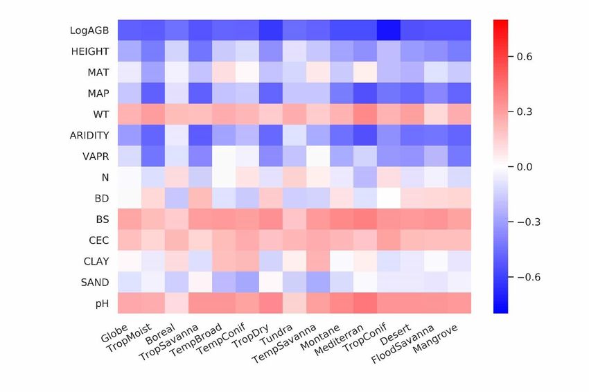
Broadly speaking, locations with small trees, low precipitation, strong aridity, deep water table depth, high acidity, low bulk
 density, low base saturation and low cation exchange capacity are more likely to have higher fractional root biomass (Figure
 3). In line with the allometric theory, shoot biomass emerged as the most important predictor of R:S and root biomass, as
 given by the Spearman correlation analysis shown in Figure 3, and partial importance plots (Supplementary Figures 11, 12,
280 13). Water related variables (precipitation, water table depth, aridity and vapor pressure) also emerged as important
 predictors in explaining R:S patterns (Figure 3)(Ledo et al., 2018), with trees and woody plants in dry regions generally
 having higher R:S (Supplementary Tables 3, 4), and with stronger dependence on precipitation especially when precipitation
 is low and on water table depth when the water table is deep. Temperature is slightly negatively correlated with R:S at the
 global scale, in line with Reich et al. (2014). However, the relationship between temperature and below-ground biomass is
285 not consistent among biomes (Figure 3) and biomass size groups (Supplementary Figures 11, 12, 13).
 The relationship between total soil nitrogen and root biomass is negative when soil nitrogen content is below 0.1-
 0.2 % (Supplementary Figure 11, 12, 13). Root biomass and R:S generally increases with soil alkalinity (Figure 3,
 Supplementary Figures 11, 12, 13). Low pH is toxic to biological activities and roots, especially as fine roots are sensitive to
 soil acidification, as revealed by a recent meta-analysis(Cheng Meng et al., 2019). Our results also indicate overall positive
290 correlations between CEC, BS and R:S, but the processes that may account for these correlations are less clear from
 literature. Age has been shown to be important for R:S(Schepaschenko et al., 2018). How age regulates R:S remains elusive,
 with studies showing both positive(Waring and Powers, 2017) and slightly negative(Mokany et al., 2006) relationship
 between R:S and age. Including forest age (see Methods: Preparing predictor variables) as a predictor only marginally
 improved our model prediction (see Supplementary Information for details). It is likely that shoot biomass partially accounts
295 for age information and the quality of the global forest age data might also affect the power of this variable in improving root
 biomass predictions.

 Table 1. Comparison between studies quantifying root biomass in tropical, temperate and boreal forests.
 This This Jackson(Jackso Saugier(Saugier et Robinson(Robin Spawn (Spawn et al., This study S3
 S1 S2
 study study n et al., 1997) al., 2001) son, 2007) 2020)
 Method Machine Machine Biome average Biome average Biome average Relationships between Allometric
 learning learning root biomass R:S, shoot R:S, shoot root/total biomass and equations
 density biomass density biomass density temperature
 Tropical (Tr, Pg) 92 76 114 147 246
 Temperate(Te, Pg) 26 25 51 59 98
 Boreal (Bo, Pg) 21 20 35 30 50
 Tr + Te + Bo (Pg) 139 121 200 236 394
 Globe (Pg) 142 142 188# 155-210
 RDS1* 0% 44% 70% 183% 32%
 RDS2& 0% 65% 95% 226% 32%

 S1, Tropical moist forest (Biome 1), tropical dry forest (Biome 6), tropical/subtropical coniferous forest (Biome 11) and

 10

300 forest in tropical/subtropical grasslands/savannas and shrublands (Biome 3) are aggregated to represent tropical systems (Tr).
 Temperate broadleaf/mixed forest (Biome 4), temperate coniferous forest (Biome 5) and forest in temperate
 grasslands/savannas and shrublands (Biome 8) are merged together as temperate systems (Te). Boreal forest (Biome 2) and
 woody plants in tundra region (Biome 7) are aggregated as boreal forest (Bo). Biome classification is from The Nature
 Conservancy(Olson and Dinerstein, 2002) and is shown in Supplementary Figure 2.
305 S2, Tropical systems (Tr): Biomes 1,6,11; Temperate systems (Te): Biomes 4,5; Boreal systems (Bo): Biome 2.
 S3, Estimation based on allometric equations and the global above-ground biomass dataset from ref(Santoro, 2018b). See
 Supplementary Table 7 for details.
 #
 This value is converted from 94 Pg C to 188 Pg biomass assuming a 50% carbon content of tree biomass.
 *
 RDS1, the relative difference of Tr + Te + Bo between this study (S1) and previous quantifications. RDS1 = (previous study –
310 this study)/this study x 100%. For example, in the column with the head Jackson, RD S1 = (200-139)/139*100% = 44%.
 &
 RDS2, the same as RDS1, but with the S2 definition of tropical, temperate and boreal systems.

 11

Figure 2. Root biomass and root shoot ratio (R:S). (a) and (b) show as violin plots the distribution of root and shoot biomass
315 (in unit of kg/plant) and R:S ratios in the raw data used for upscaling. (c) and (d) are the distributions of model-predicted
 root biomass from this study, of above-ground biomass used for the prediction, and of modelled R:S ratios at the global and
 biome scales. (e) is a heat plot of observed vs. predicted root biomass in kg of root per individual woody plant (see
 Supplementary Figures 7, 8, 9 for cross-validation at biome, tree size class and continental scales). (f) shows the mean
 (purple) and median (grey) R:S as a function of shoot biomass from observations. A shift of the shoot biomass towards a
320 larger size ((a), (c)) results in a smaller predicted mean R:S at the global scale ((b),(d)) (see Supplementary Table 4 for exact
 values) as the mean R:S is size dependent. R2 is the coefficient of determination, MAE is the mean absolute error and N is the
 number of samples. TropMoist: tropical moist forest; Boreal: boreal forest/taiga; TempBroad: temperate broadleaf and
 mixed forest; TempConif: temperate coniferous forest; Mediterran: Mediterranean forests, woodlands and scrub; TropConif:

 12

tropical and subtropical coniferous forest; and Mangrove forest: mangrove forest. Note that the scales of y-axis are different
325 between (a) and (c), (b) and (d). Model training and prediction were conducted on filtered data with R:S falling between the
 1st and 99th percentiles and shoot biomass matching the range derived from GlobBiomass-AGB(Santoro, 2018b) to reduce
 impacts from outliers.

330

 Figure 3. Spearman rank correlations between predictor variables and log-transferred R:S. Spearman coefficients are shown
 at both the global and biome scales for LogAGB: the logarithm of shoot biomass with base 10; HEIGHT: plant height;
 MAT: mean annual temperature; MAP: mean annual precipitation; WT: water table depth; ARIDITY: the aridity index;
335 VAPR: water vapor pressure; N: soil nitrogen content; BD: soil bulk density; BS: soil base saturation; CEC, soil cation
 exchange capacity; CLAY: soil clay content; SAND: soil sand content; and pH: soil pH. From left to right, biomes are
 ordered by decreasing forest areas (Supplementary Figure 2).
 4 Discussion

 13

Our lower estimation of root biomass compared to earlier studies is attributable to differences in forest area (Supplementary
340 Table 5), above-ground biomass density (Supplementary Table 5), root biomass measurement and upscaling methodology.
 For example, the forest area in temperate zones used in Jackson et al. (1997) was about one third higher than in this study.
 Using the root biomass density (Supplementary Table 5) and estimation method from Jackson et al. (1997), but using the
 updated forest area map from this study, we estimated total root biomass of tropical, temperate and boreal forests to be 147
 Pg (or 184 Pg if sparse forests in tropical/subtropical/temperate grasslands/savannas and shrublands and tundra region are
345 accounted, S1 biome definition in Table 1). This value is smaller than the 200 Pg from Jackson et al. (1997), but still larger
 than the 121 Pg (or 139 Pg ) (Table 1) from our machine learning approach. Our lower values of root biomass compared to
 Saugier et al. (2001), Mokany et al. (2006) and Robinson (2007) are caused mainly by our lower above-ground biomass
 density and R:S (Supplementary Table 5). Shoot or above-ground biomass density (AGB) of tropical zones is 70% lower in
 our study than in Robinson (2007) who used sparse plot data collected more than a decade ago (Supplementary Table 5,
350 case S2), and this lower AGB explains 27-46% of our lower root biomass (Supplementary Tables 5, 6). On the other hand,
 lower biome average R:S explains 41-48% of our underestimation compared to Robinson (2007). To elucidate this
 difference, we calculated weighted biome average R:S ratios through dividing total biome-level shoot biomass by root
 biomass (i.e., weighted mean R:S). These weighted mean R:S, ranging between 0.19 and 0.31 across biomes (Supplementary
 Table 3), are generally smaller than the R:S values reported in previous studies, which were based on average ratios obtained
355 from sparser data (Supplementary Table 5). Note that the arithmetic means R:S (without weighting by biomass) from woody
 plants located in tropical, temperate and boreal zones (Supplementary Table 4) from our database are close to those from
 Robinson (2007) (Supplementary Table 5). And our predicted patterns of relatively large R:S in regions such as dry forests,
 savannas and boreal tundra woodlands (Figure 1c) are in line with data compiled from Mokany et al. (2006) and the 2019
 IPCC refinement (IPCC2019, 2019). Spawn et al. (2020) estimated root biomass from shoot biomass and the correlation
360 between root/total biomass and temperature. Among previous studies, the recent study from Spawn et al. (2020) shows the
 smallest difference from our study. After accounting for sparse forests, the 32% smaller estimation from our study is likely
 linked to differences in the definition of forests and upscaling methodology.
 The common practice of estimating root biomass through an average R:S without considering the spatial variability
 of biomass and this ratio4 is a source of systematic error, leading to overestimating the global root biomass for two reasons.
365 Firstly, upscaling ratios through arithmetic averages (possibly weighted by the number of trees or area, but not accounting
 for the fine-grained distribution of biomass) systematically overestimates the true mean R:S because R:S is a convex
 negative function of S given by : ∝ −1 with taking typical values of about 0.9 (Mokany et al., 2006; West et al.,
 1997, 1999) (see also Supplementary Information: Arithmetic mean R:S section). This explains why high-resolution S data
 used to diagnose weighted mean R:S ratios in our approach give generally smaller values than using arithmetic means across
370 grid cells at the biome level (Weighted R:S Ratio in Supplementary Table 3 vs. Mean (Gridded) in Supplementary Table 4).
 Multiplying this biome-level arithmetic mean R:S by the average biome-level shoot biomass (Supplementary Table 3)
 yielded a global forest root biomass of 155 Pg, larger than 142 Pg. Secondly, available measurements tend to sample more

 14

small woody plants than big trees compared to real world distributions, because small plants are easier to excavate for
 measuring roots (see Figure 2a, 2c) but smaller plants tend to have larger R:S (Figure 2e, see also Refs(Enquist and Niklas,
375 2002) (Zens and Webb, 2002)). This sampling bias shifts the R:S towards larger values. If we use the biome-level mean R:S
 from our in-situ database (Mean (Obs) in Supplementary Table 4), multiplying the shoot biomass (Supplementary Table 3)
 yielded a global value of 233 Pg, larger than using the mean R:S across grid cells through RF (155 Pg). Our RF approach
 uses in-situ data for training but in the upscaling, it accounts for realistic distributions of plant size (Supplementary Figure 5;
 Supplementary Table 4). We further verified that our upscaled R:S ratios are robust to sub-sampling the training data in
380 observed distributions, so that the bias of training data towards small plants does not translate into a bias of upscaled results
 (see Method, Supplementary Figure 8).
 The upscaling approach using allometric equations should also tend to overestimate (see Supplementary
 Information: Allometric upscaling section) the global root biomass due to the curvature of these allometric functions(Enquist
 and Niklas, 2002; Zens and Webb, 2002). The global forest root biomass ranges between 154 – 210 Pg when root biomass
385 was upscaled through different allometric equations collected from literature and fitted to our database (Supplementary
 Table 7), generally larger than from the RF mapping. The global root biomass is likely to be smaller than when applying the
 allometric equation to the spatial average of shoot biomass (Supplementary Figures 14,15,16,17). Thus, future in-situ
 characterization of the distribution of tree sizes across the world’s forests (see Supplementary Information: Allometric
 upscaling section) would greatly improve root biomass quantification. Note that how well our global estimate reflects the
390 real root biomass is conditioned upon the accuracy of in-situ root measurement database used to train our RF model. Under-
 sampling is a common issue in many root studies due the fractal distribution of root systems in soils and the difficulty of
 implementing an efficient sampling strategy(Taylor et al., 2013), especially for large trees. We did not quantify the
 uncertainty of our estimates associated with in-situ root measurements due to lack of reliable information.
 An accurate spatially explicit global map of root biomass helps to improve our understanding of the Earth system
395 dynamics by facilitating fundamental studies on resource allocation, carbon storage, plant water uptake, nutrient acquisition
 and other aspects of biogeochemical cycles. For example, the close correlation (correlation coefficient: 0.8) between root
 biomass and rooting depth(Fan et al., 2017) at the global scale and the importance of roots for plant water uptake and
 transpiration reflect close interactions between vegetation and hydrological cycles. The quest for drivers that affect allocation
 and consumption of photosynthetic production is a major focus of comparative plant ecology and evolution, as well as the
400 basis of plant life history, ecological dynamics and global changes(McCarthy and Enquist, 2007). Turnover time and
 allocation are two key aspects that contribute to large uncertainties in current terrestrial biosphere model predictions(Bloom
 et al., 2016; Friend et al., 2014). Our root biomass map does not provide data on turnover or allocation, but an outcome on
 their aggregated effects. Future studies combining the root biomass map with upscaled root turnover data could shed light on
 the allocation puzzle. The growth of the fast turnover part of roots, mostly fine roots, and leaves are highly linked. If we
405 assume an annual turnover of leaves and fine roots, a preliminary estimation of average forest fine root biomass (from leaf
 biomass) reaches 6.7-7.7 Pg (see Supplementary Information: Preliminary estimation of fine root biomass). Despite being a

 15

small portion of total plant biomass and highly uncertain, fine roots are temporally variable and functionally critical in
 ecosystem dynamics. Future studies on global distribution and temporal dynamics of fine roots are valuable. Considering
 specific biomes, tropical savannas would benefit from better root biomass estimation due to its large land area, and in
410 tropical dry forests, field measurements of root and shoot biomass are needed to refine root biomass quantifications.
 Data availability
 Raw datasets and global maps generated in this study are deposited at the open access repository Figshare
 (https://figshare.com/articles/Supporting_data_and_code_for_A_global_map_of_root_biomass_across_the_world_s_forests/
 12199637) (Huang et al., 2020). The source data and code underlying Figs 1, 2, 3 Supplementary Figs 2-17 are also provided
415 at the Figshare.
 Code availability
 Calculations were conducted through Python 2.7.15 and ferret 6.72. The code is deposited at the open access repository
 Figshare
 (https://figshare.com/articles/Supporting_data_and_code_for_A_global_map_of_root_biomass_across_the_world_s_forests/
420 12199637) (Huang et al., 2020).
 Author contributions
 Y.H. and P.C. designed this study. Y. H., P.C., M.S., J.C and D.S. collected the data. D.M., P.C., M.S., J.C., Y.C. and Y.H.
 discussed analyzing methods. Y.H. conducted the analysis and drafted the manuscript. All authors discussed the results and
 contributed to the manuscript.
425 Competing interests
 The authors declare that they have no conflict of interest.
 Acknowledgements
 Y.H., D.S.G and P.C. received support from the European Research Council Synergy project SyG-2013-610028
 IMBALANCE-P and P.C. and Y.H. from the ANR CLAND Convergence Institute. H.Y., D.S. and M. S. were funded
430 through the ESA Climate Change Initiative BIOMASS project. Collecting Russian data were supported by The Russian
 Science Foundation (project no. 19-77-30015). R.Z.A. received support from the French government grant “Make Our
 Planet Great Again”.
 Reference
 Bloom, A.A., Exbrayat, J.F., van der Velde, I.R., Feng, L., Williams, M. (2016) The decadal state of the
435 terrestrial carbon cycle: Global retrievals of terrestrial carbon allocation, pools, and residence
 times. Proceedings of the National Academy of Sciences of the United States of America 113, 1285-
 1290.
 Breiman, L. (2001) Random forests. Machine Learning 45, 5-32.
 Cairns, M.A., Brown, S., Helmer, E.H., Baumgardner, G.A. (1997) Root biomass allocation in the
440 world's upland forests. Oecologia 111, 1-11.

 16

Cheng, D.L., Niklas, K.J. (2007) Above- and below-ground biomass relationships across 1534
 forested communities. Annals of Botany 99, 95-102.
 Cheng Meng, Dashuan Tian, Hui Zeng, Zhaolei Li, Yi, C., Niu, S. (2019) Global soil acidification
 impacts on belowground processes. Environmental Research Letters, Volume 14, Number 7.
445 Crowther, T.W., Glick, H.B., Covey, K.R., Bettigole, C., Maynard, D.S., Thomas, S.M., Smith, J.R.,
 Hintler, G., Duguid, M.C., Amatulli, G., Tuanmu, M.N., Jetz, W., Salas, C., Stam, C., Piotto, D., Tavani, R.,
 Green, S., Bruce, G., Williams, S.J., Wiser, S.K., Huber, M.O., Hengeveld, G.M., Nabuurs, G.J.,
 Tikhonova, E., Borchardt, P., Li, C.F., Powrie, L.W., Fischer, M., Hemp, A., Homeier, J., Cho, P.,
 Vibrans, A.C., Umunay, P.M., Piao, S.L., Rowe, C.W., Ashton, M.S., Crane, P.R., Bradford, M.A. (2015)
450 Mapping tree density at a global scale. Nature 525, 201-+.
 Enquist, B.J., Niklas, K.J. (2002) Global allocation rules for patterns of biomass partitioning in seed
 plants. Science 295, 1517-1520.
 Falster, D.S., Duursma, R.A., Ishihara, M.I., Barneche, D.R., Fitzjohn, R.G., Varhammar, A., Aiba, M.,
 Ando, M., Anten, N., Aspinwall, M.J., Baltzer, J.L., Baraloto, C., Battaglia, M., Battles, J.J., Bond-
455 Lamberty, B., van Breugel, M., Camac, J., Claveau, Y., Coll, L., Dannoura, M., Delagrange, S., Domec,
 J.C., Fatemi, F., Feng, W., Gargaglione, V., Goto, Y., Hagihara, A., Hall, J.S., Hamilton, S., Harja, D.,
 Hiura, T., Holdaway, R., Hutley, L.S., Ichie, T., Jokela, E.J., Kantola, A., Kelly, J.W.G., Kenzo, T., King, D.,
 Kloeppel, B.D., Kohyama, T., Komiyama, A., Laclau, J.P., Lusk, C.H., Maguire, D.A., le Maire, G.,
 Makela, A., Markesteijn, L., Marshall, J., McCulloh, K., Miyata, I., Mokany, K., Mori, S., Myster, R.W.,
460 Nagano, M., Naidu, S.L., Nouvellon, Y., O'Grady, A.P., O'Hara, K.L., Ohtsuka, T., Osada, N., Osunkoya,
 O.O., Peri, P.L., Petritan, A.M., Poorter, L., Portsmuth, A., Potvin, C., Ransijn, J., Reid, D., Ribeiro, S.C.,
 Roberts, S.D., Rodriguez, R., Saldana-Acosta, A., Santa-Regina, I., Sasa, K., Selaya, N.G., Sillett, S.C.,
 Sterck, F., Takagi, K., Tange, T., Tanouchi, H., Tissue, D., Umehara, T., Utsugi, H., Vadeboncoeur,
 M.A., Valladares, F., Vanninen, P., Wang, J.R., Wenk, E., Williams, R., Ximenes, F.D., Yamaba, A.,
465 Yamada, T., Yamakura, T., Yanai, R.D., York, R.A. (2015) BAAD: a Biomass And Allometry Database
 for woody plants. Ecology 96, 1445-1445.
 Fan, Y., Li, H., Miguez-Macho, G. (2013) Global Patterns of Groundwater Table Depth. Science 339,
 940-943.
 Fan, Y., Miguez-Macho, G., Jobbagy, E.G., Jackson, R.B., Otero-Casal, C. (2017) Hydrologic regulation
470 of plant rooting depth. Proceedings of the National Academy of Sciences of the United States of
 America 114, 10572-10577.
 Fick, S.E., Hijmans, R.J. (2017) WorldClim 2: new 1-km spatial resolution climate surfaces for
 global land areas. International Journal of Climatology 37, 4302-4315.
 Friend, A.D., Lucht, W., Rademacher, T.T., Keribin, R., Betts, R., Cadule, P., Ciais, P., Clark, D.B.,
475 Dankers, R., Falloon, P.D., Ito, A., Kahana, R., Kleidon, A., Lomas, M.R., Nishina, K., Ostberg, S.,
 Pavlick, R., Peylin, P., Schaphoff, S., Vuichard, N., Warszawski, L., Wiltshire, A., Woodward, F.I.
 (2014) Carbon residence time dominates uncertainty in terrestrial vegetation responses to future
 climate and atmospheric CO2. Proceedings of the National Academy of Sciences of the United
 States of America 111, 3280-3285.
480 GlobalForestWatch, (2019) Aboveground live woody biomass density,
 https://data.globalforestwatch.org/datasets/8f93a6f94a414f9588ce4657a39c59ff_1.

 17

Hagolle, O., Lobo, A., Maisongrande, P., Cabot, F., Duchemin, B., De Pereyra, A. (2005) Quality
 assessment and improvement of temporally composited products of remotely sensed imagery by
 combination of VEGETATION 1 and 2 images. Remote Sensing of Environment 94, 172-186.
485 Hansen, M.C., Potapov, P.V., Moore, R., Hancher, M., Turubanova, S.A., Tyukavina, A., Thau, D.,
 Stehman, S.V., Goetz, S.J., Loveland, T.R., Kommareddy, A., Egorov, A., Chini, L., Justice, C.O.,
 Townshend, J.R.G. (2013) High-Resolution Global Maps of 21st-Century Forest Cover Change.
 Science 342, 850-853.
 Hastie, T., Tibshirani, R., Friedman, J. (2009) The Elements of Statistical Learning Data Mining,
490 Inference, and Prediction, Second Edition, Section 10.13.2, Springer.
 IPCC2019, (2019) 2019 Refinement to the 2006 IPCC Guidlines for National Greenhouse Gas
 Inventories. vol. 4 (IPCC National Greenhouse Gas Inventories Programme, 2019).
 Iversen, C.M., McCormack, M.L., Powell, A.S., Blackwood, C.B., Freschet, G.T., Kattge, J., Roumet, C.,
 Stover, D.B., Soudzilovskaia, N.A., Valverde-Barrantes, O.J., van Bodegom, P.M., Violle, C. (2017) A
495 global Fine-Root Ecology Database to address below-ground challenges in plant ecology. New
 Phytologist 215, 15-26.
 Jackson, R.B., Canadell, J., Ehleringer, J.R., Mooney, H.A., Sala, O.E., Schulze, E.D. (1996) A global
 analysis of root distributions for terrestrial biomes. Oecologia 108, 389-411.
 Jackson, R.B., Mooney, H.A., Schulze, E.D. (1997) A global budget for fine root biomass, surface
500 area, and nutrient contents. Proceedings of the National Academy of Sciences of the United States
 of America 94, 7362-7366.
 Jiang, Y.T., Wang, L.M. (2017) Pattern and control of biomass allocation across global forest
 ecosystems. Ecology and Evolution 7, 5493-5501.
 Ledo, A., Paul, K.I., Burslem, D., Ewel, J.J., Barton, C., Battaglia, M., Brooksbank, K., Carter, J., Eid,
505 T.H., England, J.R., Fitzgerald, A., Jonson, J., Mencuccini, M., Montagu, K.D., Montero, G., Mugasha,
 W.A., Pinkard, E., Roxburgh, S., Ryan, C.M., Ruiz-Peinado, R., Sochacki, S., Specht, A., Wildy, D.,
 Wirth, C., Zerihun, A., Chave, J. (2018) Tree size and climatic water deficit control root to shoot
 ratio in individual trees globally. New Phytologist 217, 8-11.
 Luo, Y.J., Wang, X.K., Zhang, X.Q., Booth, T.H., Lu, F. (2012) Root:shoot ratios across China's forests:
510 Forest type and climatic effects. Forest Ecology and Management 269, 19-25.
 McCarthy, M.C., Enquist, B.J. (2007) Consistency between an allometric approach and optimal
 partitioning theory in global patterns of plant biomass allocation. Functional Ecology 21, 713-720.
 Mokany, K., Raison, R.J., Prokushkin, A.S. (2006) Critical analysis of root: shoot ratios in terrestrial
 biomes. Global Change Biology 12, 84-96.
515 Moser, G., Leuschner, C., Hertel, D., Graefe, S., Soethe, N., Iost, S. (2011) Elevation effects on the
 carbon budget of tropical mountain forests (S Ecuador): the role of the belowground
 compartment. Global Change Biology 17, 2211-2226.
 Niklas, K.J. (2005) Modelling below- and above-ground biomass for non-woody and woody plants.
 Annals of Botany 95, 315-321.
520 Olson, D.M., Dinerstein, E. (2002) The Global 200: Priority ecoregions for global conservation.
 (PDF file) Annals of the Missouri Botanical Garden 89:125-126. -The Nature Conservancy, USDA
 Forest Service and U.S. Geological Survey, based on Bailey, Robert G. 1995. Description of the

 18

ecoregions of the United States (2nd ed.). Misc. Pub. No. 1391, Map scale 1:7,500,000. USDA
 Forest Service. 108pp. -The Nature Conservancy (2003), based on Wiken, E.B. (compiler). 1986.
525 Terrestrial ecozones of Canada. Ecological Land Classification Series No. 19. Environment Canada,
 Hull, Que. 26 pp. + map.
 Pan, Y., Chen, J.M., Birdsey, R., McCullough, K., He, L., Deng, F. (2011) Age structure and
 disturbance legacy of North American forests. Biogeosciences 8, 715-732.
 Poorter, H., Jagodzinski, A.M., Ruiz-Peinado, R., Kuyah, S., Luo, Y.J., Oleksyn, J., Usoltsev, V.A.,
530 Buckley, T.N., Reich, P.B., Sack, L. (2015) How does biomass distribution change with size and
 differ among species? An analysis for 1200 plant species from five continents. New Phytologist
 208, 736-749.
 Poulter, B.A., Luiz; Andela, Niels; Bellassen, Valentin; Ciais, Philippe; Kato, Tomomichi; Lin, Xin;
 Nachin, Baatarbileg; Luyssaert, Sebastiaan; Pederson, Niel; Peylin, Philippe; Piao, Shilong; Pugh,
535 Tom; Saatchi, Sassan; Schepaschenko, Dmitry; Schelhaas, Martjan; Shivdenko, Anatoly (2019) The
 global forest age dataset and its uncertainties (GFADv1.1). NASA National Aeronautics and Space
 Administration, PANGAEA, https://doi.org/10.1594/PANGAEA.897392.
 Reich, P.B., Luo, Y.J., Bradford, J.B., Poorter, H., Perry, C.H., Oleksyn, J. (2014) Temperature drives
 global patterns in forest biomass distribution in leaves, stems, and roots. Proceedings of the
540 National Academy of Sciences of the United States of America 111, 13721-13726.
 Robinson, D. (2004) Scaling the depths: below-ground allocation in plants, forests and biomes.
 Functional Ecology 18, 290-295.
 Robinson, D. (2007) Implications of a large global root biomass for carbon sink estimates and for
 soil carbon dynamics. Proceedings of the Royal Society B-Biological Sciences 274, 2753-2759.
545 Santoro, M., Beaudoin, A., Beer, C., Cartus, O., Fransson, J.B.S., Hall, R.J., Pathe, C., Schmullius, C.,
 Schepaschenko, D., Shvidenko, A., Thurner, M., Wegmuller, U. (2015) Forest growing stock volume
 of the northern hemisphere: Spatially explicit estimates for 2010 derived from Envisat ASAR.
 Remote Sensing of Environment 168, 316-334.
 Santoro, M., Cartus, O., Mermoz, S., Bouvet, A., Le Toan, T., Carvalhais, N., Rozendaal, D., Herold, M.,
550 Avitabile, V., Quegan, S., Carreiras, J., Rauste, Y., Balzter, H., Schmullius, C. and Seifert, F. M.. (2018a)
 A detailed portrait of the forest aboveground biomass pool for the year 2010 obtained from
 multiple remote sensing observations. Geophysical Research Abstracts, 20, EGU2018-18932, EGU
 General Assembly 2018.
 Santoro, M.e.a. (2018b) GlobBiomass - global datasets of forest biomass. PANGAEA,
555 https://doi.org/10.1594/PANGAEA.894711.
 Saugier, B., Roy, J., Mooney, H.A. (2001) Estimations of global terrestrial productivity: converging
 toward a single number? In: Terrestrial Global Productivity (eds Roy J, Saugier B, Mooney HA), pp.
 543–556. Academic Press, San Diego.
 Schepaschenko, D., Moltchanova, E., Shvidenko, A., Blyshchyk, V., Dmitriev, E., Martynenko, O., See,
560 L., Kraxner, F. (2018) Improved Estimates of Biomass Expansion Factors for Russian Forests.
 Forests 9.

 19

Schepaschenko, D., Shvidenko, A., Usoltsev, V., Lakyda, P., Luo, Y.J., Vasylyshyn, R., Lakyda, I.,
 Myklush, Y., See, L., McCallum, I., Fritz, S., Kraxner, F., Obersteiner, M. (2017) A dataset of forest
 biomass structure for Eurasia. Scientific Data 4.
565 Shangguan, W., Dai, Y.J., Duan, Q.Y., Liu, B.Y., Yuan, H. (2014) A global soil data set for earth system
 modeling. Journal of Advances in Modeling Earth Systems 6, 249-263.
 Simard, M., Pinto, N., Fisher, J.B., Baccini, A. (2011) Mapping forest canopy height globally with
 spaceborne lidar. Journal of Geophysical Research-Biogeosciences 116.
 Spawn, S.A., Sullivan, C.C., Lark, T.J., Gibbs, H.K. (2020) Harmonized global maps of above and
570 belowground biomass carbon density in the year 2010. Scientific Data 7.
 Staver, A.C., Archibald, S., Levin, S.A. (2011) The Global Extent and Determinants of Savanna and
 Forest as Alternative Biome States. Science 334, 230-232.
 Taylor, B.N., Beidler, K.V., Cooper, E.R., Strand, A.E., Pritchard, S.G. (2013) Sampling volume in root
 studies: the pitfalls of under-sampling exposed using accumulation curves. Ecology Letters 16,
575 862-869.
 Trabucco, A., Zomer, R. (2019) Global Aridity Index and Potential Evapotranspiration (ET0)
 Climate Database v2. figshare. Dataset.
 Tuanmu, M.N., Jetz, W. (2014) A global 1-km consensus land-cover product for biodiversity and
 ecosystem modelling. Global Ecology and Biogeography 23, 1031-1045.
580 Wang, Y.Y., Xie, Z.H., Jia, B.H. (2016) Incorporation of a dynamic root distribution into CLM4.5:
 Evaluation of carbon and water fluxes over the Amazon. Advances in Atmospheric Sciences 33,
 1047-1060.
 Waring, B.G., Powers, J.S. (2017) Overlooking what is underground: Root:shoot ratios and coarse
 root allometric equations for tropical forests. Forest Ecology and Management 385, 10-15.
585 Warren, J.M., Hanson, P.J., Iversen, C.M., Kumar, J., Walker, A.P., Wullschleger, S.D. (2015) Root
 structural and functional dynamics in terrestrial biosphere models - evaluation and
 recommendations. New Phytologist 205, 59-78.
 West, G.B., Brown, J.H., Enquist, B.J. (1997) A general model for the origin of allometric scaling
 laws in biology. Science 276, 122-126.
590 West, G.B., Brown, J.H., Enquist, B.J. (1999) A general model for the structure and allometry of
 plant vascular systems. Nature 400, 664-667.
 Yunjian Luo, Xiaoke Wang, Zhiyun Ouyang, Fei Lu, Liguo Feng, Tao, J. (2018) ChinAllomeTree 1.0.
 Zens, M.S., Webb, C.O. (2002) Sizing up the shape of life. Science 295, 1475-1476.
 Zhang, Y., Yao, Y.T., Wang, X.H., Liu, Y.W., Piao, S.L. (2017) Mapping spatial distribution of forest
595 age in China. Earth and Space Science 4, 108-116.

 20