A new island scale tropical cyclone outlook for southwest Pacific nations and territories - Nature
←
→
Page content transcription
If your browser does not render page correctly, please read the page content below
www.nature.com/scientificreports
OPEN A new island‑scale tropical cyclone
outlook for southwest Pacific
nations and territories
Andrew D. Magee1*, Andrew M. Lorrey2, Anthony S. Kiem1 & Kim Colyvas3
The southwest Pacific (SWP) region is vulnerable to tropical cyclone (TC) related impacts which
adversely affect people, infrastructure and economies across several nations and territories. Skilful
TC outlooks are needed for this region, but the erratic nature of SWP TCs and the complex ocean–
atmosphere interactions that influence TC behaviour on seasonal timescales presents significant
challenges. Here, we present a new TC outlook tool for the SWP using multivariate Poisson regression
with indices of multiple climate modes. This approach provides skilful, island-scale TC count outlooks
from July (four months ahead of the official TC season start in November). Monthly island-scale TC
frequency outlooks are generated between July and December, enabling continuous refinement of
predicted TC counts before and during a TC season. Use of this approach in conjunction with other
seasonal climate guidance (including dynamical models) has implications for preparations ahead of
severe weather events, resilience and risk reduction.
The southwest Pacific (SWP; 0°–35°S, 135°E–120°W) is a vast region, home to a number of diverse island nations
and territories that are vulnerable to the impact of natural disasters. Tropical cyclones (TCs) account for 76%
of disasters within the SWP r egion1, which bring extreme winds, intense storm surge, coastal inundation, and
prolonged and intense rainfall that induces landslides and flooding2–4. The relative isolation of SWP islands, their
high shoreline to land area r atio5 and the low relief of coral atolls and fringes of volcanically composed i slands6
that are occupied by people further amplifies physical impacts from TCs. In addition, slow economic g rowth6,
fragile infrastructure7, and a dependence on subsistence f arming8–10 as a single primary industry has resulted
in limited adaptive capacity and slower recovery times from TC impacts11. On ex-tropical transition, TCs have
also had significant impacts on Australia12 and New Zealand13. Several severe TCs have wreaked havoc in the
SWP in recent decades, devastating communities, lives and economies in the r egion14–16.
Provision of accurate and timely seasonal TC outlooks are essential for informed decision making by Pacific
Island National Meteorological Services (PINMS), disaster managers and community stakeholders. For the SWP
region, three seasonal TC outlooks are currently operational: (1) one produced by the National Institute for Water
and Atmospheric Research (NIWA)17 that is distributed through the Island Climate Update18, (2) one from the
Australian Bureau of Meteorology (BOM)19 and one produced by (3) the Fiji Meteorological Service (FMS)20.
The BOM provides outlooks for two regions in the SWP, the western region (142.5°E–165°E) and the eastern
region (165°E–120°W). Both NIWA and the FMS provide seasonal TC outlooks covering exclusive economic
zone (EEZ) scales for SWP islands. Their products are based on selecting historical (analogue) TC seasons with
similar oceanic and/or atmospheric conditions leading up to and what is expected for the season ahead. TCs
within these analogue approaches are composited to infer possible conditions for the upcoming TC season and
include overall TC counts, interactions of TCs with individual countries and a projection of severe TCs for the
season. Each of these organisations employs a different method to derive their TC outlooks, and each considers
different indices to capture ocean–atmosphere variability associated with El Niño-Southern Oscillation (ENSO).
Although ENSO is the leading mode of climate variability across the tropical Pacific21, it has exceptionally
diverse characteristics and flavours (e.g. ENSO Modoki22,23) and can manifest in many different ways, both spa-
tially and temporally24. Coupled ocean-atmospheric processes associated with ENSO influence changes in the
location of favourable thermodynamic conditions that support tropical c yclogenesis25,26 , in particular guiding
1
Centre for Water, Climate and Land (CWCL), University of Newcastle, Newcastle, Australia. 2Climate, Atmosphere
and Hazards Centre, National Institute for Water and Atmospheric Research (NIWA) LTD, Auckland, New
Zealand. 3School of Mathematical and Physical Sciences, University of Newcastle, Newcastle, Australia. *email:
andrew.magee@newcastle.edu.au
Scientific Reports | (2020) 10:11286 | https://doi.org/10.1038/s41598-020-67646-7 1
Vol.:(0123456789)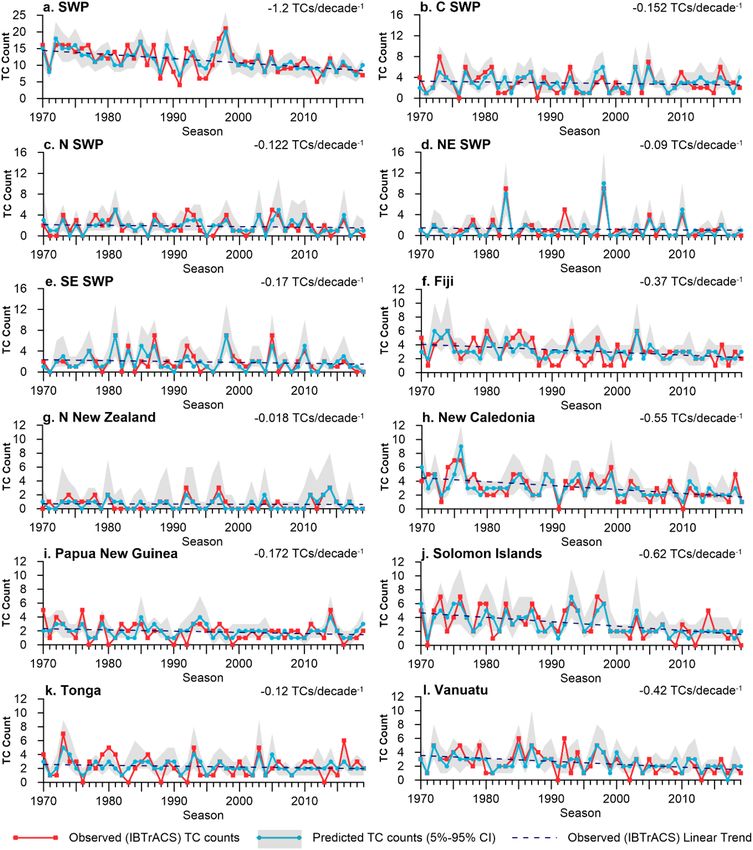
www.nature.com/scientificreports/
the South Pacific Convergence Zone27,28 TC incubation area systematically towards the northeast (southwest)
during El Niño (La Niña) e vents23,29,30. Temporally, El Niño (La Niña) events also result in more (less) TCs during
the SWP TC season, and El Niño conditions are also found to delay the onset of the following SWP TC season30.
The diversity of ENSO means that the most suitable ENSO index/indices to underpin SWP TC outlooks may
vary according to location and time of year. While numerous ENSO indices exist31–36, there is no consensus on
which one best captures the ENSO p henomenon37.
Of importance, ENSO is not the only climate mode to influence SWP TC behaviour. Indian Ocean SST
variability38 is associated with driving spatio-temporal changes in the characteristics of Australian39,40 and SWP
TCs41, in conjunction with, and independent of, E NSO42. The co-occurrence of El Niño (La Niña) and warm
(cool) SSTs in both the IOD E and IOD W regions38 of the tropical Indian Oceans results in significantly greater
modulations of TC activity towards the northeast (southwest), compared to modulations observed through
analysis of ENSO alone. The interplay between ENSO and Indian Ocean SST variability has been shown to result
in substantially different risk profiles for SWP nations and t erritories42. Also, a synergy between the Southern
Annular Mode (SAM) and ENSO shows an increased number of TCs undergo ex-tropical transition reaching
further south during positive SAM and La Niña conditions, which is important for New Zealand43. Considering
multivariate prediction schemes have the potential to produce more robust f orecasts44,45, a combination of cli-
mate influences (ENSO, Indian Ocean SST variability and SAM) is highly relevant, but yet to be formally tested.
We demonstrate an approach for deriving skilful, statistically-driven island-scale TC outlooks for the SWP
that incorporates ENSO with other modes of variability. Several climate indices representing inter-annual Indo-
Pacific climate variability were harnessed with automated variable selection techniques to determine the most
appropriate combination of model predictors for island-scale models. We also recognise the potential of addi-
tional lead time for island-scale TC outlooks is significant for PINMS, as it can enable improved decision-making
for preparedness measures that can reduce TC-related risks (e.g. loss of life and infrastructure). As such, we also
evaluated how changing lead times influences model skill using this approach, and compared model skill for
outlooks derived in October (similar to the release timing for current operational products discussed above),
with outlooks generated up to four months ahead of the TC season. In-season TC outlook updates (Novem-
ber–January) were also tested to determine whether refinements of TC counts for the remainder of the TC
season improved efficacy.
Results
Deriving regional, sub‑regional and island‑scale TC count outlooks. In total, 12 sub-regional and
island-scale outlooks are derived for the SWP region, including a regional SWP model (see Fig. 1). The western
portion of the SWP is particularly active (Fig. 1a), which supported our investigation into individual island-scale
models for Fiji, Solomon Islands, New Caledonia, Vanuatu, Papua New Guinea and Tonga (November–April
seasonal TC climatologies with > 1.5 TCs; see Data and Model Development section). As the eastern SWP is
comparatively less active than the western SWP, EEZs in that region have been grouped together to increase the
number of TC counts for sub-regional models. Our groupings have resulted in four sub-regional outlook areas:
N SWP, C SWP, NE SWP and SE SWP (see Fig. 1b).
In this study, we evaluated the performance of 10 predictor models to produce TC outlooks, each of which
pairs a unique ENSO index with the Marshall SAM index47, Indian Ocean Dipole East Box (IOD E), Indian Ocean
Dipole West Box (IOD W) and the Dipole Mode Index (DMI)38 (see Data and Model Development and Figure S1
(supplementary) for a time series of each index used in this analysis). For predictor models 1–10 (see Table 1),
an automated model selection algorithm is used to select the optimum combination of predictors (indices and
lagged periods), using a generalised linear model with a Poisson distribution and log link function to model the
predicted mean TCs per season for each location. Upon initiating each predictor model using the methodology
as outlined in the Data and Model Development section, the model that generates the highest skill score (SS) is
selected for further analysis.
For TC outlooks initiated in October, the best performing models demonstrate statistically significant skill in
estimating TC counts (Fig. 2), with the robustness of each model tested and cross-validated through a four-stage
model calibration process (Table 2). For outlooks initiated in October, all ENSO indices (except for the Coupled
ENSO Index (CEI)) were selected using the automated model selection algorithm. Of all models, the Trans Nino
Index (TNI) was identified in four target areas as the most effective ENSO indicator for October initiated out-
looks (SWP, N SWP, New Caledonia and the Solomon Islands), when combined with SAM, IOD E, IOD W and
DMI. The methodology used to derive the TNI (the difference in normalised SST anomalies between NINO1 + 2
and NINO4)48, quantifies the gradient in SST anomalies between the central and eastern equatorial Pacific. Its
performance in this analysis may be driven by its ability to quantify some diversity associated with ENSO events,
particularly central Pacific (Modoki) ENSO events. For the Solomon Islands (3.12 TCs per season), model cor-
relations of up to r = 0.79 (p = < 0.0001, n = 50) are observed, with exact strike rates (SR-E; where the outlook,
rounded to the nearest count, exactly matches the observation) of 40% (20 in 50 TC seasons) and SR ± 1 (where
the outlook matches the observation ± 1 TC) of 76% (38 of 50 TC seasons). Sub-regional models also perform
well and demonstrate skill in predicting TCs in regions with fewer TC events. For example, the NE SWP region
(1.22 TCs per season on average) has model correlations of up to r = 0.91 (p = < 0.0001, n = 50), SR-E of 52% (26
in 50 TC seasons) and SR ± 1 of 98% (49 in 50 TC seasons). This provides meteorological services in the Cook
Islands, French Polynesia and Kiribati with enhanced, location-specific outlooks.
Across all regional, sub-regional and island-scale models, TC count outlooks using Poisson regression are able
to replicate the temporal variability and trends of observed TC counts (Fig. 3). The results capture particularly
active (1998) and inactive (1991) TC seasons, as well as the decrease of TC numbers across all model target areas
Scientific Reports | (2020) 10:11286 | https://doi.org/10.1038/s41598-020-67646-7 2
Vol:.(1234567890)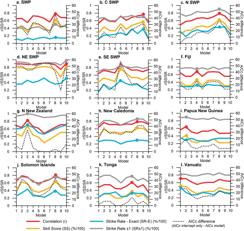
www.nature.com/scientificreports/
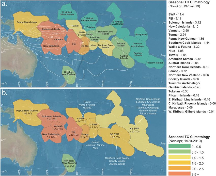
Figure 1. Panel a: Exclusive Economic Zones (EEZ) considered in this study with the shading seasonal TC
climatology (Nov–Apr) between 1970 and 2019. Contours represent seasonal (Nov–Apr) TC track density
between 1970 and 2019 (0.5 TCs/season intervals). Panel b: Location of 12 regional, sub-regional and island
scale models (including entire SWP region: 0°–35°S, 135°E–120W). Where individual EEZ climatology was < 1.5
TCs per season, surrounding EEZs were merged to form the following sub-regions: Northern SWP (N SWP;
Tuvalu, Wallis & Futuna and Tokelau), Central SWP (C SWP; Samoa, American Samoa and Niue), Northeast
SWP (NE SWP; Northern Cook Islands, E.Kiribati: Line Islands, Marquesas, Tuamotu Archipelago, Gambier
Islands and Pitcairn Islands), and Southeast SWP (SE SWP; Southern Cook Islands, Society Islands and Austral
Islands). Island-scale models were derived for the following: Papua New Guinea, Solomon Islands, Vanuatu,
New Caledonia, Fiji, Tonga and Northern New Zealand. Models for W.Kiribati: Gilbert Islands and C.Kiribati:
Phoenix Islands have not been derived or included as part of a larger sub-region as these locations have a low
seasonal TC climatology (≤ 0.06 TCs) and are at minimal risk of TC activity. Figure created using a basemap
from Natural Earth (www.naturalearthdata.com) and EEZ boundaries f rom46.
within the larger SWP that experienced a decrease of up to 1.2 TCs/decade−1 between 1970 and 2019. Although
models are trained on the entire observational time series, fourfold validation was chosen intentionally to evaluate
how the prediction performed when trained on one half and validated on the remaining half of the 50-year time
series. For New Caledonia, calibrating the model on the first (second) half and validating on the second (first)
produces statistically significant correlations of r = 0.76 (r = 0.83) and r = 0.71 (r = 0.59) respectively (p = < 0.0001,
n = 50 for all correlation values). The nature of this cross-validation method means it is particularly sensitive to
linear trends, resulting in some non-significant validation correlations. This would not necessarily be the case
for a leave-one-out cross validation (LOOCV), where the model would typically be calibrated on a much longer
time period (typically n-1). Analysis of model undercount and overcount (Fig. 4), does not suggest a bias towards
consistently underestimating or overestimating TC counts in a given region, nor does it reveal any bias towards
a particular phase of ENSO.
Testing model performance for monthly pre‑season and in‑seasonTC outlook updates. Increas-
ing TC outlook lead time by up to an additional three months (initialisation between July–September instead
of October) can produce skilful and useful estimates of forthcoming TC activity (Fig. 5). For five out of twelve
outlooks, pre-season outlook models achieved better SR-E performance when they were initiated in July versus
Scientific Reports | (2020) 10:11286 | https://doi.org/10.1038/s41598-020-67646-7 3
Vol.:(0123456789)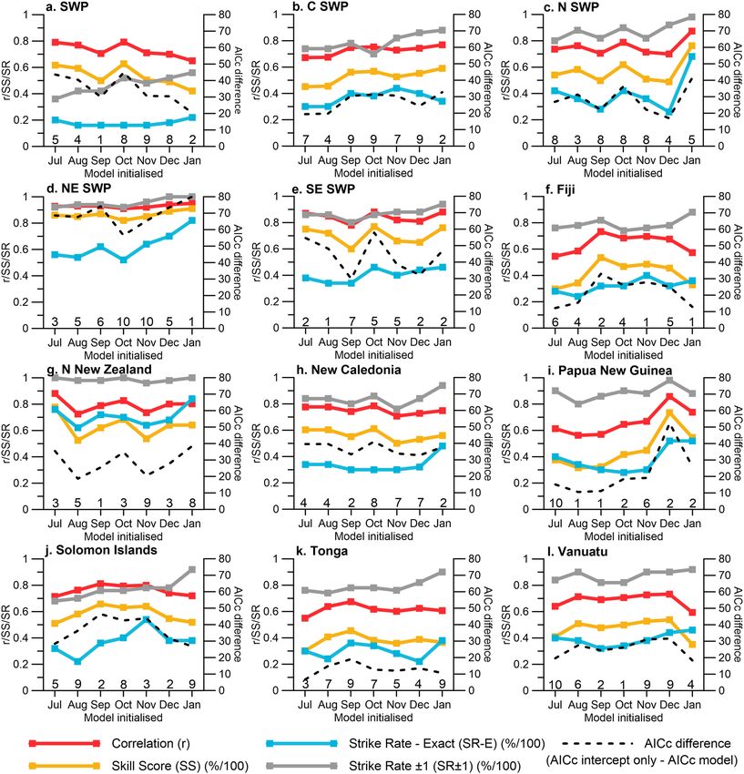
www.nature.com/scientificreports/

                                       Model    ENSO index                     Other indices
                                       1        NINO1 + 2
                                       2        NINO3
                                       3        NINO3.4
                                       4        NINO4
                                                                                 Southern Annular Mode (SAM)
                                       5        Southern Oscillation Index (SOI) IOD E
                                       6        Coupled ENSO Index (CEI)         IOD W
                                                                                 Dipole Mode Index (DMI)
                                       7        Oceanic Nino Index (ONI)
                                       8        Trans Nino Index (TNI)
                                       9        ENSO Modoki Index (EMI)
                                       10       ENSO Longitude Index (ELI)

                                      Table 1.  Ten covariate models used in analysis. Monthly averaged lags (lags 1–6) are generated for each
                                      outlook model initiation period. Individual ENSO indices are combined with other indices including SAM,
                                      IOD E, IOD W and DMI. See the Data and Model Development Section and Fig. 6 for more details on the
                                      indices considered in this analysis.

                                      Figure 2.  Evaluation of predictor model skill for outlooks initialised in October for the November–April TC
                                      season (see Table 1 for predictor model summary). Dots indicate models with superior model performance
                                      based on highest SS.

          Scientific Reports |   (2020) 10:11286 |                 https://doi.org/10.1038/s41598-020-67646-7                                        4

Vol:.(1234567890)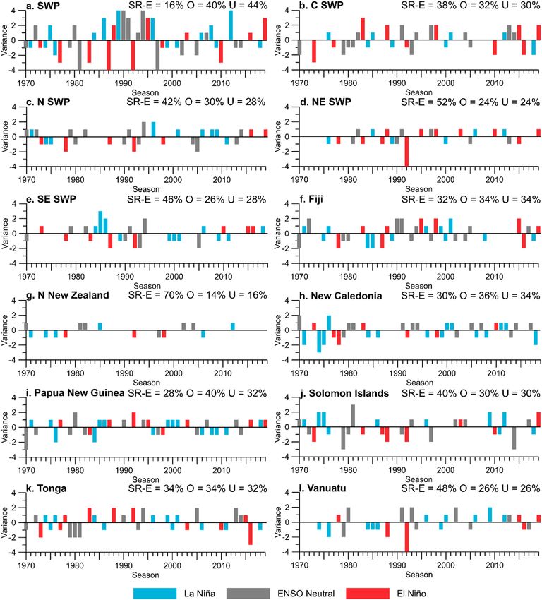
www.nature.com/scientificreports/
Sub-regional models Island-scale models
Papua New Solomon
SWP C SWP N SWP NE SWP SE SWP Fiji N New Zealand New Caledonia Guinea Islands Tonga Vanuatu
Model number 8 9 8 10 5 4 3 8 2 8 7 1
Correlation (r) 0.79* 0.75* 0.79* 0.91* 0.88* 0.68* 0.83* 0.78* 0.65* 0.79* 0.62* 0.70*
Coefficient of
determination 0.63 0.57 0.62 0.82 0.77 0.47 0.69 0.62 0.42 0.63 0.8 0.50
(r2)
RMSE 2.30 1.28 0.97 0.73 0.89 1.17 0.50 1.09 0.99 1.24 1.27 1.10
Skill score (SS)
62.7 56.7 61.9 82.1 77.25 46.7 68.4 61.08 41.67 63.05 38.03 49.63
(%)
Strike rate-exact
16 38 42 52 46 32 70 30 28 40 34 48
(SR-E) (%)
Strike rate-± 1
52 70 90 98 86 74 100 86 90 76 78 82
(SR ± 1) (%)
229.37 171.24 143.26 130.86 140.35 162.07 78.48 155.38 145.27 167.77 169.90 156.40
AICc
274.76 202.54 179.46 187.42 198.25 188.07 113.19 196.41 163.80 210.32 182.58 182.62
AICc difference
(intercept only- 45.39 31.30 36.20 56.56 57.90 26.00 34.71 41.03 18.53 42.55 12.68 26.22
model)
Calibrate 1 0.84* 0.89* 0.85* 0.94* 0.92* 0.74* 1.00* 0.76* 0.67* 0.85* 0.65* 0.67*
1970–1994 2.03 0.97 0.82 0.70 0.81 1.17 0.00 1.17 1.14 11.05 1.41 1.24
Validate 1 0.56* 0.20 0.58* 0.64* 0.41^ 0.31 0.08 0.71* 0.38^ 0.29 0.35 0.64*
1995–2019 2.96 1.75 1.29 1.58 1.78 1.25 0.97 1.08 0.96 1.68 1.28 0.93
Calibrate 2 0.96* 0.91* 0.91* 0.99* 0.97* 0.70* 1.00* 0.83* 0.74* 0.89* 0.76* 0.84*
1995–2019 0.99 0.74 0.65 0.29 0.48 0.94 0.00 0.86 0.70 0.80 0.89 0.67
Validate 2 0.45^ 0.53* 0.33 0.34 0.14 0.49* 0.08 0.59* 0.18 0.31 0.48^ 0.25
1970–1994 3.37 1.83 1.50 1.96 2.05 1.51 0.87 1.45 1.50 1.88 1.64 1.62
Calibrate 3 0.86* 0.86* 0.87* 0.95* 0.99* 0.79* 1.00* 0.82* 0.84* 0.83* 0.82* 0.77*
1982–2006 1.71 1.01 0.77 0.38 0.23 0.90 0.00 1.14 0.87 1.28 1.01 0.92
Validate 3
0.45^ 0.29 0.47^ 0.85* 0.39^ 0.40^ 0.11 0.15 0.39^ 0.38^ 0.37 0.48^
1970–1981 and
3.80 1.87 1.46 1.40 2.14 1.63 0.88 1.55 0.90 1.70 1.34 1.49
2007–2019
Calibrate 4
0.85* 0.90* 0.88* 0.90* 0.95* 0.84* 1.00* 0.89* 0.53* 0.90* 0.81* 0.71*
1970–1981 and
2.26 0.86 0.80 1.14 0.72 0.95 0.00 0.70 0.83 0.79 0.84 1.19
2007–2019
Validate 4 0.25 0.24 0.48^ 0.63* 0.32 0.49* 0.27 0.42^ 0.43^ 0.53* 0.18 0.42^
1982–2006 3.28 1.90 1.36 0.91 1.53 1.28 0.90 1.82 1.43 1.93 1.71 1.30
Table 2. Summary statistics for outlook models initiated in October for the SWP TC season (November–
April). Pearsons correlation coefficient (r), coefficient of determination ( r2), root mean square error (RMSE),
skill score (%), strike rate-exact (SR-E) (%), strike rate ± 1 (SR ± 1) (%) and finite corrected AIC ( AICC)
summarise the performance of the derived models. For AICc, model performance (top value) is compared
with the intercept only model (bottom value). Four stage twofold model validation statistics are also
summarised. Correlation between IBTrACS (observed) and predicted TCs (top value) and RMSE (bottom
value) summarise model performance. ^Correlation significant at 95% level. *Correlation significant at 99%
level.
October, e.g. SWP (24% versus 16%), NE SWP (56% versus 52%), Northern New Zealand (76% versus 70%) and
Papua New Guinea (40% versus 28%). For Northern New Zealand, TC outlooks initiated in July also see higher
correlation and skill score (SS) values (r = 0.88 and 78%), compared to outlooks initiated in October (r = 0.83 and
68%) (p = < 0.0001, n = 50 for both correlation values). While other regions do not see improvements in model
performance with increased lead time when seasonal outlooks initiated in July are compared with those initiated
in October, the models initiated in July still perform well.
Model performance of in-season TC outlooks (November–January) is also tested. In-season TC guidance
updates offers an opportunity to refine outlooks for the late season, which is important given the second half of
the SWP TC season is typically more active than the first h alf49. In-season models perform well, with notable
improvements in SR-E initiated in October versus January; e.g. 42% versus 68% for N SWP, 52% versus 82% for
NE SWP, and 28% versus 52% for Papua New Guinea outlooks. On average and across all regional, sub-regional
and island-scale models, SR-E (SR ± 1) increases from 39% (81%) in October to 50% (90%) for models initialised
in January.
Analysis of the proportionality of covariates for regional, sub-regional and island-scale models (Table 3)
shows that indices representing Indian Ocean SST variability (particularly IOD E and IOD W) dominate pre-
dictor model covariate selection, accounting for between 36% (Papua New Guinea) and 54.2% (Vanuatu) of
predictors. For ENSO, both NINO3 and EMI were identified as preferred models for four locations, while the
TNI was identified as the most common ENSO predictor for two locations (SWP and N SWP). Concomitant
with the location of central Pacific (ENSO Modoki) events in the Pacific, the EMI is identified as the most
favourable ENSO index (14.5%) for C SWP TCs. Table 3 and Fig. 5 show that all ENSO indices are selected as a
Scientific Reports | (2020) 10:11286 | https://doi.org/10.1038/s41598-020-67646-7 5
Vol.:(0123456789)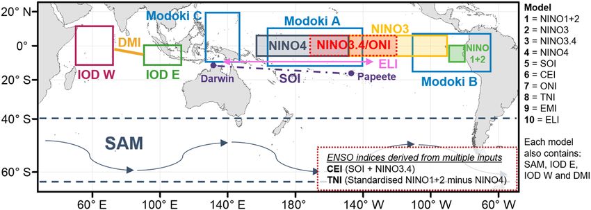
www.nature.com/scientificreports/
Figure 3. Comparison of observed (IBTrACS) TC counts and predicted TC counts for outlooks initialised in
October for the following November–April TC season. 5–95% confidence intervals (CI) for predicted TC counts
are shown in grey. Dashed line represents linear trend of observed (IBTrACS) TC counts.
superior model at least once, highlighting the importance of including multiple ENSO indices to represent the
complex ocean–atmosphere interactions associated with the phenomenon and location-specific o utcomes42,50.
SAM accounts for 11.1% (New Caledonia) to 30.3% (C SWP) of covariates, confirming it is an important climate
mode to consider in order to improve the predictive skill of TC outlook models.
Discussion
We have derived and tested Poisson regression that uses indices representing multiple modes of climate vari-
ability for bespoke island-scale and sub-regional scale TC guidance. This approach can provide up to three
months additional lead time compared to current operational regional TC seasonal outlooks. We tested model
performance across a number of initialisation periods and found that model skill was sufficient to enable TC
count outlooks prior to (from as early as July) and during the early (November–January) SWP TC season (which
is designated by the PINMS as including November–April). In-season monthly TC count outlooks generated
using the method presented here indicates that the later the outlooks are generated, the more accurate they are.
Scientific Reports | (2020) 10:11286 | https://doi.org/10.1038/s41598-020-67646-7 6
Vol:.(1234567890)www.nature.com/scientificreports/
Figure 4. Model overestimate (O) and underestimate (U) time series for TC models initiated in
October according to El Niño, La Niña and Neutral Phases (NINO3.4 Nov–Apr anomalies (1981–2010
climatology); > + 0.5° = El Niño, < 0.5 °C = La Niña, ENSO neutral between + 0.5 °C and − 0.5 °C. O (U) indicates
model has overestimated (underestimated) TC counts compared to IBTrACS observations. Exact strike rate
(SR-E) is the % of time where predicted TCs and observed TCs match between 1970 and 2019. Statistics (%) for
SR-E, O and U are also summarised on each panel.
Compared to other studies that explore various methodologies to derive TC forecasts for the SWP, includ-
ing simple linear regression a pproaches51, Bayesian r egression52, Poisson regression53,54, and machine learning
algorithms45, the method presented in this analysis is unique in a number of ways. First, for each predictor model,
the automated covariate selection algorithm enabled the optimum combination of five Indo-Pacific climate indi-
ces, each of which has six-monthly lags (30 covariates in total). Second, given ENSO is the dominant mode of
variability in the Pacific55, and the well-established ENSO-TC frequency relationship23,29,30, 10 unique predictor
models (each of which contained a unique ENSO index) are tested for each regional, sub-regional and island-
scale location. Superior models were selected using the highest SS (see Data and Model Development). Inclusion
of an extensive range of ENSO indices circumvents issues surrounding subjectivity in choosing an ENSO index,
which has the potential to limit a model’s prediction potential. Third, the results shown in Table 3 show that the
average proportional contribution of indices contained across all regional, sub-regional and island-scale models
Scientific Reports | (2020) 10:11286 | https://doi.org/10.1038/s41598-020-67646-7 7
Vol.:(0123456789)www.nature.com/scientificreports/
Figure 5. Model performance according to month of model initialisation. Models initialised in July–October
predict the entire SWP TC season (November–April). In-season outlooks initialised in November, December
and January, predict TCs for the remaining TC season; December–April, January–April and February–April,
respectively. Numbers above x-axis indicate chosen predictor model due to superior model performance (see
Table 1 for predictor model summary). See Tables S1 and S2 (supplementary material) for more information
regarding model performance according to month of model initialisation.
account for 45.6% (Indian Ocean SST variability; IOD E, IOD W and DMI), 31.9% (ENSO) and 22.5% (SAM).
For every sub-regional/island-scale model and model initialisation period, every ENSO index was used at least
once. While not every mode of tropical and extratropical variability could be included in this analysis, consider-
ing ENSO, SAM and Indian Ocean SST variability and the interactions between them, has proven to add skill
across all regional, sub-regional and island-scale models and initialisation periods.
The benefits of generating independent, location-specific TC outlook models using Poisson regression are
wide-reaching, and not confined to the SWP. They have potential to provide skilful island-scale TC count esti-
mates for each season at a variety of lead times, and this approach can potentially be adapted to other ocean
basins (as well as other time-transgressive geospatial datasets) where multiple driving factors for storm activity
come into play. For the SWP, this new approach provides a complementary perspective to regional outlooks from
official forecasting agencies that only consider how regional TC activity may impact island nations and territories.
Island-scale and sub-regional scale outlooks based on Poisson regression outlooks for TCs also have the potential
to improve testing of storm count strike rates because calibration and verification for this method is undertaken
over a finer spatial scale than what is used for present regional TC outlooks. From this perspective, our new
Scientific Reports | (2020) 10:11286 | https://doi.org/10.1038/s41598-020-67646-7 8
Vol:.(1234567890)www.nature.com/scientificreports/
Subregional models Island-scale models
Solomon
Index SWP C SWP N SWP NE SWP SE SWP Fiji N New Zealand New Caledonia Papua New Guinea Islands Tonga Vanuatu
NINO1 + 2 3.3 0 0 6.3 2.3 7.4 3.8 0 8.0 0 0 5.1
NINO3 0 3.9 0 0 11.5 5.6 0 11.1 14.0 7.7 0 5.1
NINO3.4 0 0 2.8 3.8 0 0 10.3 0 0 4.6 3.5 0
NINO4 6.7 1.3 5.6 0 0 11.1 0 8.9 0 0 3.5 3.4
SOI 0 0 5.6 3.8 9.2 3.7 3.8 0 0 4.6 3.5 0
CEI 0 0 0 6.3 0 5.6 0 0 8.0 0 0 6.8
ONI 0 9.2 0 0 3.4 0 0 8.9 0 0 7.0 0
TNI 13.3 0 19.4 0 0 0 5.1 8.9 0 6.2 0 0
EMI 3.3 14.5 0 0 0 0 3.8 0 0 7.7 10.5 13.6
ELI 5.0 0 0 10.1 0 0 0 0 10.0 0 0 1.7
SAM 23.3 30.3 18.1 24.1 26.4 27.8 26.9 11.1 24.0 20.0 28.1 10.2
IOD E 21.7 17.1 18.1 24.1 27.6 9.3 23.1 22.2 16.0 24.6 19.3 27.1
IOD W 23.3 22.4 26.4 21.5 18.4 29.6 23.1 26.7 20.0 24.6 24.6 27.1
DMI 0 1.3 4.2 0 1.1 0 0 2.2 0 0 0 0
Table 3. Proportion (%) of model covariates for outlook model runs from July–January. Bold values indicates
ENSO index with the largest proportional contribution per location.
approach adds an additional layer of validated guidance relative to extant statistical and dynamical TC outlook
products. In doing so, this addition strengthens the prospect for SWP ensemble-based guidance for TC activity.
The methodology outlined in this paper can also be applied, updated and retrained to incorporate storm
counts from the most recent TC seasons. As such, we expect future improvements for the skill and reduction of
uncertainty for island-scale TC outlooks using this approach. In addition, the ability to easily re-run the models
every month to include the most recent ocean–atmosphere conditions (model covariates), means TC guidance
can be updated on a monthly basis between July and January to cover the SWP TC season that lies ahead. This is
expected to help bridge current sub-seasonal and seasonal climate guidance that indicates where storm activity
may be elevated or reduced, which can change quickly depending on intra-seasonal ENSO developments. This
guidance will be updated and freely available on the Tropical Cyclone Outlook for the Southwest Pacific (TCO-
SP) website (www.tcoutlook.com), to support end-users (including meteorological and government agencies,
civil defence managers, non-governmental aid organisations and the general public) who can access it in sup-
port of decision making and to promote the benefits of expanding early warning systems for weather extremes.
Data and model development
Tropical cyclone data. This study uses TC best-track data from the International Best-Track Archive for
Climate Stewardship (IBTrACSv4)56 for the southwest Pacific (SWP; 0–35°S, 135°E–120°W). The SWP TC sea-
son extends from November to April (the following year). While TCs can occur outside of the SWP TC season,
we only consider events that occur within the SWP TC season. Only events where sustained winds of > 34 kt
(63 km/h) are included in this analysis.
Exclusive Economic Zones (EEZs) are used to delineate island group boundaries. In total, 23 EEZs exist
in the SWP region (Fig. 1a). The number of TCs to pass within each EEZ is calculated on a monthly basis
(Nov–Apr) between 1970 and 2019. Seasonal TC climatologies (Fig. 1a), range from 3.12 TCs per season (Fiji)
to 0.06 TCs per season (C. Kiribati and Marquesas). A threshold of 1.5 TCs per season is used to determine
which EEZ should have an individual outlook model, and which EEZs may suffer from insignificant skill due
to small sample size. Where the seasonal TC climatology < 1.5, geographically neighbouring EEZs are grouped
together (Fig. 1b). Northern New Zealand is an exception as its relative isolation does not allow it to be merged
with another EEZ. Seven individual island-scale outlooks are derived and include Papua New Guinea, Solomon
Islands, New Caledonia, Vanuatu, Fiji, Tonga and Northern New Zealand. Where seasonal TC climatology < 1.5,
four sub-regional EEZ outlooks are derived: northern SWP (N SWP; 1.84 TCs per season), central SWP (C
SWP; 1.8 TCs per season), northeastern SWP (NE SWP; 1.22 TCs per season) and southeastern SWP (SE SWP;
1.92 TCs). The split between the NE SWP and SE SWP was influenced by the average location of the SPCZ, an
important component that influences regional climate57. A model is also derived for the entire SWP basin. The
Gilbert and Phoenix Islands (Kiribati) have not been included in this analysis as these regions are at minimal
risk of TC activity. In total, twelve outlooks are derived and validated in this analysis.
Model covariates. A total of 14 monthly indices representing Indo-Pacific climate variability are used in
this analysis (see Fig. 6). Only one ENSO indicator at a time is paired with indices 2–5 below, resulting in ten
unique predictor models. Further details are outlined below:
1. ENSO: Ten ENSO indices are evaluated in this analysis and include (a) NINO1 + 248, (b) N
INO348, (c)
NINO3.458, (d) N
INO432, (e) Southern Oscillation Index (SOI)33, (f) Coupled ENSO Index (CEI)34, (g)
Scientific Reports | (2020) 10:11286 | https://doi.org/10.1038/s41598-020-67646-7 9
Vol.:(0123456789)www.nature.com/scientificreports/
Figure 6. Indo-Pacific climate indices (model covariates) considered in this analysis. Indices representing El
Niño-Southern Oscillation (ENSO) include: NINO1 + 2, NINO3, NINO4, NINO3.4, Southern Oscillation Index
(SOI), ENSO Modoki Index (EMI), Coupled ENSO Index (CEI), Oceanic Nino Index (ONI), Trans NINO
Index (TNI) and ENSO Longitude Index (ELI). Other indices considered include the Southern Annular Mode
(SAM), Indian Ocean Dipole West pole (IOD W), Indian Ocean Dipole East pole (IOD E), and the Dipole
Mode Index (DMI). Ten predictor model combinations used in analysis are summarised to the right of the panel
and in Table 1. Monthly averaged lags (lag 1–6) are generated for each outlook initiation period. Basemap from
Natural Earth (www.naturalearthdata.com).
Oceanic NINO Index (ONI)35, (h) Trans Nino Index (TNI)48, (i) ENSO Modoki Index (EMI)59, and (j) ENSO
Longitude Index (ELI)36. All oceanic based indices are calculated using E
RSSTv560. In calculating the CEI,
we use a 3-month smoothed version with anomalies calculated using a 1970–2018 climatology. See Fig. 6
for a diagrammatic representation of all indices included for analysis.
2. Marshall SAM Index: a station-based index based on zonal pressure differences between 40°S and 65°S47.
3. IOD E: SST anomalies in the IOD E region (eastern pole of DMI; 0°–10°S, 90°E–110°E38.
4. IOD W: SST anomalies in the IOD W region (western pole of DMI; 10°N–10°S, 50°E–70°E38.
5. DMI: the difference in SST anomalies between IOD W and IOD E 38.
Model development: deriving regional, sub‑regional and island‑scale TC outlooks. Poisson
regression, a special case of generalised linear modelling (GLM) is used to calculate the contribution of model
covariates to predict observed TCs, y, during the training period between 1970 and 2019 (50 seasons in total).
Consistent with other studies44,53,54,61–63, we follow a Poisson distributional process is modelling TC counts given
their discrete nature61. As such,
µy exp(−µi )
P Yi = y = i (1)
, y = 0, 1, 2, . . .
y!
where:
��
(2)
�
µi = expβ0 + βj xij
j
where μi is the expected number of TC counts with covariate values xij for the j predictors on the i th observation.
βj refers to the regression coefficient for each covariate and βo, the intercept.
Prior to variable selection, each predictor model contains six consecutive one-month values (lags). For exam-
ple, models initiated in October will have values from lag 1 (September) through to lag 6 (April) and models
initiated in July, lag 1 is June and lag 6 is January. For each of the 10 predictor models, there are 30 variables (5
indices with 6 monthly lags). Variable selection is used to identify the most appropriate combination of predictors
for each of the ten predictor models per EEZ. Stepwise model selection is performed using the stepAIC function
in the MASS R p ackage64. Forward and backward elimination was used to successively include and/or remove
variables using the AIC (Akaike Information C riterion65) as a selection criterion for choosing when the variable
elimination procedure should stop. Poisson regression is then applied to these selected covariates to derive an
outlook TC timeseries. Checks on the mean–variance relationship over all EEZs and on the total TC count for
lag-1 serial correlation and overdispersion confirmed that Poisson regression was appropriate.
Model validation was then used to evaluate the performance and predictive skill of each model66. Twofold
cross validation is used to evaluate the performance and predictive skill of each model66. Applying twofold cross
validation four times, the 50-year time series is divided into two 25-year blocks and model performance is evalu-
ated. Calibration is performed four times: on the first half (1970–1994), the second half (1995–2019), the middle
half (1982–2006) and on a split between the start (1970–1981) and end (2007–2019) of the time series. Validation
is subsequently performed on the remaining periods. This method of cross-validation evaluates how well the
model performs when trained on only half of the 50-year time series. The selected covariates from the variable
Scientific Reports | (2020) 10:11286 | https://doi.org/10.1038/s41598-020-67646-7 10
Vol:.(1234567890)www.nature.com/scientificreports/
elimination procedure above were the starting point for the training phase to evaluate real-time outlooks skill,
and assesses how well a model is able to replicate decreasing trends in TC counts (see Fig. 3).
The following performance measures were used to evaluate the predictive skill of the TC outlooks compared
to the observations: the Pearson correlation coefficient (predicted TCs versus observed TCs), root mean square
error of the prediction (RMSE), strike rate (SR) exact (SR-exact) (% of time the prediction (rounded to the nearest
whole number) matches the observation) and SR ± 1 (as per exact, but where prediction is ± 1 from observation).
SR ± 1 is sensitive to the mean and variance of TC counts for a given forecast region and is more likely to be
high if the overall mean and variance of TC counts is low. This should be taken into consideration when using
this statistic. Skill score (SS), an evaluation of model performance is also c alculated67, where 100% represents a
perfect outlook and 0% represents outlooks as accurate as the climatology. The finite sample corrected Akaike
information criterion ( AICC) is used to estimate the quality of a model relative to a nother65.
For each island-scale TC outlook, the skill of each of the ten predictor models is evaluated before the best
performing model is selected. Given this study also tests how the skill of TC outlooks change depending on when
the model is initialised, lag 1 is always one month before the model initialisation month. The study completes
the above methodology for each of the 10 predictor models (Table 1) and considers 7 different model initialisa-
tion months (July–January) for each of the 12 regional, sub-regional and island-scale outlooks (840 model runs
in total).
Received: 5 March 2020; Accepted: 11 June 2020
References
1. Bettencourt, S. et al. Not If But When: Adapting to Natural Hazards in the Pacific Islands Region - A Policy Note (English) (World
Bank, Washington, DC, 2006). http://documents.worldbank.org/curated/en/840931468086057665/Not-if-but-when-adapting-
to-natural-hazards-in-the-Pacifi c-Islands-Region-a-policy-note.
2. Terry, J. P., McGree, S. & Raj, R. The exceptional flooding on Vanua Levu Island, Fiji, during Tropical Cyclone Ami in January
2003. J. Nat. Disaster Sci. 26, 27–36 (2004).
3. McInnes, K. L., Grady, J. G. O., Walsh, K. J. E. & Colberg, F. Progress towards quantifying storm surge risk in Fiji due to climate
variability and change. J. Coast. Res. Special Issue 64: Proceedings of the 11th international coastal symposium ICS2011, 1121–1124
(2011).
4. Brown, P., Daigneault, A. & Gawith, D. Climate change and the economic impacts of flooding on Fiji. Clim. Dev. 5529, 1–12 (2016).
5. Barnett, J. Adapting to climate change in Pacific Island countries: the problem of uncertainty. World Dev. 29, 977–993 (2001).
6. Connell, J. Islands at Risk? Environments, Economies and Contemporary Change (Edward Elgar Publishing Limited, Cheltenham,
2013).
7. McKenzie, E., Prasad, B. & Kaloumaira, A. Economic Impact of Natural Disasters on Development in the Pacific: Volume 1 Research
Report (The University of the South Pacific, 2005).
8. Mimura, N. Vulnerability of island countries in the South Pacific to sea level rise and climate change. Clim. Res. 12, 137–143 (1999).
9. Royle, S. A. A Geography of Islands: Small Island Insularity (Taylor & Francis, London, 2002).
10. Mataki, M., Koshy, K. & Nair, V. Implementing Climate Change Adaptation in the Pacific Islands : Adapting to Present Climate Vari-
ability and Extreme Weather Events in Navua (Fiji) (Assessments of Impacts and Adaptations to Climate Change (AIACC), 2006).
11. Nunn, P. D. Vulnerability and adaptive capacity in the archipelagos of the South Pacific. AIACC Asia Regional Workshop Session
C2: Water Resources, Watersheds, Coasts (Bangkok, 26.3.03) (2003).
12. Jones, S. C. et al. The extratropical transition of tropical cyclones: forecast challenges, current understanding, and future directions.
Weather Forecast. 18, 1052–1092 (2003).
13. Lorrey, A. M. et al. An ex-tropical cyclone climatology for Auckland, New Zealand. Int. J. Climatol. 34, 1157–1168 (2014).
14. Nishijima, K. et al. DPRI-VMGD Joint Survey for Cyclone Pam Damages (Port-Vila, Vanuatu, 2015). http://www.taifu.dpri.kyoto
-u.ac.jp/wp-content/uploads/2015/05/DPRI-VMGD-survey-first-report-Final.pdf.
15. Noy, I. Tropical storms: the socio-economics of cyclones. Nat. Clim. Change 6, 343–345 (2016).
16. Terry, J. P. Tropical Cyclones: Climatology and Impacts in the South Pacific (Springer, Berlin, 2007).
17. National Institute for Water and Atmospheric Research (NIWA). Southwest Pacific Tropical Cyclone Outlook—October 2019
(2020). Available at: https://niwa.co.nz/climate/southwest-pacifi c-tropical-cyclone-outlook/southwest-pacifi c-tropical-cyclone-
outlook-october-2019. (Accessed: 5th February 2020).
18. National Institute for Water and Atmospheric Research (NIWA). Island Climate Update (2020). Available at: https://niwa.co.nz/
climate/island-climate-update. (Accessed: 28th February 2020).
19. Kuleshov, Y., Qi, Z., Fawcett, R. & Jones, D. Improving preparedness to natural hazards: Tropical cyclone seasonal prediction for
the southern hemisphere. In Advances in Geosciences: Volume 12: Ocean Science (OS) (ed. Gan, J.) 127–143 (World Scientific, 2008).
https://doi.org/10.1142/9789812836168_0010.
20. Fiji Meteorological Service (FMS). Tropical Cyclone Outlook 2019–20: Regional Specialized Meteorological Centre Nadi Tropical
Cyclone Centre Area of Responsibility. (2020). Available at: https://www.met.gov.fj/index.php?page=tcseasonpro. (Accessed: 5th
February 2020)
21. Zheng, X. T. Indo-pacific climate modes in warming climate: consensus and uncertainty across model projections. Curr. Clim.
Change Rep. 5, 308–321 (2019).
22. Magee, A. D., Verdon-Kidd, D. C., Diamond, H. J. & Kiem, A. S. Influence of ENSO, ENSO Modoki and the IPO on tropical
cyclogenesis: a spatial analysis of the southwest Pacific region. Int. J. Climatol. 37, 1118–1137 (2017).
23. Chand, S. S., McBride, J. L., Tory, K. J., Wheeler, M. C. & Walsh, K. J. E. Impact of different ENSO regimes on southwest Pacific
tropical cyclones. J. Clim. 26, 600–608 (2013).
24. Chattopadhyay, R., Dixit, S. A. & Goswami, B. N. A modal rendition of ENSO diversity. Sci. Rep. 9, 1–11 (2019).
25. Gray, W. M. Tropical Cyclone Genesis. Dept. Atmos. Sci. Colarado State Univ. Fort Collins, CO, 121. Paper No. 120 (1975).
26. Tory, K. J. & Frank, W. M. Tropical cyclone formation. In Global Perspectives on Tropical Cyclones: From Science to Mitigation (eds.
Chan, J. C. L. & Kepert, J. D.) 436 (World Scientific, 2010).
27. Folland, C. K., Renwick, J. A., Salinger, M. J. & Mullan, A. B. Relative influences of the interdecadal Pacific oscillation and ENSO
on the South Pacific Convergence Zone. Geophys. Res. Lett. 29, 2–5 (2002).
28. Vincent, E. M. et al. Interannual variability of the South Pacific Convergence Zone and implications for tropical cyclone genesis.
Clim. Dyn. 36, 1881–1896 (2011).
29. Magee, A. D., Verdon-Kidd, D. C., Diamond, H. J. & Kiem, A. Influence of ENSO, ENSO Modoki and the IPO on tropical cyclo-
genesis: a spatial analysis of the southwest Pacific region. Int. J. Climatol. 37(S1), 1118–1137 (2016).
Scientific Reports | (2020) 10:11286 | https://doi.org/10.1038/s41598-020-67646-7 11
Vol.:(0123456789)www.nature.com/scientificreports/
30. Diamond, H. J., Lorrey, A. M. & Renwick, J. A. A southwest Pacific tropical cyclone climatology and linkages to the El Niño-
southern oscillation. J. Clim. 26, 3–25 (2013).
31. Trenberth, K. E., Stepaniak, D. P. & Smith, L. Interannual variability of patterns of atmospheric mass distribution. J. Clim. 18,
2812–2825 (2005).
32. Glantz, M. Currents of Change: El Niño’s Impact on Climate and Society (Cambridge University Press, Cambridge, 1996).
33. Troup, A. J. The ‘southern oscillation’. Q. J. R. Meteorol. Soc. 91, 490–506 (1965).
34. Gergis, J. L. & Fowler, A. M. Classification of synchronous oceanic and atmospheric El Niño-Southern Oscillation (ENSO) events
for palaeoclimate reconstruction. Int. J. Climatol. 25, 1541–1565 (2005).
35. Kousky, V. E. & Higgins, R. W. An alert classification system for monitoring and assessing the ENSO cycle. Weather Forecast. 22,
353–371 (2007).
36. Williams, I. N. & Patricola, C. M. Diversity of ENSO events unified by convective threshold sea surface temperature: a nonlinear
ENSO index. Geophys. Res. Lett. 45, 9236–9244 (2018).
37. Hanley, D. E., Bourassa, M. A., Brien, J. J. O., Smith, S. R. & Spade, E. R. A quantitative evaluation of ENSO indices. J. Clim. 16(8),
1249–1258 (2002).
38. Saji, N. H., Goswami, B. N., Vinayachandran, P. N. & Yamagata, T. A dipole mode in the tropical Indian Ocean. Nature 401, 360–363
(1999).
39. Liu, K. S. & Chan, J. C. L. Interannual variation of Southern Hemisphere tropical cyclone activity and seasonal forecast of tropical
cyclone number in the Australian region. Int. J. Climatol. 32, 190–202 (2012).
40. Ramsay, H. A., Richman, M. B. & Leslie, L. M. The modulating influence of Indian Ocean sea surface temperatures on Australian
region seasonal tropical cyclone counts. J. Clim. https://doi.org/10.1175/JCLI-D-16-0631.1 (2017).
41. Wijnands, J. S., Shelton, K. & Kuleshov, Y. Improving the operational methodology of tropical cyclone seasonal prediction in the
Australian and the South Pacific Ocean regions. Adv. Meteorol. 2014, 1–8 (2014).
42. Magee, A. D. & Verdon-Kidd, D. C. Indian Ocean sea surface temperature variability, ENSO and tropical cyclogenesis: a spatial
analysis of the southwest Pacific region Int. J. Climatol. 37, 1118–1137 (2017).
43. Diamond, H. J. & Renwick, J. A. The climatological relationship between tropical cyclones in the southwest Pacific and the Southern
Annular Mode. Int. J. Climatol. https://doi.org/10.1002/joc.4007 (2015).
44. Magee, A. D. Verdon-Kidd DC (2019) Historical variability of southwest Pacific tropical cyclone counts since 1855. Geophys. Res.
Lett. 1, 2019GL082900. https://doi.org/10.1029/2019GL082900 (2019).
45. Wijnands, J. S. et al. Seasonal forecasting of tropical cyclone activity in the Australian and the South Pacific Ocean regions. Math.
Clim. Weather Forecast. 1, 21–42 (2015).
46. Flanders Marine Institute. MarineRegions.org. (2020). Available at: www.marineregions.org. (Accessed: 10th January 2020).
47. Marshall, G. Trends in the southern annular mode from observations and reanalyses. J. Clim. 16(24), 4134–4143 (2003).
48. Trenberth, K. & Stepaniak, D. Indices of El Niño evolution. J. Clim. 14(8), 1697–1701 (2001).
49. Magee, A. D., Verdon-Kidd, D. C. & Kiem, A. S. An intercomparison of tropical cyclone best-track products for the southwest
Pacific. Nat. Hazards Earth Syst. Sci. 16, 1431–1447 (2016).
50. Kiem, A. S. & Franks, S. W. On the identification of ENSO-induced rainfall and runoff variability: a comparison of methods and
indices. Hydrol. Sci. J. 46, 715–727 (2001).
51. Nicholls, N. SOI-based forecast of Australian region tropical cyclone activity. Exp. Long Lead Forecast. Bull. 8, 71–72 (1999).
52. Chand, S. S., Walsh, K. J. E. & Chan, J. C. L. A bayesian regression approach to seasonal prediction of tropical cyclones affecting
the Fiji region. J. Clim. 23, 3425–3445 (2010).
53. McDonnell, K. A. & Holbrook, N. J. A Poisson regression model approach to predicting tropical cyclogenesis in the Australian/
southwest Pacific Ocean region using the SOI and saturated equivalent potential temperature gradient as predictors. Geophys. Res.
Lett. 31, 1–5 (2004).
54. McDonnell, K. A. & Holbrook, N. J. A poisson regression model of tropical cyclogenesis for the Australian-southwest Pacific Ocean
region. Weather Forecast. 19, 440–455 (2004).
55. Trenberth, K. E. The definition of El Niño. Bull. Am. Meteorol. Soc. 78, 2771–2777 (1997).
56. Knapp, K. R., Diamond, H. J., Kossin, J. P., Kruk, M. C. & Schreck, C. J. International Best Track Archive for Climate Stewardship
(IBTrACS) Project, Version 4. NOAA National Centers for Environmental Information (2018). Available at: https: //doi.org/10.25921
/82ty-9e16. (Accessed: 2nd October 2019).
57. Lorrey, A., Dalu, G., Renwick, J., Diamond, H. & Gaetani, M. Reconstructing the south Pacific convergence zone position during
the Presatellite Era: A La Niña case study. Mon. Weather Rev. 140, 3653–3668 (2012).
58. Barnston, A. G., Chelliah, M. & Goldenberg, S. B. Documentation of a highly ENSO-related SST region in the equatorial pacific.
Atmos. Ocean 35, 367–383 (1997).
59. Kim, H. M., Webster, P. J. & Curry, J. A. Modulation of North Pacific tropical cyclone activity by three phases of ENSO. J. Clim.
24, 1839–1849 (2011).
60. Huang, B. et al. Extended reconstructed Sea surface temperature, Version 5 (ERSSTv5): upgrades, validations, and intercompari-
sons. J. Clim. 30, 8179–8205 (2017).
61. Elsner, J. B. & Schmertmann, C. P. Improving extended-range seasonal predictions of intense Atlantic hurricane activity. Weather
Forecast. 8, 345–351 (1993).
62. Mann, M. E., Sabbatelli, T. A. & Neu, U. Evidence for a modest undercount bias in early historical Atlantic tropical cyclone counts.
Geophys. Res. Lett. 34, 1–6 (2007).
63. Sabbatelli, T. A. & Mann, M. E. The influence of climate state variables on Atlantic tropical cyclone occurrence rates. J. Geophys.
Res. Atmos. 112, 1–8 (2007).
64. Ripley, B. et al. Package ‘MASS’. Cran R (2019). Available at: https://www.stats.ox.ac.uk/pub/MASS4/. (Accessed: 7th February
2020).
65. Burnham, K. P. & Anderson, D. R. Multimodel inference: understanding AIC and BIC in model selection. Sociol. Methods Res. 33,
261–304 (2004).
66. Wilks, D. S. Statistical Methods in the Atmospheric Sciences (Academic Press, London, 2011).
67. Roebber, P. J. & Bosart, L. F. The complex relationship between forecast skill and forecast value: a real-world analysis. Weather
Forecast. 11, 544–559 (1996).
Author contributions
A.D.M. conceived of the presented idea with input from A.M.L. and A.S.K.. A.D.M. developed the theory and was
assisted by K.C. to generate the code. All authors verified the analytical methods. A.D.M. wrote the manuscript in
consultation with A.M.L., A.S.K. and K.C. All authors discussed the results and commented on the manuscript.
Competing interests
The authors declare no competing interests.
Scientific Reports | (2020) 10:11286 | https://doi.org/10.1038/s41598-020-67646-7 12
Vol:.(1234567890)www.nature.com/scientificreports/
Additional information
Supplementary information is available for this paper at https://doi.org/10.1038/s41598-020-67646-7.
Correspondence and requests for materials should be addressed to A.D.M.
Reprints and permissions information is available at www.nature.com/reprints.
Publisher’s note Springer Nature remains neutral with regard to jurisdictional claims in published maps and
institutional affiliations.
Open Access This article is licensed under a Creative Commons Attribution 4.0 International
License, which permits use, sharing, adaptation, distribution and reproduction in any medium or
format, as long as you give appropriate credit to the original author(s) and the source, provide a link to the
Creative Commons licence, and indicate if changes were made. The images or other third party material in this
article are included in the article’s Creative Commons licence, unless indicated otherwise in a credit line to the
material. If material is not included in the article’s Creative Commons licence and your intended use is not
permitted by statutory regulation or exceeds the permitted use, you will need to obtain permission directly from
the copyright holder. To view a copy of this licence, visit http://creativecommons.org/licenses/by/4.0/.
© The Author(s) 2020
Scientific Reports | (2020) 10:11286 | https://doi.org/10.1038/s41598-020-67646-7 13
Vol.:(0123456789)You can also read