A Random Forests Approach to Predicting Clean Energy Stock Prices
←
→
Page content transcription
If your browser does not render page correctly, please read the page content below
Journal of
               Risk and Financial
               Management

Article
A Random Forests Approach to Predicting Clean Energy
Stock Prices
Perry Sadorsky

                                          Schulich School of Business, York University, Toronto, ON M3J 1P3, Canada; psadorsky@schulich.yorku.ca

                                          Abstract: Climate change, green consumers, energy security, fossil fuel divestment, and technological
                                          innovation are powerful forces shaping an increased interest towards investing in companies that
                                          specialize in clean energy. Well informed investors need reliable methods for predicting the stock
                                          prices of clean energy companies. While the existing literature on forecasting stock prices shows
                                          how difficult it is to predict stock prices, there is evidence that predicting stock price direction is
                                          more successful than predicting actual stock prices. This paper uses the machine learning method
                                          of random forests to predict the stock price direction of clean energy exchange traded funds. Some
                                          well-known technical indicators are used as features. Decision tree bagging and random forests
                                          predictions of stock price direction are more accurate than those obtained from logit models. For a
                                          20-day forecast horizon, tree bagging and random forests methods produce accuracy rates of between
                                          85% and 90% while logit models produce accuracy rates of between 55% and 60%. Tree bagging and
                                          random forests are easy to understand and estimate and are useful methods for forecasting the stock
                                          price direction of clean energy stocks.

                                          Keywords: clean energy stock prices; forecasting; machine learning; random forests


Citation: Sadorsky, Perry. 2021. A
                                          1. Introduction
Random Forests Approach to
Predicting Clean Energy Stock Prices.          Climate change, green consumers, energy security, fossil fuel divestment, and tech-
Journal of Risk and Financial             nological innovation are powerful forces shaping an increased interest towards investing
Management 14: 48. https://doi.org/       in companies that specialize in clean energy, broadly defined as energy produced from re-
10.3390/jrfm14020048                      newable energy sources like biomass, geothermal, hydro, wind, wave, and solar. Through
                                          technological innovation, the levelized cost of electricity is falling for renewables and
Academic Editor: Jong-Min Kim             onshore wind is now less costly than coal (The Economist 2020). Investment in clean
Received: 31 December 2020                energy equities totaled $6.6 billion in 2019. While this number was below the record
Accepted: 21 January 2021                 high of $19.7 billion in 2017, the compound annual growth rate between 2004 and 2019 of
Published: 24 January 2021                24% was above that of clean energy private equity or venture capital funding (Frankfurt
                                          School-UNEP Centre/BNEF 2020).
Publisher’s Note: MDPI stays neutral           Well informed investors need reliable methods for predicting the stock prices of clean
with regard to jurisdictional claims in   energy companies. There is, however, a noticeable lack of information on the prediction of
published maps and institutional affil-   clean energy stock prices. This is the gap in the literature that this paper fills. There are,
iations.
                                          however, two complicating issues. First, predicting stock prices is fraught with difficulty
                                          and the prevailing wisdom in most academic circles, consistent with the efficient markets
                                          hypothesis, has generally been that stock prices are unpredictable (Malkiel 2003). More
                                          recently, momentum and economic or psychology behavior factors have been identified
Copyright: © 2021 by the author.          as possible sources of stock price predictability (Gray and Vogel 2016; Lo et al. 2000;
Licensee MDPI, Basel, Switzerland.        Christoffersen and Diebold 2006; Moskowitz et al. 2012). In addition, the existing literature
This article is an open access article    on stock price predictability shows that predicting stock price direction is more successful
distributed under the terms and           than predicting actual stock prices (Basak et al. 2019; Leung et al. 2000; Nyberg 2011;
conditions of the Creative Commons
                                          Nyberg and Pönkä 2016; Pönkä 2016; Ballings et al. 2015; Lohrmann and Luukka 2019).
Attribution (CC BY) license (https://
                                               Second, regression based approaches for predicting stock prices or approaches relying
creativecommons.org/licenses/by/
                                          solely on technical indicators provides mixed results (Park and Irwin 2007) but machine
4.0/).

J. Risk Financial Manag. 2021, 14, 48. https://doi.org/10.3390/jrfm14020048                                    https://www.mdpi.com/journal/jrfm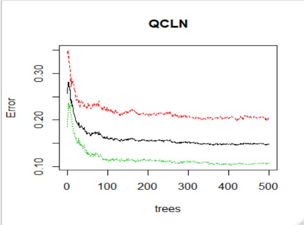
J. Risk Financial Manag. 2021, 14, 48                                                                                            2 of 20

                                        learning (ML) methods appear to offer better accuracy (Shah et al. 2019; Ghoddusi et al.
                                        2019; Khan et al. 2020; Atsalakis and Valavanis 2009; Henrique et al. 2019). There are many
                                        different types of ML methods but decision tree bagging and random forests (RFs) are easy
                                        to understand and motivate and they also tend to have good performance for predicting
                                        stock prices (Basak et al. 2019; Khan et al. 2020; Lohrmann and Luukka 2019). Decision
                                        trees are a nonparametric supervised leaning method for classification and regression.
                                        A decision tree classifier works by using decision rules on the data set features (predictors or
                                        explanatory variables) to predict a target variable (James et al. 2013). Decision trees are easy
                                        to understand and visualize and work on numerical and categorical data (Mullainathan
                                        and Spiess 2017). Decision tree learning can, however, create complicated trees the results
                                        of which are susceptible to small changes in data. Bootstrap aggregation, or bagging as
                                        it is commonly known as, is one way to reduce the variance of decision trees. Bootstrap
                                        replication is used to create many bootstrap training data sets. Even though each tree
                                        is grown deep and has high variance, averaging the predictions from these bootstrap
                                        trees reduces variance. RFs are ensembles of decision trees and work by introducing
                                        decorrelation between the trees by randomly selecting a small set of predictors at each split
                                        of the tree (James et al. 2013).
                                               Here are some recent examples of papers that use RFs for stock price prediction.
                                        Ampomah et al. (2020) compare the performance of several tree-based ensemble methods
                                        (RFs, XGBoost, Bagging, AdaBoost, Extra Trees, and Voting Classifier) in predicting the
                                        direction of stock price change for data from three US stock exchanges. The accuracy
                                        for each model was good and ranged between 82% and 90%. The Extra Trees method
                                        produced the highest accuracy on average. Ballings et al. (2015) point out that among
                                        papers that predict stock price direction with machine learning methods, artificial neural
                                        networks (ANNs) and support vector machines (SVMs) are more popular than RFs. Only
                                        3 out of the 33 papers that they survey used RFs. It is not clear why more complicated
                                        methods like ANN and SVM are preferred over simpler methods like RFs. Using data
                                        on 5767 European listed companies, they compare the stock price direction predictive
                                        performance of RFs, SVMs, AdaBoost, ANNs, K-nearest neighbor and logistic regression.
                                        Feature selection is based on company specific fundamental data. They find strong evidence
                                        that ensemble methods like RFs have greater prediction accuracy over a one-year prediction
                                        period. Basak et al. (2019) use RFs to predict stock price direction for 10 companies, most of
                                        which are technology or social media oriented (AAPL, AMZN, FB, MSFT, TWTR). Feature
                                        selection is based on technical indicators. They find the predictive accuracy of RFs and
                                        XGBoost to be higher than that of artificial neural networks, support vector machines,
                                        and logit models. Khan et al. (2020) use 12 machine learning methods applied to social
                                        media and financial data to predict stock prices (3 stock exchanges and 8 US technology
                                        companies). The RFs method is consistently ranked as one of the best methods. Lohrmann
                                        and Luukka (2019) use RFs to predict the classification of S & P 500 stocks. Stock price
                                        direction is based on a four-class structure that depends upon the difference between the
                                        open and close stock prices. Feature selection is based on technical indicators. They find
                                        that the RFs classifier produces better trading strategies than a buy and hold strategy.
                                        Mallqui and Fernandes (2019) find that a combination of recurrent neural networks and a
                                        tree classifier to be better at predicting Bitcoin price direction than SVM. Mokoaleli-Mokoteli
                                        et al. (2019) study how several ML ensemble methods like boosted, bagged, RUS-boosted,
                                        subspace disc, and subspace k-nearest neighbor (KNN) compare in predicting the stock
                                        price direction of the Johannesburg Stock Exchange. They find that Boosted methods
                                        outperform KNN, logistic regression, and SVM. Nti et al. (2020) also find that RFs tend
                                        to be underutilized in studies that focus on stock price prediction. Weng et al. (2018)
                                        use machine learning methods (boosted regression tree, RFs, ANN, SVM) combined with
                                        social media type data like web page views, financial news sentiment, and search trends to
                                        predict stock prices. Twenty large US companies are studied. RFs and boosted regression
                                        trees outperform ANN or SVM. The main message from these papers is that RFs have high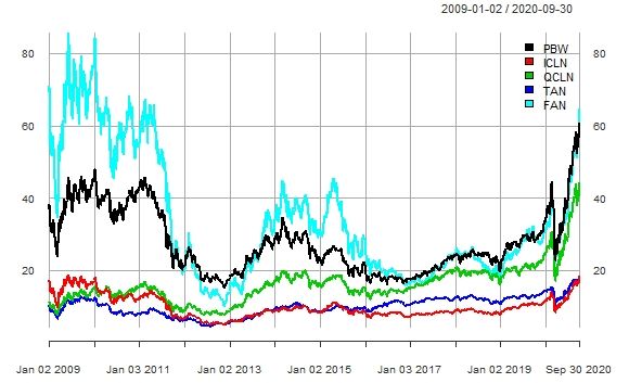
J. Risk Financial Manag. 2021, 14, 48                                                                                               3 of 20

                                        accuracy when predicting stock price direction but are underrepresented in the literature
                                        compared to other machine learning methods.
                                             The purpose of this paper is to predict clean energy stock price direction using random
                                        forests. Directional stock price forecasts are constructed from one day to twenty days in
                                        the future. A multi-step forecast horizon is used in order to gain an understanding of
                                        how forecast accuracy changes across time (Basak et al. 2019; Khan et al. 2020). A five-
                                        day forecast horizon corresponds to one week of trading days, a 10-day forecast horizon
                                        corresponds to two weeks of trading days and a twenty-day forecast horizon corresponds
                                        to approximately one month of trading days. Forecasting stock price direction over a
                                        multi-day horizon provides a more challenging environment to compare models. Clean
                                        energy stock prices are measured using several well-known and actively traded exchange
                                        traded funds (ETFs). Forecasts are constructed using logit models, bagging decision
                                        trees, and RFs. A comparison is made between the forecasting accuracy of these models.
                                        Feature selection is based on several well-known technical indicators like moving average,
                                        stochastic oscillator, rate of price change, MACD, RSI, and advance decline line (Bustos
                                        and Pomares-Quimbaya 2020).
                                             The analysis from this research provides some interesting results. RFs and tree bag-
                                        ging show much better stock price prediction accuracy than logit or step-wise logit. The
                                        prediction accuracy from bagging and RFs is very similar indicating that either method is
                                        very useful for predicting the stock price direction of clean energy ETFs. The prediction
                                        accuracy for RF and tree bagging models is over 80% for forecast horizons of 10 days or
                                        more. For a 20-day forecast horizon, tree bagging and random forests methods produce
                                        accuracy rates of between 85% and 90% while logit models produce accuracy rates of
                                        between 55% and 60%.
                                             This paper is organized as follows. The next section sets out the methods and data.
                                        This is followed by the results and a discussion. The last section of the paper provides
                                        some conclusions and suggestions for future research.

                                        2. Methods and Data
                                        2.1. The Logit Method for Prediction
                                             The objective of this paper is to predict the stock price direction of clean energy stocks.
                                        Stock price direction can be classified as either up (stock price change from one period to the
                                        next is positive) or down (stock price change from one period to the next is non-positive).
                                        This is a standard classification problem where the variable of interest can take on one of
                                        two values (up, down) and is easily coded as a binary variable. One approach to modelling
                                        and forecasting the direction of stock prices is to use logit models. Explanatory variables
                                        deemed relevant to predicting stock price direction can be used as features. Logit models
                                        are widely used and easy to estimate.

                                                                               yt+h = α + βXt + εt ,                                   (1)

                                              In Equation (1), yt+h = pt+h – pt is a binary variable that takes on the value of “up” if
                                        positive or “down” if non-positive and X is a vector of features. The variable pt represents
                                        the adjusted closing stock price on day t. The random error term is ε. The value of h = 1,
                                        2, 3, . . . , 20 indicates the number of time periods into the future to predict. A multistep
                                        forecast horizon is used in order to see how forecast accuracy changes across the forecast
                                        horizon. A 20-day forecast horizon is used in this paper since this is consistent with the
                                        average number of trading days in a month. The features include well-known technical
                                        indicators like the relative strength indicator (RSI), stochastic oscillator (slow, fast), advance-
                                        decline line (ADX), moving average cross-over divergence (MACD), price rate of change
                                        (ROC), on balance volume (OBV), and the 200-day moving average. While there are many
                                        different technical indicators the ones chosen in this paper are widely used in academics
                                        and practice (Yin and Yang 2016; Yin et al. 2017; Neely et al. 2014; Wang et al. 2020; Bustos
                                        and Pomares-Quimbaya 2020).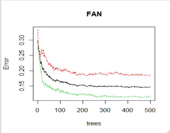
J. Risk Financial Manag. 2021, 14, 48                                                                                              4 of 20

                                        2.2. The Random Forests Method for Prediction
                                             Logit regression classifies the dependent (response) variable based on a linear boundary
                                        and this can be limiting in situations where there is a nonlinear relationship between the
                                        response and the features. In such situations, a decision tree approach may be more useful.
                                        Decision trees bisect the predictor space into smaller and smaller non-overlapping regions
                                        and are better able to capture the classification between the response and the features in
                                        nonlinear situations. The rules used to split the predictor space can be summarized in a tree
                                        diagram, and this approach is known as a decision tree method. Tree based methods are easy
                                        to interpret but are not as competitive with other methods like bagging or random forests.
                                        A brief discussion of decision trees, bagging, and random forest methods is presented here
                                        but the reader is referred to James et al. (2013) for a more complete treatment.
                                             A classification tree is used to predict a qualitative response rather than a quantitative
                                        one. A classification tree predicts that each observation belongs to the most commonly
                                        occurring class of training observations in the region to which it belongs. A majority
                                        voting rule is used for classification. The basic steps in building a classification tree can be
                                        described as follows.
                                        1.   Divide the predictor space (all possible values for X1 , . . . , XP ) into J distinctive and
                                             non-overlapping regions, R1 , . . . , RJ .
                                        2.   For every observation that falls into the region Rj, the same prediction is made. This
                                             prediction is that each observation belongs to the most commonly occurring class of
                                             training observations to which it belongs.
                                             The regions R1 , . . . , RJ can be constructed as follows. Recursive binary splitting is
                                        used to grow the tree and splitting rules are determined by a classification error rate. The
                                        classification error rate, E, is the fraction of training observations in a region that do not
                                        belong to the most common class.

                                                                                          max( p̂mk )
                                                                             E = 1−                                                   (2)
                                                                                             k
                                             In Equation (2), p̂mk is the proportion of training observations in the mth region that
                                        are from the kth class. The classification error is not very sensitive to the growing of trees
                                        so in practice either the Gini index (G) or entropy (D) is used to classify splits.

                                                                                  K
                                                                            G=   ∑ p̂mk (1 − p̂mk )                                   (3)
                                                                                 k =1

                                             The Gini index measures total variance across the K classes. In this paper, there are
                                        only two classes (stock price direction positive, or not) so K = 2. For small values of p̂mk
                                        the Gini index takes on a small value. For this reason, G is often referred to as a measure
                                        of node impurity since a small G value shows that a node mostly contains observations
                                        from a single class. The root node at the top of a decision tree can be found by trying every
                                        possible split of the predictor space and choosing the split that reduces the impurity as
                                        much as possible (has the highest gain in the Gini index). Successive nodes can be found
                                        using the same process and this is how recursive binary splitting is evaluated.

                                                                                      K
                                                                           D=−     ∑ p̂mk log( p̂mk )                                 (4)
                                                                                   k =1

                                              The entropy (D), like the Gini index, will take on small values if the mth node is pure.
                                        The Gini index and entropy produce numerically similar values. The analysis in this paper
                                        uses the entropy measure.
                                              The outcome of this decision tree building process is typically a very deep and complex
                                        tree that may produce good predictions on the training data set but is likely to over fit the
                                        data leading to poor performance on unseen data. Decision trees suffer from high variance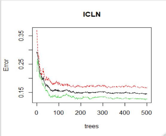
J. Risk Financial Manag. 2021, 14, 48                                                                                           5 of 20

                                        which means that if the training data set is split into two parts at random and a decision
                                        tree fit to both halves, the outcome would be very different. One approach to remedying
                                        this is to use bagging. Bootstrap aggregation or bagging is a statistical technique used to
                                        reduce the variance of a machine learning method. The idea behind bagging it to take many
                                        training sets, build a decision tree on each training data set, and average the predictions to
                                        obtain a single low-variance machine learning model. In general, however, the researcher
                                        does not have access to many training sets so instead bootstrap replication is used to create
                                        many bootstrap training data sets and a decision tree grown for each replication. Each
                                        individual tree is constructed by randomly sampling the predictors with replacements. So,
                                        for example, if the number of predictors is 6, then each tree has 6 predictors but because
                                        sampling is done with replacement some predictors may be sampled more than once. Thus,
                                        the number of bootstrap replications is the number of trees. Even though each tree is
                                        grown deep and has high variance, averaging the predictions from these bootstrap trees
                                        reduces variance. The test error of a bagged model can be easily estimated using the out
                                        of bag (OOB) error. In bagging, decision trees are repeatedly fit to bootstrapped subsets
                                        of the observations. On average, each bagged tree uses approximately two-thirds of the
                                        observations (James et al. 2013). The remaining one-third of the observations not used are
                                        referred to as the OOB observations and can be used as a test data set to evaluate prediction
                                        accuracy. The OOB test error can be averaged across trees.
                                              Random forests are comprised of a large number of individual decision trees that
                                        operate as an ensemble (Breiman 2001). Random forests are non-metric classifiers because
                                        no learning parameters need to be set. Random forests are an improvement over bagging
                                        trees by introducing decorrelation between the trees. As in the case of bagging, a large
                                        number of decision trees are built on bootstrapped training samples. Each individual tree
                                        in the random forest produces a prediction for the class and the class with the most votes is
                                        the model’s prediction. Each time a split in a tree occurs a random sample of predictors
                                        is chosen as split candidates from the full set of predictors. Notice how this differs from
                                        bagging. In bagging all predictors are used at each split. In random forests, the number of
                                        predictors chosen at random is usually calculated as the square root of the total number of
                                        predictors (James et al. 2013). While the choice of randomly choosing predictors may seem
                                        strange, averaging results from non-correlated trees is much better for reducing variance
                                        than averaging trees that are highly correlated. In random forests, trees are trained on
                                        different samples due to bagging and also use different features when predicting outcomes.
                                              This paper compares the performance of logit, step-wise logit, bagging decision tree,
                                        and random forests for predicting the stock price direction of clean energy ETFs. For the
                                        analysis, 80% of the data was used for training and 20% used for testing. Classification
                                        prediction is one of the main goals of classification trees and the accuracy of prediction can
                                        be obtained from the confusion matrix. The logit model uses all of the features in predicting
                                        stock price direction. The step-wise logit uses a backwards step-wise reduction algorithm
                                        evaluated using Akaike Information Criteria (AIC) to create a sub-set of influential features.
                                        The bagging decision tree model was estimated with 500 trees. The random forecasts were
                                        estimated with 500 trees and 3 (the floor of the square root of the number of predictor
                                        variables, 10) randomly chosen predictors at each split (Breiman 2001). The results are
                                        not sensitive to the number of trees provided a large enough number of trees are chosen.
                                        A very large number of trees does not lead to overfitting, but a small number of trees results
                                        in high test error. Training control for the random forest was handled with 10-fold cross
                                        validation with 10 repeats. All calculations were done in R (R Core Team 2019) and used
                                        the random forests machine learning package (Breiman et al. 2018).

                                        2.3. The Data
                                            The data for this study consists of the stock prices of five popular, US listed, and
                                        widely traded clean energy ETFs. The Invesco WilderHill Clean Energy ETF (PBW) is
                                        the most widely known clean energy ETF and has the longest trading period with an
                                        inception date of 3 March 2005. This ETF consists of publicly traded US companies that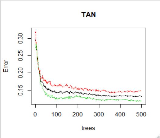
2.3. The Data
The data for this study consists of the stock prices of five popular, US listed, and
widely traded clean energy ETFs. The Invesco WilderHill Clean Energy ETF (PBW) is the
J. Risk Financial Manag. 2021, 14, 48 most widely known clean energy ETF and has the longest trading period with an incep- 6 of 20
tion date of 3 March 2005. This ETF consists of publicly traded US companies that are in
the clean energy business (renewable energy, energy storage, energy conversion, power
delivery, greener utilities, cleaner fuels). The iShares Global Clean Energy ETF (ICLN)
are in the clean energy business (renewable energy, energy storage, energy conversion,
seeks to track the S&P Global Clean Energy Index. The First Trust NASDAQ Clean Edge
power delivery, greener utilities, cleaner fuels). The iShares Global Clean Energy ETF
Green Energy Index Fund (QCLN) tracks the NASDAQ Clean Edge Energy Index. The
(ICLN) seeks to track the S&P Global Clean Energy Index. The First Trust NASDAQ Clean
Invesco Solar ETF (TAN) tracks the MAC Global Solar Energy Index which focuses on
Edge Green Energy Index Fund (QCLN) tracks the NASDAQ Clean Edge Energy Index.
companies that generate a significant amount of their revenue from solar equipment man-
The Invesco Solar ETF (TAN) tracks the MAC Global Solar Energy Index which focuses
ufacturing
on companies or enabling products
that generate for the solar
a significant powerofindustry.
amount The First
their revenue from Trust Global
solar Wind
equipment
Energy ETF (FAN)
manufacturing tracks the
or enabling ISE Clean
products forEdge Global
the solar powerWind EnergyThe
industry. Index and
First consists
Trust Global of
companies throughout the world that are in the wind energy
Wind Energy ETF (FAN) tracks the ISE Clean Edge Global Wind Energy Index and consists industry. TAN and FAN
began trading throughout
of companies near the middle of 2008.
the world thatTheare daily
in the data
windset startsindustry.
energy on January TAN 1, and
2009FAN and
ends on September 30, 2020. The data was collected from Yahoo
began trading near the middle of 2008. The daily data set starts on 1 January 2009 and endsFinance. Several well-
known technical indicators
on 30 September like the
2020. The data wasrelative
collectedstrength indicator
from Yahoo (RSI), Several
Finance. stochastic oscillator
well-known
(slow, fast),
technical advance-decline
indicators like the line (ADX),
relative moving
strength average(RSI),
indicator cross-over divergence
stochastic (MACD),
oscillator (slow,
price rate of change (ROC), on balance volume, and the 200-day
fast), advance-decline line (ADX), moving average cross-over divergence (MACD), price moving average, calcu-
lated
rate offrom daily(ROC),
change data, are
on used
balanceas features
volume,inand the the
logit200-day
and RFsmoving
prediction models.
average, calculated
The time series pattern of the clean energy ETFs shows
from daily data, are used as features in the logit and RFs prediction models. that the ETFs move together
(Figure
The 1).time
There waspattern
series a double ofpeak formation
the clean energyin ETFs
early shows
2009 and that2011
thefollowed
ETFs move by atogether
trough
in 2013. 1).
(Figure This waswas
There followed by peak
a double a peak in 2014 and
formation then2009
in early a relatively
and 2011horizontal
followed by pattern
a troughbe-
tween
in 2013.2017Thisandwas
2019. In response
followed by atopeak
the global
in 2014financial
and then crisis of 2008–2009
a relatively some countries,
horizontal pattern
like the US,
between 2017China, and In
and 2019. South Korea,
response to implemented
the global financial fiscal crisis
stimulus packagessome
of 2008–2009 where the
coun-
economic stimulus
tries, like the was directed
US, China, and South at achieving economic growth
Korea, implemented and environmental
fiscal stimulus packages where sus-
tainability
the economic (Andreoni
stimulus 2020;
wasMundaca
directed and Luth Richter
at achieving 2015).growth
economic This helped to increase the
and environmental
stock prices of(Andreoni
sustainability clean energy companies.
2020; Mundaca and All of the ETFs
Richter 2015). have
Thisrisen sharply
helped since the
to increase the onset
stock
of the World
prices of cleanHealth
energyOrganization’s
companies. All declaration
of the ETFsofhave the COVID19
risen sharplyglobal pandemic
since the onset(March
of the
2020).
World Health Organization’s declaration of the COVID19 global pandemic (March 2020).
Figure 1.
Figure This figure
1. This figure shows
shows clean
clean energy
energy ETF
ETF stock
stock prices
prices across
across time.
time. Data
Data sourced
sourced from
from Yahoo
Yahoo Finance.
Finance.
The histograms for the percentage of up days shows little variation for PBW, ICLN,
and TAN (Figure 2). The percentage of up days increases with the number of days for
QCLN while for FAN, the pattern increases up to about 7 days after which the percentage
of up days shows little variation with longer time periods. Compared to the other clean
energy ETFs studied in this paper, QCLN has the strongest trend in the data (Figure 1) and
this is consistent with the higher proportion of up days.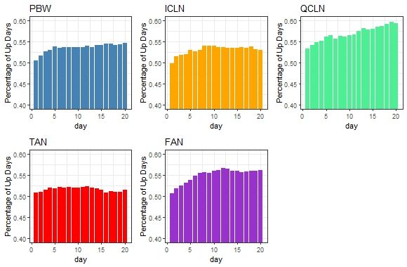
The histograms for the percentage of up days shows little variation for PBW, ICLN,
and TAN (Figure 2). The percentage of up days increases with the number of days for
QCLN while for FAN, the pattern increases up to about 7 days after which the percentage
J. Risk Financial Manag. 2021, 14, 48
of up days shows little variation with longer time periods. Compared to the other clean
7 of 20
energy ETFs studied in this paper, QCLN has the strongest trend in the data (Figure 1)
and this is consistent with the higher proportion of up days.
Figure 2. This
This figure
figure shows
shows histograms
histograms of
of clean
clean energy
energy ETF
ETF percentage
percentage of
of up
up days.
days. Data
Datasourced
sourcedfrom
fromYahoo
Yahoo Finance.
Finance.
Author’s own calculations.
Author’s own calculations.
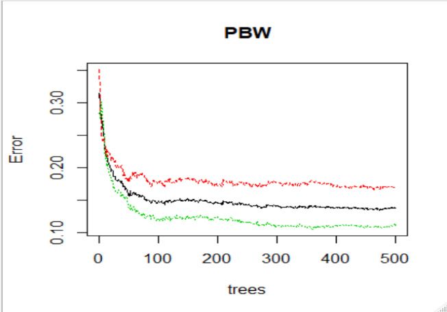
In order
In order totoinvestigate
investigate the
the impact
impact ofofthe
thenumber
numberof oftrees
treeson onthe
therandom
randomforests
forestsmodel,
model,
Figure 3 shows how the test error relates to the number of trees. The analysis
Figure 3 shows how the test error relates to the number of trees. The analysis is conducted is conducted
for aa 10-step
for 10-step forecast
forecast horizon
horizon where
where 80%
80% of of the
the data
data is
is used
used forfor training
training andand 20%20% ofof the
data is
data is used
used for
for testing.
testing. In
In each
each case,
case, the
the test
test error
error declines
declines rapidly
rapidly asas the
the number
number of trees
increases from 1 to
increases to 100.
100. After
After300
300trees
trees there
there isisvery
verysmall
small reduction
reduction in in the
the test
test error.
error. Notice
Notice
how the
how the test
test error
error converges.
converges. This
This shows
shows thatthat random
random forests
forests dodo not
not over
over fit
fit as
as the
the number
number
of trees
of trees increases.
increases. InIn Figure
Figure 3,3, out
out of
of bag
bag (OOB)
(OOB) test
test error
error is
is reported
reported along
along with
with test
test error
error
J. Risk Financial Manag. 2021, 14, x FOR PEER
for the REVIEW
up and down classification. The results for other forecast horizons are 8 of 21
similar to
for the up and down classification. The results for other forecast horizons are similar to
those reported here. Consequently, 500 trees are used in estimating
those reported here. Consequently, 500 trees are used in estimating the RFs. the RFs.
Figure 3. Cont.
J. Risk Financial Manag. 2021, 14, 48 8 of 20
Figure
Figure3.3. This
This figure
figure shows
shows RFs
RFs test
test error
errorvs.
vs. the
the number
number ofof trees.
trees. OOB
OOB (red),
(red), down
down classification
classification (black),
(black), up
up classification
classification
(green).
(green). Calculations
Calculationsare aredone
donefor
forpredicting
predictingstock
stockprice
pricedirection
directionover
overaa10-step
10-stepforecast
forecasthorizon.
horizon.
3. Results
3.
This section
This section reports
reports thethe results
results from
from predicting
predicting stock
stock price
price direction
direction for
for clean
clean energy
energy
ETFs.
ETFs. Since this is a classification problem,
problem, thethe prediction
prediction accuracy
accuracy isis probably
probably thethe single
single
most
most useful measure of forecast performance. Prediction accuracy a proportion of the
useful measure of forecast performance. Prediction accuracy is a proportion of the
number
number of true true positives
positives and true negatives
negatives divided by the total number of predictions.
This
This measure
measure cancan be
be obtained
obtained from from the
theconfusion
confusion matrix.
matrix. Other
Other useful
useful forecast
forecast accuracy
accuracy
measures
measures likelike how
how well
well the
the models
models predict
predict the
the up up or
or down
down classification
classification are
are also
also available
available
and
and are
are reported
reported since
since itit is
is interesting
interesting to
to see
see ifif the
the forecast
forecast accuracy
accuracy for
for predicting
predicting thethe up
up
class is similar or different to that of predicting the
class is similar or different to that of predicting the down class.down class.
Stock price direction prediction accuracy for PWB (Figure 4) shows large differences
between the logit models and RF or logit models and tree bagging. The prediction accuracy
for logit and logit stepwise show that while there is some improvement in accuracy between
1 and 5 days ahead, the prediction accuracy never gets above 0.6 (60%). The prediction
accuracy of the RFs and tree bagging methods show considerable improvement in accuracy
between 1 and 10 days. Prediction accuracy for predicting stock price direction 10 days
into the future is over 85%. There is little variation in prediction accuracy for predicting
stock price direction between 10 and 20 days into the future. Notice that the prediction
accuracy between tree bagging and RF is very similar.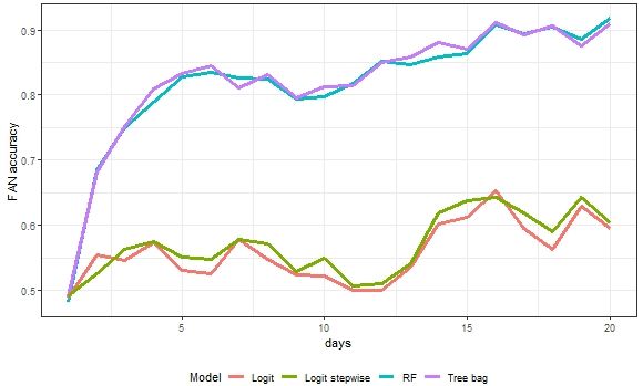
racy for logit and logit stepwise show that while there is some improvement in accuracy
                                    dicting stock
                                    between   1 andprice  direction
                                                     5 days  ahead, between   10 andaccuracy
                                                                     the prediction   20 days never
                                                                                               into the  future.
                                                                                                      gets aboveNotice   that The
                                                                                                                  0.6 (60%).   the pre-
                                                                                                                                    pre-
                                    diction accuracy   between   tree  bagging and  RF is very  similar.
                                    diction accuracy of the RFs and tree bagging methods show considerable improvement in
                                         The patterns
                                    accuracy   between of   prediction
                                                         1 and  10 days.accuracy for the
                                                                          Prediction     other for
                                                                                     accuracy   clean  energy ETFs
                                                                                                    predicting  stockare very
                                                                                                                       price     similar
                                                                                                                             direction
                                    to that which   was  described   for the PBW   clean energy   ETF   (Figures 5–8). For
                                    10 days into the future is over 85%. There is little variation in prediction accuracy
J. Risk Financial Manag. 2021, 14, 48
                                                                                                                            each
                                                                                                                            9 offor
                                                                                                                                    ETF,
                                                                                                                                 20 pre-
                                    the prediction
                                    dicting         accuracy
                                            stock price        of RFbetween
                                                          direction   and bagging  trees
                                                                              10 and  20 are
                                                                                         daysvery
                                                                                               intosimilar  and much
                                                                                                     the future. Noticemore
                                                                                                                         that accurate
                                                                                                                               the pre-
                                    than  that of the logit models.
                                    diction accuracy between tree bagging and RF is very similar.
                                 The patterns of prediction accuracy for the other clean energy ETFs are very similar
                            to that which was described for the PBW clean energy ETF (Figures 5–8). For each ETF,
                            the prediction accuracy of RF and bagging trees are very similar and much more accurate
                            than that of the logit models.

             Figure 4. This
                 Figure     figure
                        4. This     shows
                                figure     thethe
                                       shows    multi-period
                                                  multi-periodprediction  accuracyfor
                                                              prediction accuracy   for PBW
                                                                                      PBW    stock
                                                                                          stock    price
                                                                                                price     direction.
                                                                                                      direction.

                                      The patterns of prediction accuracy for the other clean energy ETFs are very similar to
                                that which was described for the PBW clean energy ETF (Figures 5–8). For each ETF, the
                                prediction accuracy of RF and bagging trees are very similar and much more accurate than
             Figure 4. This figure
                                thatshows
                                     of thethe multi-period
                                            logit models. prediction accuracy for PBW stock price direction.

            Figure 5. This figure shows the multi-period prediction accuracy for ICLN stock price direction.

            Figure 5. This
                Figure     figure
                       5. This     shows
                               figure     thethe
                                      shows    multi-period
                                                 multi-periodprediction  accuracyfor
                                                             prediction accuracy   for ICLN
                                                                                     ICLN    stock
                                                                                          stock    price
                                                                                                price     direction.
                                                                                                      direction.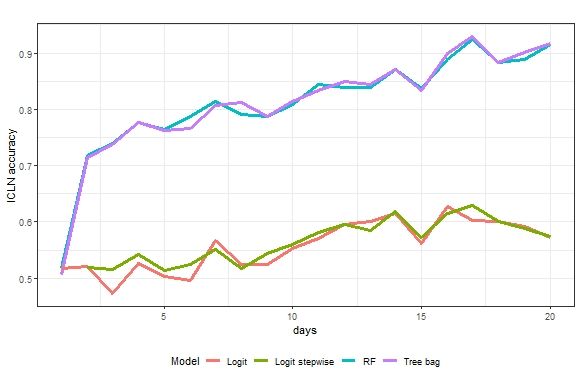
J. Risk Financial Manag. 2021, 14, x FOR PEER REVIEW                                                                   10 of 21

J. Risk Financial Manag. 2021, 14, x FOR PEER REVIEW                                                                   10 of 21
J. Risk Financial Manag. 2021, 14, 48                                                                                  10 of 20

                  Figure 6. This figure shows the multi-period prediction accuracy for QCLN stock price direction.

                  Figure 6. This figure shows the multi-period prediction accuracy for QCLN stock price direction.
                  Figure 6. This figure shows the multi-period prediction accuracy for QCLN stock price direction.

                    Figure 7. This figure shows the multi-period prediction accuracy for TAN stock price direction.
                   Figure 7. This figure shows the multi-period prediction accuracy for TAN stock price direction.
                                        Variable importance is used to determine which variables are most important in the
                   Figure 7. This figure shows the multi-period prediction accuracy for TAN stock price direction.
                                   RFs method. The mean decrease in accuracy (MD accuracy) is computed from the OOB
                                   data. The mean decrease in Gini (MD Gini) is a measure of node impurity. For each ETF at
                                   a 10-period forecast horizon, the OBV and MA200 are the two most important features in
                                   classifying clean stock price direction because they have the largest values of MD accuracy
                                   and MD Gini (Table 1). Further analysis for other forecasting horizons (not reported) shows
                                   that OBV and MA200 are also the two most important features in classifying clean stock
                                   price direction for other forecast horizons.
J. Risk Financial Manag. 2021, 14, 48 11 of 20
Table 1. Variable importance for predicting stock price direction.
PBW DOWN UP MD Accuracy MD Gini
RSI 27.25 25.08 39.08 83.52
STOFASTK 21.72 32.02 40.34 88.16
STOFASTD 23.57 30.88 41.60 87.75
STOSLOWD 24.69 37.53 48.96 92.61
ADX 47.96 35.96 59.22 113.76
MACD 31.61 32.30 49.15 95.34
MACD SIG 40.14 47.23 61.07 112.65
ROC 22.92 31.45 42.71 89.70
OBV 40.38 65.52 78.83 159.42
MA200 55.16 59.05 76.69 163.43
ICLN DOWN UP MD Accuracy MD Gini
RSI 25.22 26.11 43.73 84.61
STOFASTK 24.96 28.46 38.39 90.97
STOFASTD 24.25 29.09 40.42 90.17
STOSLOWD 27.16 33.68 45.18 99.41
ADX 42.63 45.21 57.23 118.19
MACD 31.44 33.40 52.24 98.33
MACD SIG 39.21 44.27 65.39 115.14
ROC 28.61 34.54 44.93 94.22
OBV 46.48 45.74 68.72 136.85
MA200 48.86 54.70 73.62 160.22
QCLN DOWN UP MD Accuracy MD Gini
RSI 21.12 27.75 38.94 80.18
STOFASTK 17.55 31.33 41.97 82.94
STOFASTD 19.79 25.81 38.73 79.04
STOSLOWD 22.80 28.07 39.61 84.70
ADX 48.87 39.29 57.54 121.13
MACD 26.27 36.55 49.99 100.96
MACD SIG 33.81 40.38 55.43 106.13
ROC 20.09 28.05 37.88 83.31
OBV 38.38 49.53 70.07 157.29
MA200 37.90 54.03 79.05 177.52
TAN DOWN UP MD Accuracy MD Gini
RSI 26.08 26.69 40.33 82.21
STOFASTK 24.88 30.74 40.60 89.81
STOFASTD 25.92 26.57 40.50 88.25
STOSLOWD 27.52 31.09 48.16 92.26
ADX 47.65 36.85 57.51 106.17
MACD 35.33 33.96 57.22 97.09
MACD SIG 46.82 41.11 63.02 119.30
ROC 26.14 35.20 44.29 86.07
OBV 40.31 44.17 62.35 143.25
MA200 57.22 65.98 87.26 188.03
FAN DOWN UP MD Accuracy MD Gini
RSI 19.60 31.69 40.69 83.58
STOFASTK 29.17 28.86 40.30 89.74
STOFASTD 24.42 31.22 39.79 85.90
STOSLOWD 19.88 34.82 43.65 87.54
ADX 43.40 43.42 61.05 106.36
MACD 30.11 35.62 53.46 95.40
MACD SIG 38.86 44.22 63.47 107.28
ROC 29.82 32.87 42.90 88.70
OBV 53.00 57.56 68.49 166.36
MA200 48.83 65.65 83.29 169.59
This table shows the RFs variable importance of the technical analysis indicators measured using mean decrease in
accuracy (MD accuracy) and mean decrease in GINI (MD Gini). Values reported for a 10-period forecast horizon.J. Risk Financial Manag. 2021, 14, x FOR PEER REVIEW 11 of 21
J. Risk Financial Manag. 2021, 14, 48 12 of 20
Figure 8. This figure shows the multi-period prediction accuracy for FAN stock price direction.
Figure 8. This figure shows the multi-period prediction accuracy for FAN stock price direction.
Figures 4–8 show the overall prediction accuracy. Another interesting question to ask
Variable importance is used to determine which variables are most important in the
is how the prediction accuracy compares between positive prediction values and negative
RFs method. The mean decrease in accuracy (MD accuracy) is computed from the OOB
prediction values.
data. The mean Positive
decrease in predictive
Gini (MD Gini)value is is the proportion
a measure of node of predicted
impurity. Forpositive
each ETFcases
that are actually positive. An alternative way to think about this is,
at a 10-period forecast horizon, the OBV and MA200 are the two most important features when a model predicts
a in
positive case, how often is it correct?
classifying clean stock price direction because they have the largest values of MD accu-
racy
J. Risk Financial Manag. 2021, 14, x FOR Figure
PEERand MD9 reports
REVIEW the positive
Gini (Table 1). Further prediction
analysis forvalue forforecasting
other PBW. Thishorizons
plot shows
(not how 13accurate
reported)
of 21
the models are in prediction the positive price direction. The RFs and
shows that OBV and MA200 are also the two most important features in classifying clean tree bagging methods
are more
stock accurate
price directionthan
forthe logit
other methods.
forecast After 5 days, the RFs and tree bagging methods
horizons.
have an accuracy
reaches higher thanof over
70%.80%
The while
patternthe
of accuracy of the logit
positive predictive methods
value for thenever
otherreaches higher
ETFs (Fig-
Table
than 1. Variable importancepositive
for predicting stock price direction.
ures70%. The
10–13) arepattern
similar of predictive
to what is observed for value
PBW. Forfor the
eachother
ETF, ETFs (Figures
after 10 days the10–13)
posi- are
similar to what values
tive predictive
PBW is observed
for RFsfor
DOWN andPBW. For
bagging each
UP are ETF,0.80
above after
MD 10indays
and mostthe
Accuracy positive
cases above
MD predictive
0.85.
Gini
values forRSI
RFs and bagging
27.25
are above 0.80
25.08
and in most cases
39.08
above 0.85. 83.52
STOFASTK 21.72 32.02 40.34 88.16
STOFASTD 23.57 30.88 41.60 87.75
STOSLOWD 24.69 37.53 48.96 92.61
ADX 47.96 35.96 59.22 113.76
MACD 31.61 32.30 49.15 95.34
MACD SIG 40.14 47.23 61.07 112.65
ROC 22.92 31.45 42.71 89.70
OBV 40.38 65.52 78.83 159.42
MA200 55.16 59.05 76.69 163.43
ICLN DOWN UP MD Accuracy MD Gini
RSI 25.22 26.11 43.73 84.61
STOFASTK 24.96 28.46 38.39 90.97
STOFASTD 24.25 29.09 40.42 90.17
STOSLOWD 27.16 33.68 45.18 99.41
ADX 42.63 45.21 57.23 118.19
MACD 31.44 33.40 52.24 98.33
Figure 9. This figure shows the multi-period positive predictive values accuracy for PBW stock price direction.
Figure 9. This figure shows the multi-period positive predictive values accuracy for PBW stock price direction.J. Risk Financial Manag. 2021, 14, 48 13 of 20
Figure 9. This figure shows the multi-period positive predictive values accuracy for PBW stock price direction.
J. Risk Financial Manag. 2021, 14, x FOR PEER REVIEW 14 of 21
Figure 10. This figure shows the multi-period positive predictive values accuracy for ICLN stock price direction.
Figure 10. This figure shows the multi-period positive predictive values accuracy for ICLN stock price direction.
Figure 11. This figure shows the multi-period positive predictive values accuracy for QCLN stock price direction.
Figure 11. This figure shows the multi-period positive predictive values accuracy for QCLN stock price direction.J. Risk Financial Manag. 2021, 14, 48 14 of 20
Figure 11. This figure shows the multi-period positive predictive values accuracy for QCLN stock price direction.
J. Risk Financial Manag. 2021, 14, x FOR PEER REVIEW 15 of 21
Figure 12. This figure shows the multi-period positive predictive values accuracy for TAN stock price direction.
Figure 12. This figure shows the multi-period positive predictive values accuracy for TAN stock price direction.
Figure
Figure 13.
13. This
This figure
figure shows
shows the
the multi-period
multi-period positive predictive values
positive predictive values accuracy
accuracy for
for FAN
FAN stock
stock price
price direction.
direction.
Figures 14–18 show the negative predictive value. The negative predictive value is
the proportion of predicted negative cases relative to the actual number of of negative
negative cases.
cases.
Figure 14 reports the negative predictive value for PBW. This plot plot shows
shows how
how accurate
accurate
the models are in predicting the down
down stock
stock price
price direction.
direction. The RFs and tree bagging
bagging
methods
methods are more accurate than the logit models. For
For the RFs and tree bagging models,
accuracy increases from 0.5 to 0.8 between 1 and 5 days. After 10 days negative predictive
value fluctuates between 0.85 and 0.90. The pattern of negative predictive value for the
ETFs (Figures
other ETFs (Figures15–18)
15–18)are
aresimilar
similartotowhat
whatisis observed
observed forfor PBW.
PBW. ForFor each
each ETF,
ETF, after
after 10
days the negative predictive values for RFs and bagging are above 0.80 and in most cases
above 0.85.the proportion of predicted negative cases relative to the actual number of negative cases.
Figure 14 reports the negative predictive value for PBW. This plot shows how accurate
the models are in predicting the down stock price direction. The RFs and tree bagging
methods are more accurate than the logit models. For the RFs and tree bagging models,
J. Risk Financial Manag. 2021, 14, 48 15 of 20
accuracy increases from 0.5 to 0.8 between 1 and 5 days. After 10 days negative predictive
value fluctuates between 0.85 and 0.90. The pattern of negative predictive value for the
other ETFs (Figures 15–18) are similar to what is observed for PBW. For each ETF, after 10
days the the
10 days negative predictive
negative values
predictive for RFs
values for and
RFs bagging are above
and bagging 0.80 and
are above 0.80inand
most
in cases
most
above 0.85.
cases above 0.85.
J. Risk Financial Manag. 2021, 14, x FOR PEER REVIEW 16 of 21
Figure
Figure 14.
14. This
This figure
figure shows
shows the
the multi-period
multi-period negative
negative predictive values accuracy for PBW stock price direction.
Figure 15. This figure shows the multi-period negative predictive values accuracy for ICLN stock price direction.
Figure 15. This figure shows the multi-period negative predictive values accuracy for ICLN stock price direction.J. Risk Financial Manag. 2021, 14, 48 16 of 20
Figure 15. This figure shows the multi-period negative predictive values accuracy for ICLN stock price direction.
J. Risk Financial Manag. 2021, 14, x FOR PEER REVIEW 17 of 21
Figure 16. This figure shows the multi-period negative predictive values accuracy for QCLN stock price direction.
Figure 16. This figure shows the multi-period negative predictive values accuracy for QCLN stock price direction.
Figure 17. This figure shows the multi-period negative predictive values accuracy for TAN stock price direction.
Figure 17. This figure shows the multi-period negative predictive values accuracy for TAN stock price direction.J. Risk Financial Manag. 2021, 14, 48 17 of 20
Figure 17. This figure shows the multi-period negative predictive values accuracy for TAN stock price direction.
Figure 18. This figure shows the multi-period negative predictive values accuracy for FAN stock price direction.
Figure 18. This figure shows the multi-period negative predictive values accuracy for FAN stock price direction.
To summarize, the main take-away from this research is that RFs and tree bagging
provideTo summarize,
much betterthe main take-away
predicting accuracy from
thenthis research
logit is that RFs
or step-wise logit.and tree
The bagging
prediction
provide much better predicting accuracy then logit or step-wise logit. The
accuracy between bagging and RFs is very similar indicating that either method is very prediction ac-
curacy between
useful for bagging
predicting and RFs
the stock is direction
price very similar indicating
of clean energythat either
ETFs. Themethod is very
prediction use-
accuracy
ful
for for
RF predicting the stock
and tree bagging priceisdirection
models over 80% offor
clean energy
forecast ETFs. The
horizons of 10prediction accuracy
days or more. The
for RF and tree bagging models is over 80% for forecast horizons of 10 days or
positive predictive values and negative predictive values are similar indicating that there ismore. The
little asymmetry between the up and down prediction classifications.
4. Discussion
The research in this paper shows that RFs produce more accurate clean energy stock
price direction forecasts than logit models. These results add to a growing body of research
that shows machine learning methods like RFs have considerable stock price direction
predictive performance (Ballings et al. 2015; Basak et al. 2019; Lohrmann and Luukka 2019;
Weng et al. 2018; Ampomah et al. 2020). None of these studies, however, consider clean
energy stock prices. This paper appears to be the first paper to use ML methods to predict
clean energy stock price direction.
There is literature on clean energy equity dynamics that largely focuses on the impact
of oil prices on clean energy stock returns (Bondia et al. 2016; Dutta 2017; Dutta et al. 2018;
Elie et al. 2019; Gupta 2017; Henriques and Sadorsky 2008; Kumar et al. 2012; Maghyereh
et al. 2019; Managi and Okimoto 2013; Reboredo 2015; Reboredo et al. 2017b; Reboredo and
Ugolini 2018; Uddin et al. 2019; Wen et al. 2014). Popular modelling approaches include
multifactor models (Henriques and Sadorsky 2008; Gupta 2017; Reboredo et al. 2017b; Bohl
et al. 2013; Sadorsky 2012), vector autoregressions (Kumar et al. 2012; Dutta et al. 2018),
or other approaches like wavelets (Maghyereh et al. 2019; Reboredo et al. 2017a), copulas
(Reboredo 2015), and quantiles (Uddin et al. 2019; Dawar et al. 2021). While this research is
important in establishing that oil prices have a significant impact on clean energy stock
prices the focus has not been on forecasting clean energy stock prices.
The results of this present paper could be combined with some of the knowledge
discussed in the previous paragraph to expand the feature set used in estimating RFs. It may,
for example, be useful to include other variables like oil prices in the set of features used in
the estimation of RFs. A comparison could be made between feature sets that are basedJ. Risk Financial Manag. 2021, 14, 48 18 of 20
on technical indicators and feature sets that include oil prices and other macroeconomic
variables to see if macroeconomic variables offer additional insight into predicting clean
energy stock price direction.
5. Conclusions
There is a growing interest in investing in clean energy companies and some of the
major drivers behind this interest include climate change, green consumers, energy security,
fossil fuel divestment, and technological innovation. Investors in clean energy equities
would benefit from a better understanding of how to predict clean energy stock prices.
There is, however, a noticeable lack of information on this topic. This is the gap in the
literature that this paper fills.
Building on the existing finance literature that shows stock price direction is easier
to predict than stock prices and recent developments in machine learning showing that
ML techniques offer an improvement in prediction over conventional regression-based
approaches, this paper uses RFs and decision tree bagging to predict clean energy equity
stock price direction. RFs and decision tree bagging are easier to explain and estimate
than other ML techniques like ANNs or SVMs, but RFs appear to be underutilized in the
existing literature. Five well known and actively traded clean energy ETFs are chosen for
study. For each ETF, prediction accuracy is assessed using a time horizon of one day to
twenty days (which is approximately one month of trading days).
RFs and tree bagging show much better stock price prediction accuracy then logit or
step-wise logit. The prediction accuracy from bagging and RFs is very similar indicating
that either method is very useful for predicting the stock price direction of clean energy
ETFs. The prediction accuracy for RF and tree bagging models is over 80% for forecast
horizons of 10 days or more. For a 20-day forecast horizon, tree bagging and random
forests methods produce accuracy rates of between 85% and 90% while logit models
produce accuracy rates of between 55% and 60%. These results are in agreement with other
research that shows RFs to have a high stock price predictive accuracy (Ballings et al. 2015;
Basak et al. 2019; Lohrmann and Luukka 2019; Weng et al. 2018; Ampomah et al. 2020).
The positive predictive values and negative predictive values indicate that there is little
asymmetry between the up and down prediction classifications.
There are several different avenues for future research. First, this paper has focused
on the comparison between bagging decision trees, RFs, and logit models. A deeper
analysis could include other ML methods like boosting, ANN and SVM. Second, this paper
used a set of well-known technical indicators for features. The feature space could be
expanded to include additional technical indicators or other variables like oil prices or
other macroeconomic variables. Third, the analysis in this paper was conducted using
ETFs. It may also be of interest to apply machine learning techniques to company specific
clean energy stock price prediction.
Funding: This research received no external funding.
Institutional Review Board Statement: Not applicable.
Informed Consent Statement: Not applicable.
Data Availability Statement: The data used in this study are available from Yahoo Finance at
https://finance.yahoo.com/.
Acknowledgments: I thank the Schulich School of Business for internal financial support. I thank
the reviewers for helpful comments.
Conflicts of Interest: The author declares no conflict of interest.J. Risk Financial Manag. 2021, 14, 48 19 of 20
References
Ampomah, Ernest Kwame, Zhiguang Qin, and Gabriel Nyame. 2020. Evaluation of Tree-Based Ensemble Machine Learning Models in
Predicting Stock Price Direction of Movement. Information 11: 332. [CrossRef]
Andreoni, Valeria. 2020. The Energy Metabolism of Countries: Energy Efficiency and Use in the Period That Followed the Global
Financial Crisis. Energy Policy 139: 111304. [CrossRef]
Atsalakis, George S., and Kimon P. Valavanis. 2009. Surveying Stock Market Forecasting Techniques—Part II: Soft Computing Methods.
Expert Systems with Applications 36, Pt 2: 5932–41. [CrossRef]
Ballings, Michel, Dirk Van den Poel, Nathalie Hespeels, and Ruben Gryp. 2015. Evaluating Multiple Classifiers for Stock Price Direction
Prediction. Expert Systems with Applications 42: 7046–56. [CrossRef]
Basak, Suryoday, Saibal Kar, Snehanshu Saha, Luckyson Khaidem, and Sudeepa Roy Dey. 2019. Predicting the Direction of Stock
Market Prices Using Tree-Based Classifiers. The North American Journal of Economics and Finance 47: 552–67. [CrossRef]
Bohl, Martin T., Philipp Kaufmann, and Patrick M. Stephan. 2013. From Hero to Zero: Evidence of Performance Reversal and
Speculative Bubbles in German Renewable Energy Stocks. Energy Economics 37: 40–51. [CrossRef]
Bondia, Ripsy, Sajal Ghosh, and Kakali Kanjilal. 2016. International Crude Oil Prices and the Stock Prices of Clean Energy and
Technology Companies: Evidence from Non-Linear Cointegration Tests with Unknown Structural Breaks. Energy 101: 558–65.
[CrossRef]
Breiman, Leo. 2001. Random Forests. Machine Learning 45: 5–32. [CrossRef]
Breiman, Leo, Adele Cutler, Andy Liaw, and Matthew Wiener. 2018. RandomForest: Breiman and Cutler’s Random Forests
for Classification and Regression. R Package Version 4.6-14. Available online: https://www.stat.berkeley.edu/~breiman/
RandomForests/ (accessed on 25 August 2020).
Bustos, O, and A. Pomares-Quimbaya. 2020. Stock Market Movement Forecast: A Systematic Review. Expert Systems with Applications
156: 113464. [CrossRef]
Christoffersen, Peter F., and Francis X. Diebold. 2006. Financial Asset Returns, Direction-of-Change Forecasting, and Volatility
Dynamics. Management Science 52: 1273–87. [CrossRef]
Dawar, Ishaan, Anupam Dutta, Elie Bouri, and Tareq Saeed. 2021. Crude Oil Prices and Clean Energy Stock Indices: Lagged and
Asymmetric Effects with Quantile Regression. Renewable Energy 163: 288–99. [CrossRef]
Dutta, Anupam. 2017. Oil Price Uncertainty and Clean Energy Stock Returns: New Evidence from Crude Oil Volatility Index. Journal of
Cleaner Production 164: 1157–66. [CrossRef]
Dutta, Anupam, Elie Bouri, and Md Hasib Noor. 2018. Return and Volatility Linkages between CO2 Emission and Clean Energy Stock
Prices. Energy 164: 803–10. [CrossRef]
Elie, Bouri, Jalkh Naji, Anupam Dutta, and Gazi Salah Uddin. 2019. Gold and Crude Oil as Safe-Haven Assets for Clean Energy Stock
Indices: Blended Copulas Approach. Energy 178: 544–53. [CrossRef]
Frankfurt School-UNEP Centre/BNEF. 2020. Global Trends in Renewable Energy Investment 2020. Frankfurt am Main: Frankfurt School of
Finance & Management gGmbH.
Ghoddusi, Hamed, Germán G. Creamer, and Nima Rafizadeh. 2019. Machine Learning in Energy Economics and Finance: A Review.
Energy Economics 81: 709–27. [CrossRef]
Gray, Wesley, and Jack Vogel. 2016. Quantitative Momentum: A Practitioner’s Guide to Building a Momentum-Based Stock Selection System.
Hoboken: John Wiley & Sons.
Gupta, Kartick. 2017. Do Economic and Societal Factors Influence the Financial Performance of Alternative Energy Firms? Energy
Economics 65: 172–82. [CrossRef]
Henrique, Bruno Miranda, Vinicius Amorim Sobreiro, and Herbert Kimura. 2019. Literature Review: Machine Learning Techniques
Applied to Financial Market Prediction. Expert Systems with Applications 124: 226–51. [CrossRef]
Henriques, Irene, and Perry Sadorsky. 2008. Oil Prices and the Stock Prices of Alternative Energy Companies. Energy Economics 30:
998–1010. [CrossRef]
James, Gareth, Daniela Witten, Trevor Hastie, and Robert Tibshirani. 2013. An Introduction to Statistical Learning: With Applications in R.
Springer Texts in Statistics. New York: Springer. [CrossRef]
Khan, Wasiat, Mustansar Ali Ghazanfar, Muhammad Awais Azam, Amin Karami, Khaled H. Alyoubi, and Ahmed S. Alfakeeh.
2020. Stock Market Prediction Using Machine Learning Classifiers and Social Media, News. Journal of Ambient Intelligence and
Humanized Computing. [CrossRef]
Kumar, Surender, Shunsuke Managi, and Akimi Matsuda. 2012. Stock Prices of Clean Energy Firms, Oil and Carbon Markets: A Vector
Autoregressive Analysis. Energy Economics 34: 215–26. [CrossRef]
Leung, Mark T., Hazem Daouk, and An-Sing Chen. 2000. Forecasting Stock Indices: A Comparison of Classification and Level
Estimation Models. International Journal of Forecasting 16: 173–90. [CrossRef]
Lo, Andrew W., Harry Mamaysky, and Jiang Wang. 2000. Foundations of Technical Analysis: Computational Algorithms, Statistical
Inference, and Empirical Implementation. The Journal of Finance 55: 1705–65. [CrossRef]
Lohrmann, Christoph, and Pasi Luukka. 2019. Classification of Intraday S&P500 Returns with a Random Forest. International Journal of
Forecasting 35: 390–407. [CrossRef]
Maghyereh, Aktham I., Basel Awartani, and Hussein Abdoh. 2019. The Co-Movement between Oil and Clean Energy Stocks:
A Wavelet-Based Analysis of Horizon Associations. Energy 169: 895–913. [CrossRef]You can also read