A Survey of Safety and Trustworthiness of Deep Neural Networks: Verification, Testing, Adversarial Attack and Defence, and Interpretability - TU ...
←
→
Page content transcription
If your browser does not render page correctly, please read the page content below
A Survey of Safety and Trustworthiness of Deep
                                              Neural Networks: Verification, Testing,
arXiv:1812.08342v5 [cs.LG] 31 May 2020

                                               Adversarial Attack and Defence, and
                                                         Interpretability ∗
                                          Xiaowei Huang1 , Daniel Kroening2 , Wenjie Ruan3 , James Sharp4 ,
                                            Youcheng Sun5 , Emese Thamo1 , Min Wu2 , and Xinping Yi1
                                                                   1
                                                             University of Liverpool, UK,
                                              {xiaowei.huang, emese.thamo, xinping.yi}@liverpool.ac.uk
                                         2
                                           University of Oxford, UK, {daniel.kroening, min.wu}@cs.ox.ac.uk
                                               3
                                                 Lancaster University, UK, wenjie.ruan@lancaster.ac.uk
                                              4
                                                Defence Science and Technology Laboratory (Dstl), UK,
                                                                 jsharp1@dstl.gov.uk
                                             5
                                               Queen’s University Belfast, UK, youcheng.sun@qub.ac.uk

                                             In the past few years, significant progress has been made on deep neural
                                         networks (DNNs) in achieving human-level performance on several long-standing
                                         tasks. With the broader deployment of DNNs on various applications, the con-
                                         cerns over their safety and trustworthiness have been raised in public, especially
                                         after the widely reported fatal incidents involving self-driving cars. Research to
                                         address these concerns is particularly active, with a significant number of papers
                                         released in the past few years. This survey paper conducts a review of the current
                                         research effort into making DNNs safe and trustworthy, by focusing on four
                                         aspects: verification, testing, adversarial attack and defence, and interpretability.
                                         In total, we survey 202 papers, most of which were published after 2017.

                                         Contents
                                         1 Introduction                                                                              6
                                           1.1 Certification . . . . . . . . . . . . . . . . . . . . . . . . . . . . . .             7
                                            ∗ This work is supported by the UK EPSRC projects on Offshore Robotics for Certification of

                                         Assets (ORCA) [EP/R026173/1] and End-to-End Conceptual Guarding of Neural Architectures
                                         [EP/T026995/1], and ORCA Partnership Resource Fund (PRF) on Towards the Accountable
                                         and Explainable Learning-enabled Autonomous Robotic Systems, as well as the UK Dstl
                                         projects on Test Coverage Metrics for Artificial Intelligence.

                                                                                       0
1.2   Explanation . . . . . . . . . . . . . . . . . . . . . . . . . . . . . .                                 8
   1.3   Organisation of This Survey . . . . . . . . . . . . . . . . . . . . .                                   8

2 Preliminaries                                                                                                 10
  2.1 Deep Neural Networks . . . . . . . . .        .   .   .   .   .   .   .   .   .   .   .   .   .   .   .   10
  2.2 Verification . . . . . . . . . . . . . . .    .   .   .   .   .   .   .   .   .   .   .   .   .   .   .   12
  2.3 Testing . . . . . . . . . . . . . . . . .     .   .   .   .   .   .   .   .   .   .   .   .   .   .   .   12
  2.4 Interpretability . . . . . . . . . . . . .    .   .   .   .   .   .   .   .   .   .   .   .   .   .   .   13
  2.5 Distance Metric and d-Neighbourhood           .   .   .   .   .   .   .   .   .   .   .   .   .   .   .   14

3 Safety Problems and Safety Properties                                                                         15
  3.1 Adversarial Examples . . . . . . . . . .          .   .   .   .   .   .   .   .   .   .   .   .   .   .   16
  3.2 Local Robustness Property . . . . . . .           .   .   .   .   .   .   .   .   .   .   .   .   .   .   17
  3.3 Output Reachability Property . . . . . .          .   .   .   .   .   .   .   .   .   .   .   .   .   .   18
  3.4 Interval Property . . . . . . . . . . . . .       .   .   .   .   .   .   .   .   .   .   .   .   .   .   19
  3.5 Lipschitzian Property . . . . . . . . . .         .   .   .   .   .   .   .   .   .   .   .   .   .   .   19
  3.6 Relationship between Properties . . . .           .   .   .   .   .   .   .   .   .   .   .   .   .   .   20
  3.7 Instancewise Interpretability . . . . . . .       .   .   .   .   .   .   .   .   .   .   .   .   .   .   21

4 Verification                                                                                                  22
  4.1 Approaches with Deterministic Guarantees . . . . . . .                                . . . . .           23
       4.1.1 SMT/SAT . . . . . . . . . . . . . . . . . . . . . .                            . . . . .           23
       4.1.2 Mixed Integer Linear Programming (MILP) . . .                                  . . . . .           24
  4.2 Approaches to Compute an Approximate Bound . . . .                                    . . . . .           25
       4.2.1 Abstract Interpretation . . . . . . . . . . . . . .                            . . . . .           26
       4.2.2 Convex Optimisation based Methods . . . . . . .                                . . . . .           27
       4.2.3 Interval Analysis . . . . . . . . . . . . . . . . . .                          . . . . .           27
       4.2.4 Output Reachable Set Estimation . . . . . . . .                                . . . . .           28
       4.2.5 Linear Approximation of ReLU Networks . . . .                                  . . . . .           28
  4.3 Approaches to Compute Converging Bounds . . . . . . .                                 . . . . .           28
       4.3.1 Layer-by-Layer Refinement . . . . . . . . . . . .                              . . . . .           29
       4.3.2 Reduction to A Two-Player Turn-based Game .                                    . . . . .           29
       4.3.3 Global Optimisation Based Approaches . . . . .                                 . . . . .           30
  4.4 Approaches with Statistical Guarantees . . . . . . . . .                              . . . . .           30
       4.4.1 Lipschitz Constant Estimation by Extreme Value                                 Theory              30
       4.4.2 Robustness Estimation . . . . . . . . . . . . . . .                            . . . . .           30
  4.5 Computational Complexity of Verification . . . . . . . .                              . . . . .           31
  4.6 Summary . . . . . . . . . . . . . . . . . . . . . . . . . .                           . . . . .           31

5 Testing                                                                                                       33
  5.1 Coverage Criteria for DNNs . . . . . . . . . .                . . . . . .             .   .   .   .   .   33
       5.1.1 Neuron Coverage . . . . . . . . . . . .                . . . . . .             .   .   .   .   .   34
       5.1.2 Safety Coverage . . . . . . . . . . . .                . . . . . .             .   .   .   .   .   35
       5.1.3 Extensions of Neuron Coverage . . . .                  . . . . . .             .   .   .   .   .   35
       5.1.4 Modified Condition/Decision Coverage                   (MC/DC)                 .   .   .   .   .   36
       5.1.5 Quantitative Projection Coverage . . .                 . . . . . .             .   .   .   .   .   39

                                         1
5.1.6 Surprise Coverage . . . . . . . . . . . . . . . . . . . . . . 39
5.1.7 Comparison between Existing Coverage Criteria . . . . . 39
5.2 Test Case Generation . . . . . . . . . . . . . . . . . . . . . . . . 40
5.2.1 Input Mutation . . . . . . . . . . . . . . . . . . . . . . . . 40
5.2.2 Fuzzing . . . . . . . . . . . . . . . . . . . . . . . . . . . . 40
5.2.3 Symbolic Execution and Testing . . . . . . . . . . . . . . 41
5.2.4 Testing using Generative Adversarial Networks . . . . . . 42
5.2.5 Differential Analysis . . . . . . . . . . . . . . . . . . . . . 42
5.3 Model-Level Mutation Testing . . . . . . . . . . . . . . . . . . . . 42
5.4 Summary . . . . . . . . . . . . . . . . . . . . . . . . . . . . . . . 43
6 Adversarial Attack and Defence 45
6.1 Adversarial Attacks . . . . . . . . . . . . . . . . . . . . . . . . . 45
6.1.1 Limited-Memory BFGS Algorithm (L-BFGS) . . . . . . . 46
6.1.2 Fast Gradient Sign Method (FGSM) . . . . . . . . . . . . 46
6.1.3 Jacobian Saliency Map based Attack (JSMA) . . . . . . . 47
6.1.4 DeepFool: A Simple and Accurate Method to Fool Deep
Neural Networks . . . . . . . . . . . . . . . . . . . . . . . 47
6.1.5 Carlini & Wagner Attack . . . . . . . . . . . . . . . . . . 48
6.2 Adversarial Attacks by Natural Transformations . . . . . . . . . 48
6.2.1 Rotation and Translation . . . . . . . . . . . . . . . . . . 49
6.2.2 Spatially Transformed Adversarial Examples . . . . . . . 49
6.2.3 Towards Practical Verification of Machine Learning: The
Case of Computer Vision Systems (VeriVis) . . . . . . . . 49
6.3 Input-Agnostic Adversarial Attacks . . . . . . . . . . . . . . . . . 50
6.3.1 Universal Adversarial Perturbations . . . . . . . . . . . . 50
6.3.2 Generative Adversarial Perturbations . . . . . . . . . . . 51
6.4 Other Types of Universal Adversarial Perturbations . . . . . . . 51
6.5 Summary of Adversarial Attack Techniques . . . . . . . . . . . . 52
6.6 Adversarial Defence . . . . . . . . . . . . . . . . . . . . . . . . . 52
6.6.1 Adversarial Training . . . . . . . . . . . . . . . . . . . . . 52
6.6.2 Defensive Distillation . . . . . . . . . . . . . . . . . . . . 54
6.6.3 Dimensionality Reduction . . . . . . . . . . . . . . . . . . 54
6.6.4 Input Transformations . . . . . . . . . . . . . . . . . . . . 54
6.6.5 Combining Input Discretisation with Adversarial Training 55
6.6.6 Activation Transformations . . . . . . . . . . . . . . . . . 55
6.6.7 Characterisation of Adversarial Region . . . . . . . . . . . 56
6.6.8 Defence against Data Poisoning Attack . . . . . . . . . . 56
6.7 Certified Adversarial Defence . . . . . . . . . . . . . . . . . . . . 56
6.7.1 Robustness through Regularisation in Training . . . . . . 56
6.7.2 Robustness through Training Objective . . . . . . . . . . 57
6.8 Summary of Adversarial Defence Techniques . . . . . . . . . . . 57
27 Interpretability 59
7.1 Instance-wise Explanation by Visualising a Synthesised Input . . 59
7.1.1 Optimising Over a Hidden Neuron . . . . . . . . . . . . . 59
7.1.2 Inverting Representation . . . . . . . . . . . . . . . . . . . 59
7.2 Instancewise Explanation by Ranking . . . . . . . . . . . . . . . 60
7.2.1 Local Interpretable Model-agnostic Explanations (LIME) 60
7.2.2 Integrated Gradients . . . . . . . . . . . . . . . . . . . . . 61
7.2.3 Layer-wise Relevance Propagation (LRP) . . . . . . . . . 61
7.2.4 Deep Learning Important FeaTures (DeepLIFT) . . . . . 62
7.2.5 Gradient-weighted Class Activation Mapping (GradCAM) 62
7.2.6 SHapley Additive exPlanation (SHAP) . . . . . . . . . . . 62
7.2.7 Prediction Difference Analysis . . . . . . . . . . . . . . . . 63
7.2.8 Testing with Concept Activation Vector (TCAV) . . . . . 63
7.2.9 Learning to Explain (L2X) . . . . . . . . . . . . . . . . . 64
7.3 Instancewise Explanation by Saliency Maps . . . . . . . . . . . . 64
7.3.1 Gradient-based Methods . . . . . . . . . . . . . . . . . . . 64
7.3.2 Perturbation-based Methods . . . . . . . . . . . . . . . . 65
7.4 Model Explanation by Influence Functions . . . . . . . . . . . . . 65
7.5 Model Explanation by Simpler Models . . . . . . . . . . . . . . . 66
7.5.1 Rule Extraction . . . . . . . . . . . . . . . . . . . . . . . 66
7.5.2 Decision Tree Extraction . . . . . . . . . . . . . . . . . . 66
7.5.3 Linear Classifiers to Approximate Piece-wise Linear Neural
Networks . . . . . . . . . . . . . . . . . . . . . . . . . . . 67
7.5.4 Automata Extraction from Recurrent Neural Networks . . 67
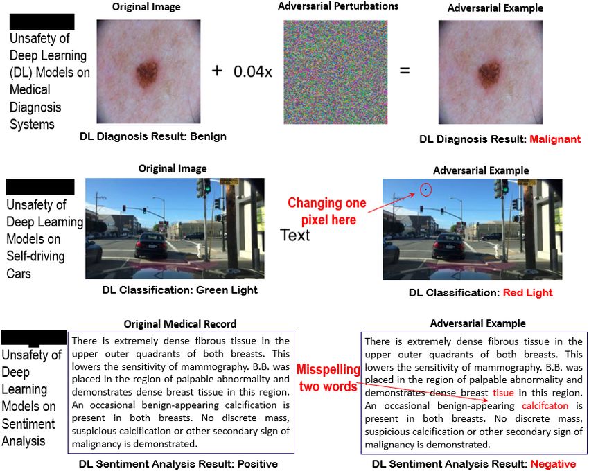
7.6 Information-flow Explanation by Information Theoretical Methods 67
7.6.1 Information Bottleneck Method . . . . . . . . . . . . . . . 67
7.6.2 Information Plane . . . . . . . . . . . . . . . . . . . . . . 68
7.6.3 From Deterministic to Stochastic DNNs . . . . . . . . . . 69
7.7 Summary . . . . . . . . . . . . . . . . . . . . . . . . . . . . . . . 70
8 Future Challenges 71
8.1 Distance Metrics closer to Human Perception . . . . . . . . . . . 71
8.2 Improvement to Robustness . . . . . . . . . . . . . . . . . . . . . 71
8.3 Other Machine Learning Models . . . . . . . . . . . . . . . . . . 72
8.4 Verification Completeness . . . . . . . . . . . . . . . . . . . . . . 72
8.5 Scalable Verification with Tighter Bounds . . . . . . . . . . . . . 73
8.6 Validation of Testing Approaches . . . . . . . . . . . . . . . . . . 73
8.7 Learning-Enabled Systems . . . . . . . . . . . . . . . . . . . . . . 74
8.8 Distributional Shift, Out-of-Distribution Detection, and Run-time
Monitoring . . . . . . . . . . . . . . . . . . . . . . . . . . . . . . 74
8.9 Unifying Formulation of Interpretability . . . . . . . . . . . . . . 75
8.10 Application of Interpretability to other Tasks . . . . . . . . . . . 75
8.11 Human-in-the-Loop . . . . . . . . . . . . . . . . . . . . . . . . . . 76
9 Conclusions 76
3Symbols and Acronyms
List of Symbols
We provide an incomplete list of symbols that will be used in the survey.
N a neural network
f function represented by a neural network
W weight
b bias
nk,l l-th neuron on the k-th layer
vk,l activation value of the l-th neuron on the k-th layer
` loss function
x input
y output
η a region around a point
∆ a set of manipulations
R a set of test conditions
T test suite
G regularisation term
X the ground truth distribution of the inputs
error tolerance bound
L0 (-norm) L0 norm distance metric
L1 (-norm) L1 norm distance metric
L2 (-norm) L2 norm distance metric
L∞ (-norm) L infinity norm distance metric
E probabilistic expectation
4List of Acronyms
DNN Deep Neural Network
AI Artificial Intelligence
DL Deep Learning
MILP Mixed Integer Linear Programming
SMT Satisfiability Modulo Theory
MC/DC Modified Condition/Decision Coverage
B&B Branch and Bound
ReLU Rectified Linear Unit
51 Introduction
In the past few years, significant progress has been made in the development
of deep neural networks (DNNs), which now outperform humans in several
difficult tasks, such as image classification [Russakovsky et al., 2015], natural
language processing [Collobert et al., 2011], and two-player games [Silver et al.,
2017]. Given the prospect of a broad deployment of DNNs in a wide range of
applications, concerns regarding the safety and trustworthiness of this approach
have been raised [Tes, 2018, Ube, 2018]. There is significant research that aims
to address these concerns, with many publications appearing in the past few
years.
Whilst it is difficult to cover all related research activities, we strive to survey
the past and current research efforts on making the application of DNNs safe
and trustworthy. Figure 1 visualises the rapid growth of this area: it gives the
number of surveyed papers per calendar year, starting from 2008 to 2018. In
total, we surveyed 202 papers.
Trust, or trustworthiness, is a general term and its definition varies in
different contexts. Our definition is based on the practice that has been widely
adopted in established industries, e.g., automotive and avionics. Specifically,
trustworthiness is addressed predominantly within two processes: a certification
process and an explanation process. The certification process is held before
the deployment of the product to make sure that it functions correctly (and
safely). During the certification process, the manufacturer needs to demonstrate
to the relevant certification authority, e.g., the European Aviation Safety Agency
or the Vehicle Certification Agency, that the product behaves correctly with
respect to a set of high-level requirements. The explanation process is held
whenever needed during the lifetime of the product. The user manual explains a
set of expected behaviours of the product that its user may frequently experience.
More importantly, an investigation can be conducted, with a formal report
produced, to understand any unexpected behaviour of the product. We believe
that a similar practice should be carried out when working with data-driven
deep learning systems. That is, in this survey, we address trustworthiness based
on the following concept:
Trustworthiness = Certification + Explanation
In other words, a user is able to trust a system if the system has been certified by
a certification authority and any of its behaviour can be well explained. Moreover,
we will discuss briefly in Section 8.11 our view on the impact of human-machine
interactions on trust.
In this survey, we will consider the advancement of enabling techniques for
both the certification and the explanation processes of DNNs. Both processes
are challenging, owing to the black-box nature of DNNs and the lack of rigorous
foundations.
6Figure 1: Number of publications, by publication year, surveyed
1.1 Certification
For certification, an important low-level requirement for DNNs is that they are
robustness against input perturbations. DNNs have been shown to suffer from a
lack of robustness because of their susceptibility to adversarial examples [Szegedy
et al., 2014] such that small modifications to an input, sometimes imperceptible
to humans, can make the network unstable. Significant efforts have been taken
in order to achieve robust machine learning, including e.g., attack and defence
techniques for adversarial examples. Attack techniques aim to find adversarial
examples that exploit a DNN e.g., it classifies the adversarial inputs with high
probability to wrong classes; meanwhile defence techniques aim to enhance the
DNN so that they can identify or eliminate adversarial attack. These techniques
cannot be directly applied to certify a DNN, due to their inability to provide clear
assurance evidence with their results. Nevertheless, we review some prominent
methods since they provide useful insights to certification techniques.
The certification techniques covered in this survey include verification and test-
ing, both of which have been demonstrated as useful in checking the dependability
of real world software and hardware systems. However, traditional techniques
developed in these two areas, see e.g., [Ammann and Offutt, 2008,Clarke Jr et al.,
2018], cannot be be directly applied to deep learning systems, as DNNs exhibit
complex internal behaviours not commonly seen within traditional verification
and testing.
DNN verification techniques determine whether a property, e.g., the local
robustness for a given input x, holds for a DNN; if it holds, it may be feasible to
supplement the answer with a mathematical proof. Otherwise, such verification
techniques will return a counterexample. If a deterministic answer is hard to
achieve, an answer with certain error tolerance bounds may suffice in many
7practical scenarios. Whilst DNN verification techniques are promising, they
suffer from a scalability problem, due to the high computational complexity and
the large size of DNNs. Up to now, DNN verification techniques either work with
small scale DNNs or with approximate methods with convergence guarantees on
the bounds.
DNN testing techniques arise as a complement to the DNN verification
techniques. Instead of providing mathematical proofs to the satisfiability of
a property over the system, testing techniques aim to either find bugs (i.e.,
counterexamples to a property) or provide assurance cases [Rushby, 2015], by
exercising the system with a large set of test cases. These testing techniques are
computationally less expensive and therefore are able to work with state-of-the-
art DNNs. In particular, coverage-guided testing generates test cases according
to pre-specified coverage criteria. Intuitively, a high coverage suggests that more
of a DNN’s behaviour has been tested and therefore the DNN has a lower chance
of containing undetected bugs.
1.2 Explanation
The goal of Explainable AI [exp, 2018] is to overcome the interpretability problem
of AI [Voosen, 2017]; that is, to explain why the AI outputs a specific decision,
say to in determining whether to give a loan someone. The EU General Data
Protection Regulation (GDPR) [GDR, 2016] mandates a “right to explanation”,
meaning that an explanation of how the model reached its decision can be
requested. While this “explainability” request is definitely beneficial to the end
consumer, obtaining such information from a DNN is challenging for the very
developers of the DNNs.
1.3 Organisation of This Survey
The structure of this survey is summarised as follows. In Section 2, we will
present preliminaries on the DNNs, and a few key concepts such as verification,
testing, interpretability, and distance metrics. This is followed by Section 3,
which discusses safety problems and safety properties. In Section 4 and Section 5,
we review DNN verification and DNN testing techniques, respectively. The
attack and defence techniques are reviewed in Section 6; and is followed by a
review of a set of interpretability techniques for DNNs in Section 7. Finally, we
discuss future challenges in Section 8 and conclude this survey in Section 9.
Figure 2 outlines the causality relation between the sections in this paper.
We use dashed arrows from attack and defence techniques (Section 6) to several
sections because of their potential application in certification and explanation
techniques.
8Figure 2: Relationship between sections
92 Preliminaries
In the following, we provide preliminaries on deep neural networks, automated
verification, software testing, interpretability, and distance metrics.
2.1 Deep Neural Networks
A (deep and feedforward) neural network, or DNN, is a tuple N = (S, T, Φ),
where S = {Sk | k ∈ {1..K}} is a set of layers, T ⊆ S × S is a set of connections
between layers and Φ = {φk | k ∈ {2..K}} is a set of functions, one for each
non-input layer. In a DNN, S1 is the input layer, SK is the output layer, and
layers other than input and output layers are called hidden layers. Each layer Sk
consists of sk neurons (or nodes). The l-th node of layer k is denoted by nk,l .
Each node nk,l for 2 ≤ k ≤ K and 1 ≤ l ≤ sk is associated with two
variables uk,l and vk,l , to record its values before and after an activation function,
respectively. The Rectified Linear Unit (ReLU) [Nair and Hinton, 2010] is one
of the most popular activation functions for DNNs, according to which the
activation value of each node of hidden layers is defined as
(
uk,l if uk,l ≥ 0
vk,l = ReLU (uk,l ) = (1)
0 otherwise
Each input node n1,l for 1 ≤ l ≤ s1 is associated with a variable v1,l and
each output node nK,l for 1 ≤ l ≤ sK is associated with a variable uK,l , because
no activation function is applied on them. Other popular activation functions
beside ReLU include: sigmoid, tanh, and softmax.
Except for the nodes at the input layer, every node is connected to nodes
in the preceding layer by pre-trained parameters such that for all k and l with
2 ≤ k ≤ K and 1 ≤ l ≤ sk
X
uk,l = bk,l + wk−1,h,l · vk−1,h (2)
1≤h≤sk−1
where wk−1,h,l is the weight for the connection between nk−1,h (i.e., the h-th
node of layer k − 1) and nk,l (i.e., the l-th node of layer k), and bk,l the so-called
bias for node nk,l . We note that this definition can express both fully-connected
functions and convolutional functions1 . The function φk is the composition of
Equation (1) and (2) by having uk,l for 1 ≤ l ≤ sk as the intermediate variables.
Owing to the use of the ReLU as in (1), the behavior of a neural network is
highly non-linear.
Let R be the set of real numbers. We let Dk = Rsk be the vector space
associated with layer Sk , one dimension for each variable vk,l . Notably, every
point x ∈ D1 is an input. Without loss of generality, the dimensions of an
1 Many of the surveyed techniques can work with other types of functional layers such as
max-pooling, batch-normalisation, etc. Here for simplicity, we omit their expressions.
10input are normalised as real values in [0, 1], i.e., D1 = [0, 1]s1 . A DNN N can
alternatively be expressed as a function f : D1 → DK such that
f (x) = φK (φK−1 (...φ2 (x))) (3)
Finally, for any input, the DNN N assigns a label, that is, the index of the node
of output layer with the largest value:
label = argmax1≤l≤sK uK,l (4)
Moreover, we let L = {1..sK } be the set of labels.
Example 1 Figure 3 is a simple DNN with four layers. The input space is
D1 = [0, 1]2 , the two hidden vector spaces are D2 = D3 = R3 , and the set of
labels is L = {1, 2}.
Input Hidden Hidden Output
layer layer layer layer
n2,1 n3,1
v1,1 v4,1
n2,2 n3,2
v1,2 v4,2
n2,3 n3,3
Figure 3: A simple neural network
Given one particular input x, the DNN N is instantiated and we use N [x] to
denote this instance of the network. In N [x], for each node nk,l , the values of the
variables uk,l and vk,l are fixed and denoted as uk,l [x] and vk,l [x], respectively.
Thus, the activation or deactivation of each ReLU operation in the network is
similarly determined. We define
(
+1 if uk,l [x] = vk,l [x]
sign N (nk,l , x) = (5)
−1 otherwise
The subscript N will be omitted when clear from the context. The classification
label of x is denoted as N [x].label .
Example 2 Let N be a DNN whose architecture is given in Figure 3. Assume
that the weights for the first three layers are as follows:
2 3 −1
4 0 −1
W1 = 1 −2 1
, W2 = −7 6 4
1 −5 9
and that all biases are 0. When given an input x = [0, 1], we get sign(n2,1 , x) =
+1, since u2,1 [x] = v2,1 [x] = 1, and sign(n2,2 , x) = −1, since u2,2 [x] = −2 6= 0 =
v2,2 [x].
112.2 Verification
Given a DNN N and a property C, verification is considered a set of techniques
to check whether the property C holds on N . Different from other techniques
such as testing and adversarial attack, a verification technique needs to provide
provable guarantees for its results. A guarantee can be either a Boolean guarantee,
an approximate guarantee, an anytime approximate guarantee, or a statistical
guarantee. A Boolean guarantee means that the verification technique is able
to affirm when the property holds, or otherwise return a counterexample. An
approximate guarantee provides either an over-approximation or an under-
approximation to a property. An anytime approximate guarantee has both an
over-approximation and an under-approximation, and the approximations can
be continuously improved until converged. All the above guarantees need to be
supported with a mathematical proof. When a mathematical proof is hard to
achieve, a statistical guarantee provides a quantitative error tolerance bound on
the resulting claim.
We will formally define safety properties for DNNs in Section 3, together
with their associated verification problems and provable guarantees.
2.3 Testing
Verification problems usually have high computational complexity, such as being
NP-hard, when the properties are simple input-output constraints [Katz et al.,
2017, Ruan et al., 2018a]. This, compounded with the high-dimensionality and
the high non-linearity of DNNs, makes the existing verification techniques hard
to work with for industrial scale DNNs. This computational intensity can be
partially alleviated by considering testing techniques, at the price of provable
guarantees. Instead, assurance cases are pursued in line with thouse of existing
safety critical systems [Rushby, 2015].
The goal of testing DNNs is to generate a set of test cases, that can demon-
strate confidence in a DNN’s performance, when passed, such that they can
support an assurance case. Usually, the generation of test cases is guided by
coverage metrics.
Let N be a set of DNNs, R a set of test objective sets, and T a set of test suites.
We use N , R, T to range over N, R and T, respectively. Note that, normally both
R and T contain a set of elements by themselves. The following is an adaption
of a definition in [Zhu et al., 1997] for software testing:
Definition 1 (Test Accuracy Criterion/Test Coverage Metric) A test ad-
equacy criterion, or a test coverage metric, is a function M : N × R × T → [0, 1].
Intuitively, M (N , R, T ) quantifies the degree of adequacy to which a DNN
N is tested by a test suite T with respect to a set R of test objectives. Usually,
the greater the number M (N , R, T ), the more adequate the testing2 . We will
elaborate on the test criteria in Section 5. Moreover, a testing oracle is a
2 We may use criterion and metric interchangeably.
12mechanism that determines whether the DNN behaves correctly for a test case.
It is dependent on the properties to be tested, and will be discussed further in
Section 3.
2.4 Interpretability
Interpretability is an issue arising as a result of the black-box nature of DNNs.
Intuitively, it should provide a human-understandable explanation for the be-
haviour of a DNN. An explanation procedure can be separated into two steps: an
extraction step and an exhibition step. The extraction step obtains an interme-
diate representation, and the exhibition step presents the obtained intermediate
representation in a way easy for human users to understand. Given the fact
that DNNs are usually high-dimensional, and the information should be made
accessible for understanding by the human users, the intermediate representation
needs to be at a lower dimensionality. Since the exhibition step is closely related
to the intermediate representation, and is usually conducted by e.g., visualising
the representation, we will focus on the extraction step in this survey.
Depending on the requirements, the explanation can be either an instance-
wise explanation, a model explanation, or an information-flow explanation. In
the following, we give their general definitions, trying to cover as many techniques
to be reviewed as possible.
Definition 2 (Instance-Wise Explanation) Given a function f : Rs1 →
RsK , which represents a DNN N , and an input x ∈ Rs1 , an instance-wise
explanation expl(f, x) ∈ Rt is another representation of x such that t ≤ s1 .
Intuitively, for instance-wise explanation, the goal is to find another repre-
sentation of an input x (with respect to the function f associated to the DNN
N ), with the expectation that the representation carries simple, yet essential,
information that can help the user understand the decision f (x). Most of the
techniques surveyed in Section 7.1, Section 7.2, and Section 7.3 fit with this
definition.
Definition 3 (Model Explanation) Given a function f : Rs1 → RsK , which
represents a DNN N , a model explanation expl(f ) includes two functions g1 :
Ra1 → Ra2 , which is a representation of f such that a1 ≤ s1 and a2 ≤ sK , and
g2 : Rs1 → Ra1 , which maps original inputs to valid inputs of the function g1 .
Intuitively, the point of model explanation is to find a simpler model which
can not only be used for prediction by applying g1 (g2 (x)) (with certain loss)
but also be comprehended by the user. Most of the techniques surveyed in
Section 7.5 fit with this definition. There are other model explanations such as
the influence function based approach reviewed in Section 7.4, which provides
explanation by comparing different learned parameters by e.g., up-weighting
some training samples.
Besides the above two deterministic methods for the explanation of data and
models, there is another stochastic explanation method for the explanation of
information flow in the DNN training process.
13Definition 4 (Information-Flow Explanation) Given a function family F,
which represents a stochastic DNN, an information-flow explanation expl(F) in-
cludes a stochastic encoder g1 (Tk |X), which maps the input X to a representation
Tk at layer k, and a stochastic decoder g2 (Y |Tk ), which maps the representation
Tk to the output Y .
The aim of the information-flow explanation is to find the optimal information
representation of the output at each layer when information (data) flow goes
through, and understand why and how a function f ∈ F is chosen as the training
outcome given the training dataset (X, Y ). The information is transparent to
data and models, and its representations can be described by some quantities in
information theory, such as entropy and mutual information. This is an emerging
research avenue for interpretability, and a few information theoretical approaches
will be reviewed in Section 7.6, which aim to provide a theoretical explanation
to the training procedure.
2.5 Distance Metric and d-Neighbourhood
Usually, a distance function is employed to compare inputs. Ideally, such a
distance should reflect perceptual similarity between inputs, comparable to e.g.,
human perception for image classification networks. A distance metric should
satisfy a few axioms which are usually needed for defining a metric space:
• ||x|| ≥ 0 (non-negativity),
• ||x − y|| = 0 implies that x = y (identity of indiscernibles),
• ||x − y|| = ||y − x|| (symmetry),
• ||x − y|| + ||y − z|| ≥ ||x − z|| (triangle inequality).
In practise, Lp -norm distances are used, including
Pn
• L1 (Manhattan distance): ||x||1 = i=1 |xi |
pPn
• L2 (Euclidean distance): ||x||2 = 2
i=1 xi
• L∞ (Chebyshev distance): ||x||∞ = maxi |xi |
Moreover, we also consider L0 -norm as ||x||0 = |{xi | xi = 6 0, i = 1..n}|, i.e., the
number of non-zero elements. Note that, L0 -norm does not satisfy the triangle
inequality. In addition to these, there exist other distance metrics such as Fréchet
Inception Distance [Heusel et al., 2017].
Given an input x and a distance metric Lp , the neighbourhood of x is defined
as follows.
Definition 5 (d-Neighbourhood) Given an input x, a distance function Lp ,
and a distance d, we define the d-neighbourhood η(x, Lp , d) of x w.r.t. Lp as
η(x, Lp , d) = {x̂ | ||x̂ − x||p ≤ d}, (6)
the set of inputs whose distance to x is no greater than d with respect to Lp .
143 Safety Problems and Safety Properties
Figure 4: Examples of erroneous behaviour on deep learning models. Top
Row [Finlayson et al., 2018]: In a medical diagnosis system, a “Benign” tumour is
misclassified as “Malignant” after adding a small amount of human-imperceptible
perturbations; Second Row [Wu et al., 2020]: By just changing one pixel in
a “Green-Light” image, a state-of-the-art DNN misclassifies it as “Red-Light”;
Bottom Row [Ebrahimi et al., 2018]: In a sentiment analysis task for medical
records, with two misspelt words, a well-trained deep learning model classifies a
“Positive” medical record as “Negative”.
Despite the success of deep learning (DL) in many areas, serious concerns
have been raised in applying DNNs to real-world safety-critical systems such
as self-driving cars, automatic medical diagnosis, etc. In this section, we will
discuss the key safety problem of DNNs, and present a set of safety features that
analysis techniques are employing.
For any f (x) whose value is a vector of scalar numbers, we use fj (x) to
denote its j-th element.
Definition 6 (Erroneous Behavior of DNNs) Given a (trained) deep neu-
ral network f : Rs1 → RsK , a human decision oracle H : Rs1 → RsK , and a
15legitimate input x ∈ Rs1 , an erroneous behavior of the DNN is such that
arg max fj (x) 6= arg max Hj (x) (7)
j j
Intuitively, an erroneous behaviour is witnessed by the existence of an input
x on which the DNN and a human user have different perception.
3.1 Adversarial Examples
Erroneous behaviours include those training and test samples which are classified
incorrectly by the model and have safety implications. Adversarial examples
[Szegedy et al., 2014] represent another class of erroneous behaviours that also
introduce safety implications. Here, we take the name “adversarial example” due
to historical reasons. Actually, as suggested in the below definition, it represents
a mis-match of the decisions made by a human and by a neural network, and
does not necessarily involve an adversary.
Definition 7 (Adversarial Example) Given a (trained) deep neural network
f : Rs1 → RsK , a human decision oracle H : Rs1 → RsK , and a legitimate
input x ∈ Rs1 with arg maxj fj (x) = arg maxj Hj (x), an adversarial example to
a DNN is defined as:
∃x̂ : arg maxj Hj (x̂) = arg maxj Hj (x)
∧ ||x − x̂||p ≤ d (8)
∧ arg maxj fj (x̂) 6= arg maxj fj (x)
where p ∈ N, p ≥ 1, d ∈ R, and d > 0.
Intuitively, x is an input on which the DNN and an human user have the same
classification and, based on this, an adversarial example is another input x̂ that is
classified differently than x by network f (i.e., arg maxj fj (x̂) 6= arg maxj fj (x)),
even when they are geographically close in the input space (i.e., ||x − x̂||p ≤ d)
and the human user believes that they should be the same (i.e., arg maxj Hj (x̂) =
arg maxj Hj (x)). We do not consider the labelling error introduced by human
operators, because it is part of the Bayes error which is irreducible for a given
classification problem. On the other hand, the approaches we review in the
paper are for the estimation error, which measures how far the learned network
N is from the best network of the same architecture.
Figure 4 shows three concrete examples of the safety concerns brought by the
potential use of DNNs in safety-critical application scenarios including: medical
diagnosis systems, self-driving cars and automated sentiment analysis of medical
records.
Example 3 As shown in the top row of Figure 4, for an fMRI image, a human-
invisible perturbation will turn a DL-enabled diagnosis decision of “malignant
tumour” into “benign tumour”. In this case, the human oracle is the medical
expert [Finlayson et al., 2018].
16Example 4 As shown in the second row of Figure 4, in classification tasks,
by adding a small amount of adversarial perturbation (w.r.t. Lp -norm dis-
tance), the DNNs will misclassify an image of traffic sign “red light” into “green
light” [Wicker et al., 2018, Wu et al., 2020]. In this case, the human decision
oracle H is approximated by stating that two inputs within a very small Lp -norm
distance are the same.
Example 5 In a DL-enabled end-to-end controller deployed in autonomous
vehicles, by adding some natural transformations such as “rain”, the controller
will output an erroneous decision, “turning left”, instead of a righteous decision,
“turning right” [Zhang et al., 2018b]. However, it is clear that, from the human
driver’s point of view, adding “rain” should not change the driving decision of a
car.
Example 6 As shown in the bottom row of Figure 4, for medical record, some
minor misspellings – which happen very often in the medical records – will
lead to significant mis-classification on the diagnosis result, from “Positive” to
“Negative”.
As we can see, these unsafe, or erroneous, phenomenon acting on DNNs
are essentially caused by the inconsistency of the decision boundaries from
DL models (that are learned from training datasets) and human oracles. This
inevitably raises significant concerns on whether DL models can be safely applied
in safety-critical domains.
In the following, we review a few safety properties that have been studied in
the literature.
3.2 Local Robustness Property
Robustness requires that the decision of a DNN is invariant against small
perturbations. The following definition is adapted from that of [Huang et al.,
2017b].
Definition 8 (Local Robustness) Given a DNN N with its associated func-
tion f , and an input region η ⊆ [0, 1]s1 , the (un-targeted) local robustness of f
on η is defined as
Robust(f, η) , ∀x ∈ η, ∃ l ∈ [1..sK ], ∀j ∈ [1..sK ] : fl (x) ≥ fj (x) (9)
For targeted local robustness of a label j, it is defined as
Robustj (f, η) , ∀x ∈ η, ∃ l ∈ [1..sK ] : fl (x) > fj (x) (10)
Intuitively, local robustness states that all inputs in the region η have the
same class label. More specifically, there exists a label l such that, for all inputs
x in region η, and other labels j, the DNN believes that x is more possible to be
in class l than in any class j. Moreover, targeted local robustness means that a
specific label j cannot be perturbed for all inputs in η; specifically, all inputs x
17in η have a class l 6= j, which the DNN believes is more possible than the class j.
Usually, the region η is defined with respect to an input x and a norm Lp , as in
Definition 5. If so, it means that all inputs in η have the same class as input x.
For targeted local robustness, it is required that none of the inputs in the region
η is classified as a given label j.
In the following, we define a test oracle for the local robustness property.
Note that, all existing testing approaches surveyed relate to local robustness,
and therefore we only provide the test oracle for local robustness.
Definition 9 (Test Oracle of Local Robustness Property) Let D be a set
of correctly-labelled inputs. Given a norm distance Lp and a real number d, a
test case (x1 , ..., xk ) ∈ T passes the test oracle’s local robustness property, or
oracle for simplicity, if
∀1 ≤ i ≤ k∃ x0 ∈ D : xi ∈ η(x0 , Lp , d) (11)
Intuitively, a test case (x1 , ..., xk ) passes the oracle if all of its components xi
are close to one of the correctly-labelled inputs, with respect to Lp and d. Recall
that, we define η(x0 , Lp , d) in Definition 5.
3.3 Output Reachability Property
Output reachability computes the set of outputs with respect to a given set of
inputs. We follow the naming convention from [Xiang et al., 2018, Ruan et al.,
2018a, Ruan et al., 2018b]. Formally, we have the following definition.
Definition 10 (Output Reachability) Given a DNN N with its associated
function f , and an input region η ⊆ [0, 1]s1 , the output reachable set of f and η
is a set Reach(f, η) such that
Reach(f, η) , {f (x) | x ∈ η} (12)
The region η includes a large, and potentially infinite, number of inputs, so
that no practical algorithm that can exhaustively check their classifications. The
output reachability problem is highly non-trivial for this reason, and that f is
highly non-linear (or black-box). Based on this, we can define the following
verification problem.
Definition 11 (Verification of Output Reachability) Given a DNN N with
its associated function f , an input region η ⊆ [0, 1]s1 , and an output region Y,
the verification of output reachability on f , η, and Y is to determine if
Reach(f, η) = Y. (13)
Thus, the verification of reachability determines whether all inputs in η are
mapped onto a given set Y of outputs, and whether all outputs in Y have a
corresponding x in η.
As a simpler question, we might be interested in computing for a specific
dimension of the set Reach(f, η), its greatest or smallest value; for example, the
greatest classification confidence of a specific label. We call such a problem a
reachability problem.
183.4 Interval Property
The Interval property computes a convex over-approximation of the output
reachable set. We follow the naming convention from interval-based approaches,
which are a typical class of methods for computing this property. Formally, we
have the following definition.
Definition 12 (Interval Property) Given a DNN N with its associated func-
tion f , and an input region η ⊆ [0, 1]s1 , the interval property of f and η is a
convex set Interval(f, η) such that
Interval(f, η) ⊇ {f (x) | x ∈ η} (14)
Ideally, we expect this set to be a convex hull of points in {f (x) | x ∈ η}. A
convex hull of a set of points is the smallest convex set that contains the points.
While the computation of such a set can be trivial since [0, 1]s1 ⊇ {f (x) | x ∈
η}, it is expected that Interval(f, η) is as close as possible to {f (x) | x ∈ η},
i.e., ideally it is a convex hull. Intuitively, an interval is an over-approximation
of the output reachability. Based on this, we can define the following verification
problem.
Definition 13 (Verification of Interval Property) Given a DNN N with
its associated function f , an input region η ⊆ [0, 1]s1 , and an output region Y
represented as a convex set, the verification of the interval property on f , η, and
Y is to determine if
Y ⊇ {f (x) | x ∈ η} (15)
In other words, it is to determine whether the given Y is an interval satisfying
Expression (14).
Intuitively, the verification of the interval property determine whether all
inputs in η are mapped onto Y. Similar to the reachability property, we might
also be interested in simpler problems e.g., determining whether a given real
number d is a valid upper bound for a specific dimension of {f (x) | x ∈ η}.
3.5 Lipschitzian Property
The Lipschitzian property, inspired by the Lipschitz continuity (see textbooks
such as [OSearcoid, 2006]), monitors the changes of the output with respect to
small changes of the inputs.
Definition 14 (Lipschitzian Property) Given a DNN N with its associated
function f , an input region η ⊆ [0, 1]s1 , and the Lp -norm,
|f (x1 ) − f (x2 )|
Lips(f, η, Lp ) ≡ sup (16)
x1 ,x2 ∈η ||x1 − x2 ||p
is a Lipschitzian metric of f , η, and Lp .
19Intuitively, the value of this metric is the best Lipschitz constant. Therefore,
we have the following verification problem.
Definition 15 (Verification of Lipschitzian Property) Given a Lipschitzian
metric Lips(f, η, Lp ) and a real value d ∈ R, it must be determined whether
Lips(f, η, Lp ) ≤ d. (17)
3.6 Relationship between Properties
Figure 5 gives the relationship between the four properties discussed above. An
arrow from a value A to another value B represents the existence of a simple
computation to enable the computation of B based on A. For example, given
a Lipschitzian metric Lips(f, η, Lp ) and η = η(x, Lp , d), we can compute an
interval
Interval(f, η) = [f (x) − Lips(f, η, Lp ) · d, f (x) + Lips(f, η, Lp ) · d] (18)
It can be verified that Interval(f, η) ⊇ {f (x) | x ∈ η}. Given an interval
Interval(f, η) or a reachable set Reach(f, η), we can check their respective
robustness by determining the following expressions:
Interval(f, η) ⊆ Yl = {y ∈ RsK | ∀j 6= l : yl ≥ yj }, for some l (19)
Reach(f, η) ⊆ Yl = {y ∈ RsK | ∀j 6= l : yl ≥ yj }, for some l (20)
where yl is the l-entry of the output vector y. The relation between Reach(f, η)
and Interval(f, η) is an implication relation, which can be seen from their
definitions. Actually, if we can compute precisely the set Reach(f, η), the
inclusion of the set in another convex set Interval(f, η) can be computed easily.
Moreover, we use a dashed arrow between Lips(f, η, Lp ) and Reach(f, η),
as the computation is more involved by e.g., algorithms from [Ruan et al.,
2018a, Wicker et al., 2018, Weng et al., 2018].
Figure 5: Relationship between properties. An arrow from a value A to another
value B represents the existence of a simple computation to enable the computa-
tion of B based on A. The dashed arrow between Lips(f, η, Lp ) and Reach(f, η)
means that the computation is more involved.
203.7 Instancewise Interpretability
First, we need to have a ranking among explanations for a given input.
Definition 16 (Human Ranking of Explanations) Let N be a network with
associated function f and E ⊆ Rt be the set of possible explanations. We define
an evaluation function evalH : Rs1 × E → [0, 1], which assigns for each input
x ∈ Rs1 and each explanation e ∈ E a probability value evalH (x, e) in [0, 1] such
that a higher value suggests a better explanation of e over x.
Intuitively, evalH (x, e) is a ranking of the explanation e by human users, when
given an input x. For example, given an image and an explanation algorithm
which highlights part of an image, human users are able to rank all the highlighted
images. While this ranking can be seen as the ground truth for the instance-wise
interpretability, similar to using distance metrics to measure human perception,
it is hard to approximate. Based on this, we have the following definition.
Definition 17 (Validity of Explanation) Let f be the associated function of
a DNN N , x an input, and > 0 a real number, expl(f, x) ∈ E ⊆ Rt is a valid
instance-wise explanation if
evalH (x, expl(f, x)) > 1 − . (21)
Intuitively, an explanation is valid if it should be among the set of explanations
that are ranked sufficiently high by human users.
214 Verification
In this section, we review verification techniques for neural networks. Exist-
ing approaches on the verification of networks largely fall into the following
categories: constraint solving, search based approach, global optimisation, and
over-approximation; note, the separation between them may not be strict. Fig-
ure 6 classifies some of the approaches surveyed in this paper into these categories.
search based
[Wu et al., 2020]
[Wicker et al., 2018] [Katz et al., 2017]
[Ehlers, 2017]
[Huang et al., 2017b] [Bunel et al., 2017]
[Dutta et al., 2018] [Lomuscio and Maganti, 2017]
[Cheng et al., 2017, Xiang et al., 2018]
constraint solving
[Narodytska et al., 2018]
global optimisation [Narodytska, 2018]
[Ruan et al., 2018a]
[Ruan et al., 2019] [Pulina and Tacchella, 2010]
[Wong and Kolter, 2018]
[Mirman et al., 2018]
[Gehr et al., 2018]
[Wang et al., 2018]
[Raghunathan et al., 2018]
over-approximation
Figure 6: A taxonomy of verification approaches for neural networks. The
classification is based on the (surveyed) core algorithms for solving the verification
problem. Search based approaches suggest that the verification algorithm is
based on exhaustive search. Constraint solving methods suggest that the neural
network is encoded into a set of constraints, with the verification problem
reduced into a constraint solving problem. The over-approximation methods
can guarantee the soundness of the result, but not the completeness. Global
optimisation methods suggest that the core verification algorithms are inspired
by global optimisation techniques.
In this survey, we take a different approach by classifying verification tech-
niques with respect to the type of guarantees they can provide; these guarantee
types can be:
22• Exact deterministic guarantee, which states exactly whether a property
holds. We will omit the word exact and call it deterministic guarantee in
the remainder of the paper.
• One-sided guarantee, which provides either a lower bound or an upper
bound to a variable, and thus can serve as a sufficient condition for a
property to hold – the variable can denote, e.g., the greatest value of some
dimension in Reach(f, η).
• Guarantee with converging lower and upper bounds to a variable.
• Statistical guarantee, which quantifies the probability that a property
holds.
Note that, algorithms with one-sided guarantee and bound-converging guar-
antee are used to compute the real values, e.g., output reachability property
(Definition 10), interval property (Definition 12), or Lipschitzian property (Defi-
nition 14). Their respective verification problems are based on these values, see
Definitions 11, 13, and 15.
4.1 Approaches with Deterministic Guarantees
Deterministic guarantees are achieved by transforming a verification problem into
a set of constraints (with or without optimisation objectives) so that they can be
solved with a constraint solver. The name “deterministic” comes from the fact
that solvers often return a deterministic answer to a query, i.e., either satisfiable
or unsatisfiable. This is based on the current success of various constraint solvers
such as SAT solvers, linear programming (LP) solvers, mixed integer linear
programming (MILP) solvers, Satisfiability Modulo Theories (SMT) solvers.
4.1.1 SMT/SAT
The Boolean satisfiability problem (SAT) determines if, given a Boolean formula,
there exists an assignment to the Boolean variables such that the formula is
satisfiable. Based on SAT, the satisfiability modulo theories (SMT) problem
determines the satisfiability of logical formulas with respect to combinations of
background theories expressed in classical first-order logic with equality. The
theories we consider in the context of neural networks include the theory of real
numbers and the theory of integers. For both SAT and SMT problems, there
are sophisticated, open-source solvers that can automatically answer the queries
about the satisfiability of the formulas.
An abstraction-refinement approach based on SMT solving. A solu-
tion to the verification of the interval property (which can be easily extended to
work with the reachability property for ReLU activation functions) is proposed
in
[Pulina and Tacchella, 2010] by abstracting a network into a set of Boolean com-
binations of linear arithmetic constraints. Basically, the linear transformations
23between layers can be encoded directly, and the non-linear activation functions
such as Sigmoid are approximated – with both lower and upper bounds – by
piece-wise linear functions. It is shown that whenever the abstracted model is
declared to be safe, the same holds for the concrete model. Spurious counterex-
amples, on the other hand, trigger refinements and can be leveraged to automate
the correction of misbehaviour. This approach is validated on neural networks
with fewer than 10 neurons, with logistic activation function.
SMT solvers for neural networks. Two SMT solvers Reluplex [Katz et al.,
2017] and Planet [Ehlers, 2017] were put forward to verify neural networks on
properties expressible with SMT constraints. SMT solvers often have good
performance on problems that can be represented as a Boolean combination of
constraints over other variable types. Typically, an SMT solver combines a SAT
solver with specialised decision procedures for other theories. In the verification
of networks, they adapt linear arithmetic overPreal numbers, in which an atom
n
(i.e., the most basic expression) is of the form i=1 ai xi ≤ b, where ai and b are
real numbers.
In both Reluplex and Planet, they use the architecture of the Davis-Putnam-
Logemann-Loveland (DPLL) algorithm in splitting cases and ruling out conflict
clauses, while they differ slightly in dealing with the intersection. For Reluplex,
the approach inherits rules in the algorithm of Simplex and adds some rules for
the ReLU operation. Through the classical pivot operation, it first looks for a
solution for the linear constraints, and then applies the rules for ReLU to satisfy
the ReLU relation for every node. Conversely, Planet uses linear approximation
to over-approximate the neural network, and manages the condition of ReLU
and max-pooling nodes with a logic formula.
SAT approach. Narodytska et al. [Narodytska et al., 2018, Narodytska, 2018]
propose to verify properties of a class of neural networks (i.e., binarised neural
networks) in which both weights and activations are binary, by reduction to the
well-known Boolean satisfiability. Using this Boolean encoding, they leverage
the power of modern SAT solvers, along with a proposed counterexample-guided
search procedure, to verify various properties of these networks. A particular
focus is on the robustness to adversarial perturbations. The experimental results
demonstrate that this approach scales to medium-size DNN used in image
classification tasks.
4.1.2 Mixed Integer Linear Programming (MILP)
Linear programming (LP) is a technique for optimising a linear objective function,
subject to linear equality and linear inequality constraints. All the variables
in an LP are real, if some of the variables are integers, the problem becomes a
mixed integer linear programming (MILP) problem. It is noted that, while LP
can be solved in polynomial time, MILP is NP-hard.
24MILP formulation for neural networks. [Lomuscio and Maganti, 2017]
encodes the behaviours of fully connected neural networks with MILP. For
instance, a hidden layer zi+1 = ReLU(Wi zi + bi ) can be described with the
following MILP:
zi+1 ≥ Wi zi + bi ,
zi+1 ≤ Wi zi + bi + M ti+1 ,
zi+1 ≥ 0,
zi+1 ≤ M (1 − ti+1 ),
where ti+1 has value 0 or 1 in its entries and has the same dimension as zi+1 ,
and M > 0 is a large constant which can be treated as ∞. Here each integer
variable in ti+1 expresses the possibility that a neuron is activated or not. The
optimisation objective can be used to express properties related to the bounds,
such as ||z1 − x||∞ , which expresses the L∞ distance of z1 to some given input
x. This approach can work with both the reachability property and the interval
property.
However, it is not efficient to simply use MILP to verify networks, or to
compute the output range. In [Cheng et al., 2017], a number of MILP encoding
heuristics are developed to speed up the solving process, and moreover, paral-
lelisation of MILP-solvers is used, resulting in an almost linear speed-up in the
number (up to a certain limit) of computing cores in experiments. In [Dutta
et al., 2018], Sherlock alternately conducts a local and global search to efficiently
calculate the output range. In a local search phase, Sherlock uses gradient descent
method to find a local maximum (or minimum), while in a global search phase,
it encodes the problem with MILP to check whether the local maximum (or
minimum) is the global output range.
Additionally, [Bunel et al., 2017] presents a branch and bound (B&B) algo-
rithm and claims that both SAT/SMT-based and MILP-based approaches can
be regarded as its special cases.
4.2 Approaches to Compute an Approximate Bound
The approaches surveyed in this subsection consider the computation of a lower
(or by duality, an upper ) bound, and are able to claim the sufficiency of achieving
properties. Whilst these approaches can only have a bounded estimation to the
value of some variable, they are able to work with larger models, e.g., up to
10,000 hidden neurons. Another advantage is their potential to avoid floating
point issues in existing constraint solver implementations. Actually, most state-
of-the-art constraint solvers implementing floating-point arithmetic only give
approximate solutions, which may not be the actual optimal solution or may
even lie outside the feasible space [Neumaier and Shcherbina, 2004]. Indeed, it
may happen that a solver wrongly claims the satisfiability or un-satisfiability of
a property. For example, [Dutta et al., 2018] reports several false positive results
in Reluplex, and mentions that this may come from an unsound floating point
implementation.
254.2.1 Abstract Interpretation
Abstract interpretation is a theory of sound approximation of the semantics
of computer programs [Cousot and Cousot, 1977]. It has been used in static
analysis to verify properties of a program without it actually being run. The
basic idea of abstract interpretation is to use abstract domains (represented as
e.g., boxes, zonotopes, and polyhedra) to over-approximate the computation of
a set of inputs; its application has been explored in a few approaches, including
AI2 [Gehr et al., 2018, Mirman et al., 2018] and [Li et al., 2018].
Generally, on the input layer, a concrete domain C is defined such that the
set of inputs η is one of its elements. To enable an efficient computation, a
comparatively simple domain, i.e., abstract domain A, which over-approximates
the range and relation of variables in C, is chosen. There is a partial order ≤ on
C as well as A, which is the subset relation ⊆.
Definition 18 A pair of functions α : C → A and γ : A → C is a Galois
connection, if for any a ∈ A and c ∈ C, we have α(c) ≤ a ⇔ c ≤ γ(a).
Intuitively, a Galois connection (α, γ) expresses abstraction and concretisation
relations between domains, respectively. A Galois connection is chosen because
it preserves the order of elements in two domains. Note that, a ∈ A is a sound
abstraction of c ∈ C if and only if α(c) ≤ a.
In abstract interpretation, it is important to choose a suitable abstract domain
because it determines the efficiency and precision of the abstract interpretation.
In practice, a certain type of special shapes is used as the abstraction elements.
Formally, an abstract domain consists of shapes expressible as a set of logical con-
straints. The most popular abstract domains for the Euclidean space abstraction
include Interval, Zonotope, and Polyhedron; these are detailed below.
• Interval. An interval I contains logical constraints in the form of a ≤
xi ≤ b, and for each variable xi , I contains at most one constraint with xi .
• Zonotope.
Pm A zonotope Z consists of constraints in the form of zi =
ai + j=1 bij j , where ai , bij are real constants and j ∈ [lj , uj ]. The
conjunction of these constraints expresses a centre-symmetric polyhedron
in the Euclidean space.
• Polyhedron. P A polyhedron P has constraints in the form of linear in-
n
equalities, i.e., i=1 ai xi ≤ b, and it gives a closed convex polyhedron in
the Euclidean space.
Example 7 Let x̄ ∈ R2 . Assume that the range of x̄ is a discrete set X =
{(1, 0), (0, 2), (1, 2), (2, 1)}. We can have abstraction of the input X with Interval,
Zonotope, and Polyhedron as follows.
• Interval: [0, 2] × [0, 2].
• Zonotope: {x1 = 1 − 21 1 − 12 2 , x2 = 1 + 12 1 + 12 3 }, where 1 , 2 , 3 ∈
[−1, 1].
26You can also read