A systematic assessment of water vapor products in the Arctic: from instantaneous measurements to monthly means
←
→
Page content transcription
If your browser does not render page correctly, please read the page content below
Atmos. Meas. Tech., 14, 4829–4856, 2021
https://doi.org/10.5194/amt-14-4829-2021
© Author(s) 2021. This work is distributed under
the Creative Commons Attribution 4.0 License.

A systematic assessment of water vapor products in the Arctic: from
instantaneous measurements to monthly means
Susanne Crewell1 , Kerstin Ebell1 , Patrick Konjari1 , Mario Mech1 , Tatiana Nomokonova1 , Ana Radovan1 ,
David Strack1 , Arantxa M. Triana-Gómez2 , Stefan Noël2 , Raul Scarlat2 , Gunnar Spreen2 , Marion Maturilli3 ,
Annette Rinke3 , Irina Gorodetskaya4 , Carolina Viceto4 , Thomas August5 , and Marc Schröder6
1 Institutefor Geophysics and Meteorology, University of Cologne, Cologne, Germany
2 Instituteof Environmental Physics, University of Bremen, Bremen, Germany
3 Alfred Wegener Institute, Helmholtz Centre for Polar and Marine Research, Potsdam, Germany
4 Centre for Environmental and Marine Sciences, University of Aveiro, Aveiro, Portugal
5 Eumetsat, Darmstadt, Germany
6 Deutscher Wetterdienst, Offenbach, Germany

Correspondence: Susanne Crewell (susanne.crewell@uni-koeln.de)

Received: 11 December 2020 – Discussion started: 7 January 2021
Revised: 4 May 2021 – Accepted: 4 May 2021 – Published: 9 July 2021

Abstract. Water vapor is an important component in the             tics of the melting ice within the retrieval algorithms. There is
water and energy cycle of the Arctic. Especially in light          hope that the detailed surface characterization performed as
of Arctic amplification, changes in water vapor are of high        part of the recently finished Multidisciplinary drifting Obser-
interest but are difficult to observe due to the data spar-        vatory for the Study of Arctic Climate (MOSAiC) will foster
sity of the region. The ACLOUD/PASCAL campaigns per-               the improvement of future retrieval algorithms.
formed in May/June 2017 in the Arctic North Atlantic sec-
tor offers the opportunity to investigate the quality of vari-
ous satellite and reanalysis products. Compared to reference
measurements at R/V Polarstern frozen into the ice (around         1   Introduction
82◦ N, 10◦ E) and at Ny-Ålesund, the integrated water va-
por (IWV) from Infrared Atmospheric Sounding Interferom-           Water vapor plays an important role in the hydrological cy-
eter (IASI) L2PPFv6 shows the best performance among all           cle of the Arctic as a source for cloud and fog formation
satellite products. Using all radiosonde stations within the re-   and by its effects on the energy budget via condensation–
gion indicates some differences that might relate to different     evaporation and radiative transfer (Vihma et al., 2016). For
radiosonde types used. Atmospheric river events can cause          the Arctic climate, water vapor is of particular interest as it
rapid IWV changes by more than a factor of 2 in the Arctic.        could contribute to Arctic amplification by enhancing down-
Despite the relatively dense sampling by polar-orbiting satel-     welling longwave radiation (Ghatak and Miller, 2013) and
lites, daily means can deviate by up to 50 % due to strong         providing the moisture source for precipitation. Investigat-
spatio-temporal IWV variability. For monthly mean values,          ing relative contributions of the different feedback processes
this weather-induced variability cancels out, but systematic       is still under debate and the focus of current research (e.g.,
differences dominate, which particularly appear over differ-       Wendisch et al., 2017; Serreze and Barry, 2011).
ent surface types, e.g., ocean and sea ice. In the data-sparse        Despite its importance, the Arctic suffers from a lack of
central Arctic north of 84◦ N, strong differences of 30 % in       reliable water vapor measurements due to the limited num-
IWV monthly means between satellite products occur in the          ber of surface stations. Thus, studies aiming at the detection
month of June, which likely result from the difficulties in        of changes in the water vapor distribution mainly make use
considering the complex and changing surface characteris-          of reanalyses and radiosondes (e.g., Serreze et al., 2012; Du-
                                                                   four et al., 2016; Rinke et al., 2019). The latter are limited

Published by Copernicus Publications on behalf of the European Geosciences Union.
4830                                                                    S. Crewell et al.: Arctic water vapor intercomparison

to land areas and concentrated in North America and Eu-             analysis IWV products in the Arctic by making use of the
rope. Furthermore, measurements at low temperature are es-          ACLOUD/PASCAL campaigns (Wendisch et al., 2019) per-
pecially challenging, and the corrections of sensor time lag        formed in the surroundings of Svalbard, including over sea
and radiation dry bias are best addressed by using Global Cli-      ice in May/June 2017. This period is well suited as it marks
mate Observing System (GCOS) Reference Upper-Air Net-               the transition period between cold air masses with low IWV
work (GRUAN) processing (Dirksen et al., 2014). While               to the summer state by warm and moist intrusions from mid-
polar-orbiting satellite observations have – by definition –        latitudes. The occurrence of three atmospheric rivers (ARs)
good spatio-temporal coverage in the Arctic, different fac-         during ACLOUD/PASCAL affecting Svalbard provides an
tors make measurements of water vapor rather challenging            interesting opportunity to investigate the impacts of high
there. Techniques relying on solar radiation, e.g., the near-       spatio-temporal water vapor variability. ACLOUD/PASCAL
infrared product of the Moderate Resolution Imaging Spec-           also provided enhanced radiosonde measurements from Ny-
troradiometer (MODIS), are not available during polar night         Ålesund, Svalbard and a connection to a sea ice camp at the
and need reflective surfaces such as sun glint over oceans.         research icebreaker Polarstern at about 82◦ N for evaluation
The occurrence of clouds hinders water vapor measurements           of satellite and reanalysis products.
both for solar and thermal infrared (IR) techniques. However,          In the past, few water vapor intercomparison studies have
even under clear sky conditions the retrieval is difficult due to   been performed and mainly addressed a limited set of sites
the low water vapor amounts and complex, mixed ice, snow            and products (Alraddawi et al., 2018; Pałm et al., 2010; Perro
and water surface conditions, especially in the marginal sea        et al., 2016; Weaver et al., 2017). Here we aim to address
ice zone which is also affecting passive microwave (MW)             IWV performance for five frequently used global reanaly-
measurements.                                                       ses including ERA5, the latest climate reanalysis produced
   With their capability to gain information on water vapor         by the European Centre for Medium-Range Weather Fore-
under cloudy conditions, low-frequency microwave imager             casts (ECMWF), and five satellite products (Sect. 2). In this
measurements now available for more than 40 years have              exercise, we assess water vapor uncertainty from instanta-
been fundamental to establishing long-term climatologies of         neous (Level 2) to monthly (Level 3) products for the Arctic
the vertically integrated water vapor (IWV) over the ice-free       North Atlantic sector which have different spatio-temporal
oceans (Mears et al., 2018; Schröder et al., 2016). To over-        characteristics (Sect. 3). First, we use reference IWV data
come the issue of the highly variable surface emissivity in         from radio soundings and continuous ground-based measure-
the polar regions, IWV retrieval from higher microwave fre-         ments by the global navigation satellite system (GNSS) and
quencies, e.g the Microwave Humidity Sounder (MHS) at               microwave radiometers (MWR) to evaluate the quality of
millimeter wavelengths, routinely measured by microwave             water vapor products on an instantaneous and local scale
sounders has been proposed (Perro et al., 2016; Scarlat et al.,     (Sect. 4.1). Secondly, we move to the spatial distribution and
2018; Triana-Gómez et al., 2020). With the launch of in-            analyze how realistic the spatio-temporal distribution is de-
frared spectrometers including several thousands of chan-           scribed by the different data sets on a daily basis (Sect. 4.2).
nels, i.e., the Atmospheric Infrared Sounder (AIRS) and             Finally, we aim to connect to climate applications by in-
the Infrared Atmospheric Sounding Interferometer (IASI),            vestigating how uncertainties stemming from the individual
enhanced profiling capabilities for water vapor have been           measurements, instrument limitations and sampling patterns
added, and approaches for the combination with microwave            transfer to the monthly scale (Sect. 4.3). The assessment
measurements are used to mitigate cloud effects. Especially         is concluded with a discussion and outlook of future work
AIRS has been used to study Arctic water vapor, including           (Sect. 5).
humidity inversions (Devasthale et al., 2016).
   In order to quantify the state of the art in water vapor prod-
ucts being constructed for climate applications, the Global         2   Data
Energy and Water Exchanges (GEWEX) Water Vapor As-
sessment (G-VAP) was initiated in 2011. In the framework            The ACLOUD and PASCAL campaigns (Wendisch et al.,
of G-VAP, an archive of long-term data records of water-            2019) concentrated their observational efforts on Svalbard
vapor-related essential climate variables (including IWV)           and the Fram Strait in May and June 2017. Most important
was compiled from satellites and reanalyses (Schröder et al.,       for our study are the measurements on board the R/V Po-
2018). When looking at IWV variability around the globe,            larstern frozen into the ice (around 82◦ N, 10◦ E) and the Al-
Schröder et al. (2016) found the highest relative standard de-      fred Wegener Institute for Polar and Marine Research and
viation (SD) between long-term data sets in the polar regions.      the French Polar Institute Paul Emile Victor (AWIPEV) re-
Thus, it is no surprise that strong discrepancies in the pattern    search station at Ny-Ålesund (78.92◦ N, 11.92◦ E; 2 m a.s.l.).
and magnitude of water vapor trends in the Arctic still exist       At both locations, frequent radiosondes were launched, and
(Rinke et al., 2019).                                               continuous IWV observations by MWR were performed.
   This study contributes to the second phase of G-VAP              In addition, sensor synergy provides detailed cloud charac-
by thoroughly investigating the quality of satellite and re-        teristics (Nomokonova et al., 2019a) showing 75 % (83 %)

Atmos. Meas. Tech., 14, 4829–4856, 2021                                              https://doi.org/10.5194/amt-14-4829-2021
S. Crewell et al.: Arctic water vapor intercomparison 4831
monthly mean cloud fraction in May (June) for Ny-Ålesund (AMSR2) and the Microwave Integrated Retrieval System
and 88 % during the ice camp. Low-level clouds were the (MIRS). The infrared spectrometer IASI L2 PPFv6 product
dominant cloud type. also incorporates information by microwave sounders. For
To broaden the scope of our study, we enlarge our study AIRS, a combined MW–IR product is also available. How-
area to the North Atlantic sector (40◦ W to 60◦ E) of the Arc- ever, here we use the AIRS-only product (AIRS L2 v6 IR-
tic, defined as north of 60◦ N (Fig. 1). This area is particularly Only) as this can illustrate the effect of degraded or miss-
challenging for satellite retrievals as it includes land, ocean ing collocated microwave measurements. The Global Ozone
and sea ice surfaces. Therefore, also assimilation of satellite Monitoring Experiment 2 (GOME-2) makes use of spec-
radiances is limited, and as few stations launch radiosondes tral solar reflectance measurements. For these five satellite
on a regular basis (Fig. 1), reanalyses are strongly dependent products orbital data are aggregated to daily and monthly
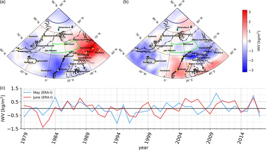
on the underlying model (Lindsay et al., 2014). Compared means. MODIS, which uses near-infrared reflectances, pro-
to the long-term climatology from ERA-Interim (Dee et al., vides valid retrievals with much lower sampling than the
2011), both May and June 2017 were slightly drier when av- others, and therefore only its monthly mean IWV product
eraging over the full region, though some areas with moister is shown for completeness. An overview of the products is
conditions are evident, e.g., northern Russia in May. For the given in Table 1.
reference sites at R/V Polarstern and Ny-Ålesund, conditions
were close to the long-term mean. The 17 radiosonde stations 2.1.1 AIRS
available in the area include both below- and above-normal
conditions. The long-term record (Fig. 1) also indicates the Launched in May 2002 on board the Aqua satellite, AIRS
strong inter-annual IWV variability even when averaged over (Aumann et al., 2003) measures radiation emitted from the
such a large area, making the detection of trends challenging. atmosphere and Earth’s surface in 2378 wavelength channels
While in the last 4 years anomalies for May and June were between 3.74 and 15.4 µm. The cross-track scanning instru-
in phase, this has not always been the case in the past. For ment has a spatial resolution of 13.5 km in nadir, decreasing
the spatial comparison of the different satellite and reanalysis to 31.5 km on the edges of the 1650 km broad swath. In this
products (Table 1), we only show the results for June 2017, paper, the AIRS Version 6 Level 2 standard product (AIRS
while the ones for May 2017 are provided in the Appendix. L2 v6 IR-Only) for orbital data with a 45 × 45 km horizontal
For most of the products IWV is not a directly measured resolution is used.
quantity but derived by integrating the vertical humidity pro- The AIRS water vapor profile product is based on a phys-
file. In this exercise differences between products can occur ical retrieval algorithm using AIRS IR radiances only and no
due to differences in the vertical sampling and the defini- MW information. One of the first steps is to apply a cloud
tion of the lower–upper boundary. The first point is of spe- clearing to the measured AIRS radiances. The retrievals of
cial relevance for radiosonde measurements and model pro- geophysical parameters are performed sequentially using the
files when strong vertical moisture gradients occur, e.g., dur- clear column radiances and an initial state being derived from
ing moisture inversions, which are frequent in the Arctic a neural network approach (Susskind et al., 2014). Each geo-
(Naakka et al., 2018). This effect can lead to differences be- physical parameter retrieval uses its own set of AIRS chan-
tween high-resolution radio soundings and those only using nels: for the water vapor profile retrieval, 41 channels in the
main pressure levels of several kilograms per square meter spectral ranges from 1310 to 1605 and 2608 to 2656 cm−1
for individual profiles. The second effect mainly concerns the are taken into account. IWV is directly provided in the oper-
lower boundary as a height difference between two products ational product (totH2OStd) and has been calculated by in-
can cause systematic biases and is most important in oro- tegrating over the retrieved specific humidity reported at 14
graphically structured terrain where the effective footprint of atmospheric layers between 1100 and 50 mbar.
models and satellite products causes different average eleva- An empirical error estimate is operationally provided
tions. As a rule of thumb a height difference of 100 m in the (totH2OStdErr) and is calculated from a number of predic-
presence of 5 g m−3 absolute humidity (typical maximum for tors (for details see Susskind et al., 2014). It depends strongly
the Arctic) causes an IWV difference of 0.5 kg m−2 . Simi- on the underlying surface and the presence of hydromete-
larly, synoptic pressure deviations can be problematic (Di- ors. Over the cloud-free ocean, uncertainty values are around
vakarla et al., 2006) when vertical profiles are provided on 2 kg m−2 or even lower, while they can reach more than
fixed pressure grids. 5 kg m−2 in precipitating regions. Only measurements with
the quality flag (totH2OStd_QC) Q = 0 (“highest quality”)
2.1 Satellite products and Q = 1 (“good quality”) are used in the following. Note
that when comparing IASI L2 PPFv6 and a similar IR–MW
In total, six satellite products available from polar-orbiting combined AIRS product to GNSS measurements, Roman
satellites operating in different parts of the electromagnetic et al. (2016) found a very similar performance in the Arctic.
spectrum are evaluated. Purely microwave information is
used by the Advanced Microwave Scanning Radiometer 2
https://doi.org/10.5194/amt-14-4829-2021 Atmos. Meas. Tech., 14, 4829–4856, 2021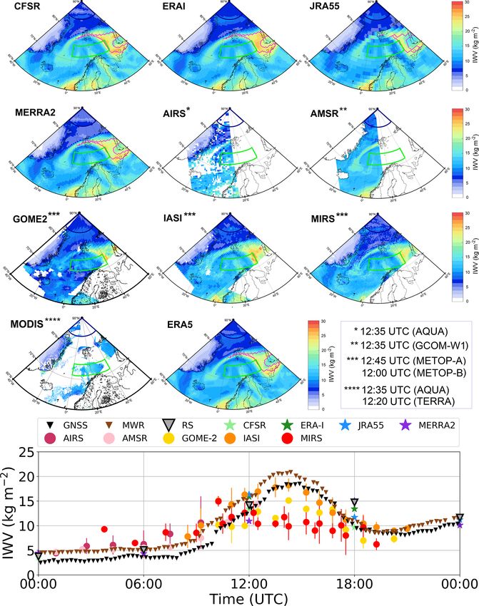
4832                                                                       S. Crewell et al.: Arctic water vapor intercomparison

Figure 1. Study area and location of reference stations together with map of IWV anomaly with respect to ERA-Interim long-term climatol-
ogy (1979–2016) for May (a) and June (b) 2017. Yellow triangles show radiosonde stations. Average sea ice margin is given as dashed black
line. Two areas studied in detail are indicated in dark blue (central Arctic) and dark green (open ocean); (c) time series of IWV anomaly
averaged over study area (60–90◦ N, 40◦ W–60◦ E) for May and June from 1979 to 2017.

Table 1. Overview of water vapor products used in this study and their nominal resolution. Note that for cross-track imagers (e.g., IASI,
MHS) the spatial resolution is highest for nadir and decreases with scan angle.

    Instrument       Platform        Product           Comments                                           Reference
                                     resolution
    AIRS             Aqua            45 km             Cloud clearing at high resolution, purely AIRS     Aumann et al. (2003)
    AMSR-2           GCOM-W1         ∼ 20 km           All-sky, ERA-Interim as a priori                   Scarlat et al. (2017)
    GOME-2           Metop-A,B       40, 80 × 40 km    No external data in retrieval                      Noël et al. (2008)
    IASI             Metop-A,B       12 km (nadir)     Combined with AVHRR and MHS                        August et al. (2012)
    MIRS             Metop-A,B,      16 km (nadir)     Variational algorithm, no NWP forecast involved    Boukabara et al. (2011)
                     NOAA-18,19                        Same core software for all satellites
    MODIS            Aqua, Terra     1 km              Only daytime over reflective surfaces              Gao and Kaufman (2003)
    Reanalysis       Producer        Original          Assimilation                                       Reference
                                     resolution
    CFSR             NCEP            ∼ 38 km           AIRS, limited AMSU-B/MHS, IASI                     Saha et al. (2014)
    ERA5             ECMWF           ∼ 30 km           All-sky microwave radiances                        Hersbach et al. (2020)
    ERA-Interim      ECMWF           ∼ 79 km           AMSU-B/MHS, SSM/I, SSMIS                           Dee et al. (2011)
    JRA-55           JMA             1.25 × 1.25◦      AMSR-2, AMSU-B/MHS, SSM/I, SSMIS                   Kobayashi et al. (2015)
    MERRA2           NASA            ∼ 55 km           AMSU-B/MHS                                         Gelaro et al. (2017)

Atmos. Meas. Tech., 14, 4829–4856, 2021                                                  https://doi.org/10.5194/amt-14-4829-2021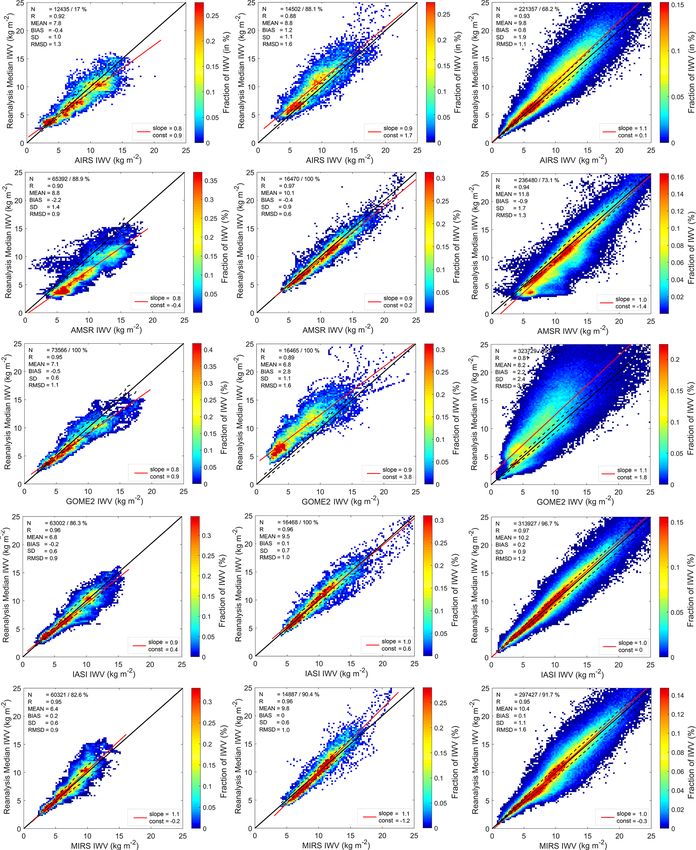
S. Crewell et al.: Arctic water vapor intercomparison                                                                        4833

2.1.2   AMSR                                                        (Metop) satellites, with Metop-A (launched October 2006)
                                                                    and Metop-B (launched September 2012) in orbit during the
The Advanced Microwave Scanning Radiometer 2 (AMSR2)                time period of ACLOUD/PASCAL. The spatial resolution of
is the successor of the AMSR and AMSR-E instruments                 the used GOME-2 measurements is 40 × 40 km for Metop-A
and has been in operation since May 2012 on the GCOM-               and 80 × 40 km for Metop-B with a swath width of 960 and
W1 satellite from the Japan Aerospace Exploration Agency            1920 km, respectively.
(JAXA). The low-frequency imager has a conical scan ge-                The GOME-2 total column water vapor (TCVW, here
ometry with an incidence angle of 55◦ . The instrument mea-         called IWV) data have been derived with the air-
sures microwave emissions from the Earth’s surface and at-          mass-corrected differential optical absorption spectroscopy
mosphere in 14 channels at 7 different frequencies (6.9, 7.3,       (AMC-DOAS) algorithm (Noël et al., 2008, and references
10.65, 18.7, 23.8, 36.5 and 89 GHz) in vertical and horizontal      therein). The AMC-DOAS product is defined as the total col-
polarizations (JAXA, 2016). The AMSR2 Level L1R data set            umn water vapor with respect to mean sea level, so it will be
(JAXA, 2013) used contains spatially consistent microwave           typically too high for high surface elevation (which is the
brightness temperature observations resampled to the respec-        case for Greenland). The AMC-DOAS method is applied to
tive footprint sizes of the 6.9, 10.65, 23.8 and 36.5 GHz chan-     sun-normalized earthshine radiance spectra in the range be-
nels using the Backus–Gilbert method (Backus and Gilbert,           tween 688 and 700 nm, where both water vapor and molec-
1968).                                                              ular oxygen (O2 ) absorb. Only data for solar zenith angles
   Integrated water vapor is acquired by an optimal estima-         less than 88◦ are used, which is no problem in this season,
tion method (OEM) (Scarlat et al., 2017). It retrieves en-          i.e., polar day. Like in standard DOAS methods, the total
sembles of surface and atmospheric parameters in the Arc-           amount of H2 O is in principle derived from the depths of the
tic, and it can use input from all AMSR2 channels. For this         observed differential absorption features. In addition, AMC-
study a special configuration of the OEM was implemented            DOAS also (i) accounts for non-linearity (saturation effects)
which uses all channels between 18.7 and 89 GHz, resam-             resulting from the strong and highly variable spectral struc-
pled to the footprint of the 23.8 GHz channels. This input          tures of water vapor which are not resolved by GOME-2
combination was chosen because it provides a better reso-           and (ii) performs a correction for the observed light path (air
lution / sensitivity ratio than using the full AMSR2 channel        mass correction) of the retrieved water vapor total columns
suite. The method inverts the Wentz radiative transfer for-         using O2 spectral structures. The air mass correction factor
ward model (Wentz and Meissner, 2000) to find a set of geo-         is also used as an a posteriori quality check, i.e., retrieved
physical parameters that best fit the measured satellite top-of-    data which require too large of a correction are filtered out.
atmosphere (TOA) brightness temperatures. Seven geophysi-           This also removes most of the cloudy scenes, but an influence
cal parameters, i.e., integrated water vapor, liquid water path,    of remnant clouds shielding part of the water vapor columns
wind speed, sea surface temperature, ice surface tempera-           may still be present. This may result in AMC-DOAS water
ture, total ice concentration and multiyear ice fraction, are re-   vapor columns which are sometimes slightly too low.
trieved simultaneously by the OEM. The retrieval results are           The AMC-DOAS method products do not rely on external
of the same spatial resolution as the lowest-frequency chan-        data (e.g., actual meteorological fields or cloud information
nel involved, i.e., 20 km.                                          from other sensors or products) and therefore provide a com-
   Surface emissivity is needed to initialize the forward           pletely independent data set. However, not making use of, for
model and implement the atmospheric correction. For the             example, available a priori information also limits the accu-
open ocean, the surface emissivity is simulated by the for-         racy of the products. In this study, we use GOME-2 AMC-
ward model using physical temperature, salinity and surface         DOAS water vapor data V0.5.5 with the recommended fil-
roughness. For sea ice, the surface emissivity is a linear com-     ters (maximum solar zenith angle of 88◦ , minimum air mass
bination of ice type areal fraction and channel-specific em-        correction factor of 0.8) applied. The precision of the AMC-
pirical monthly emissivities from Mathew et al. (2009). For         DOAS GOME-2 products (estimated from the fit residuals)
water vapor, the 23.8 GHz water vapor absorption channels           is usually better than 0.5 kg m−2 at high latitudes; however,
and the 89 GHz show the highest sensitivities and informa-          systematic errors (especially due to non-filtered-out clouds
tion content. Uncertainties for IWV are at a 2 to 3 kg m−2          and currently unconsidered surface elevation) may in general
level depending on the ice concentration (Scarlat et al.,           reach up to 5 kg m−2 , but these are considered to be some-
2017, 2020). Hereafter this product is called AMSR.                 what smaller for the conditions of the present study (low
                                                                    IWV, mostly ocean).
2.1.3   GOME-2
                                                                    2.1.4   IASI L2 PPFv6
The Global Ozone Monitoring Experiment 2 (GOME-2)
is a grating spectrometer covering the spectral range be-           The Infrared Atmospheric Sounding Interferometer (IASI)
tween about 240 and 780 nm (Munro et al., 2016). It is part         (Blumstein et al., 2004) is a hyperspectral sounder operat-
of the payload of the series of Meteorological Operational          ing in the thermal infrared. It measures between 645 and

https://doi.org/10.5194/amt-14-4829-2021                                             Atmos. Meas. Tech., 14, 4829–4856, 2021
4834                                                                      S. Crewell et al.: Arctic water vapor intercomparison

2700 cm−1 , with a spectral resolution of 0.5 cm−1 . The ob-        (Boukabara et al., 2011). The MIRS IWV product has a reso-
servations are acquired in a step-and-stare mode across the         lution of 16 km at nadir and a swath width of about 2000 km.
satellite track. The swath is approximately 2200 km wide.              MIRS provides retrievals from several different satellites.
Each field of regard is composed of 2 × 2 instantaneous fields      Here, only retrievals from the sounding instruments (AMSU,
of view (IFOVs) within a 50 km × 50 km box. The IFOV                MHS) on board Metop-A, Metop-B, NOAA-18 and NOAA-
footprints are circular, with a diameter of 12 km at nadir.         19 are used. We chose to omit the Global Precipitation Mea-
They grow elliptical and grow up to 40 km in the major              surement Microwave Imager as it does not cover the cen-
axis at the swath edge. Like GOME-2, the IASI flies on              tral Arctic and would only provide information below 65◦ N.
board the Metop satellites in a sun-synchronous orbit on the        Furthermore, during the end of June 2017, retrievals from the
09:30 UTC descending node. At mid and lower latitudes, the          F17 and F18 satellites showed a sudden drop in performance
IASI revisits the same location twice per day. More frequent        and were excluded from the analysis as well. By analyz-
overpasses at high latitudes are made possible because of the       ing microwave-imager-based wind products over the ocean,
polar orbit.                                                        Robertson et al. (2020) also observed quality issues related
   The IASI flies with two microwave companions, the Ad-            to recent observations by SSMIS and concluded that the cal-
vanced Microwave Sounding Unit (AMSU) and the Mi-                   ibration of recent SSMIS observations needs to be carefully
crowave Humidity Sounder (MHS) (Klaes et al., 2007).                assessed. We only use MIRS retrievals with a quality flag of 1
The MHS is a cross-track sounder incorporating higher               (mirs_good). The data are checked to avoid duplicates which
microwave channels, i.e., 89, 157, 190.3, 183.3 ± 3.0 and           exist due to the overlap of orbits in the individual files. We
183.3 ± 1.0 GHz. Temperature and humidity profiles belong           calculate the daily means from the orbital data.
to the suite of geophysical parameters retrieved and dis-
seminated in near-real time by the EUropean organization            2.1.6    MODIS
for the exploitation of METeorological SATellites (EUMET-
SAT) central facility (August et al., 2012). The retrieval is in-   The Moderate Resolution Imaging Spectroradiometer
dependent from numerical weather forecasts and solely relies        (MODIS) provides daytime IWV based on near-infrared
on the observations. It is performed in two steps, first with a     (NIR) measurements (Gao and Kaufman, 2003). The IWV
statistical retrieval, trained with a machine learning approach     is retrieved by using the ratio of NIR water-vapor-absorbing
and real observations, followed by an optimal estimation re-        channels and atmospheric window channels. From this water
trieval scheme in cloud-free pixels. The statistical retrieval      vapor transmittance the IWV is derived with an accuracy
is operative in nearly all-sky, while the optimal estimation        of 5 %–10 %, making use of theoretical radiative transfer
is only invoked in cloud-free pixels to refine temperature and      calculations and a look-up-table procedure. IWV collection
humidity profiles further. The cloud mask is inferred from the      6 products are available for the MODIS instruments on board
IASI observations, supported by the collocated scene anal-          the afternoon and morning polar-orbiting satellites Aqua
ysis with the companion imager instrument, the Advanced             and Terra separately. Combined, they provide a near-global
Very High Resolution Radiometer (AVHRR). Since version              coverage twice a day. We make use of the Level 3 monthly
6 of the IASI L2 processor operated at EUMETSAT, the first-         mean products, MYD08_M3 (Aqua) and MOD08_M3
step all-sky retrieval exploits the observations from the IASI,     (Terra). The spatial resolution of MODIS NIR IWV products
AMSU and MHS in synergy. The total column water vapor is            is 1 km at nadir for the orbital files and 1◦ for the monthly
integrated from the retrieved profiles and has been subject to      means.
dedicated validation against ground-based GNSS IWV mea-                Level 2 orbital data (MYD05_L2 (Aqua) and MOD05_L2
surements (Roman et al., 2016). The utilization of microwave        (Terra)) are exemplarily shown for 1 d, highlighting the low
measurements in addition to the IASI enables accurate re-           data availability of MODIS IWV in many parts of the Arctic
trievals in most cloudy conditions, where clouds otherwise          regime. This is due to the inability of MODIS to penetrate
prevent accurate sounding down to the surface with infrared-        clouds, which have a high occurrence over the Arctic and
only retrievals.                                                    subarctic ocean (Mioche et al., 2015), and the need for highly
                                                                    reflective surfaces. In case of a cloudy regime, only the IWV
2.1.5   MIRS                                                        above the cloudy layer(s) can be retrieved. Therefore, daily
                                                                    means of IWV by MODIS are not used, and only the monthly
The Microwave Integrated Retrieval System (MIRS) IWV                means are shown in our investigations.
product from the National Oceanic and Atmospheric Admin-
istration (NOAA) is derived for different microwave satellite       2.2     Reanalyses
instruments during all weather conditions and over all sur-
faces in near real time. A fast 1D-Var algorithm is used for        The same four modern global atmospheric reanalyses as
the retrieval in which the first guess is a multi-linear regres-    in Rinke et al. (2019) are used in this study, i.e., the Na-
sion algorithm, developed by collocating satellite measure-         tional Centers for Environmental Prediction (NCEP) Cli-
ments with numerical weather prediction (NWP) analyses              mate Forecast System Reanalysis (CFSR; Saha et al., 2014);

Atmos. Meas. Tech., 14, 4829–4856, 2021                                              https://doi.org/10.5194/amt-14-4829-2021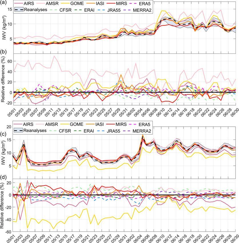
S. Crewell et al.: Arctic water vapor intercomparison                                                                        4835

the European Centre for Medium-Range Weather Fore-                regression algorithm for the AWIPEV and Polarstern mea-
casts (ECMWF) interim reanalysis (ERA-Interim, here-              surements. HATPRO provides IWV during all weather con-
after ERAI; Dee et al., 2011); the Japanese Meteorologi-          ditions except for cases when the radome of the instrument
cal Agency (JMA) 55-year Reanalysis (JRA-55; Kobayashi            is wet, e.g., due to precipitation. The accuracy is estimated to
et al., 2015); and the NASA Global Modeling and Assim-            be about 0.5 kg m−2 .
ilation Office (GMAO) Modern-Era Retrospective Analysis              Continuous measurements by the MWR and GNSS are
for Research and Applications, version 2 (MERRA2; Gelaro          able to capture the temporal variability rather well and com-
et al., 2017). Due to the lack of any reference data and in or-   plement the radiosondes (Fig. 2). Compared to the radioson-
der to compare with Rinke et al. (2009), the median of the        des, MWR (GNSS) IWV has a bias of −0.3 (−1.2) kg m−2
four reanalyses is taken as reference.                            and an RMSD of 0.5 (1.3) kg m−2 at Ny-Ålesund. Conse-
   Furthermore, we explore the performance of the next-           quently, GNSS is by lower than the MWR by 0.6 kg m−2 ,
generation ECMWF reanalysis, ERA5 (Hersbach et al.,               which is also well visible in the time series of 1 individual
2020), which has a higher spatial resolution than all other       day (Fig. 4). It is worth noting that these skill scores de-
global reanalyses except CFSR (Table 1). For our studied          rived for the ACLOUD period are well in line with those
period of 2017, the CFSv2 operational analysis is used,           calculated over the period from 2015 to 2018 (not shown),
which has a similarly high resolution (∼ 27 km) as ERA5           indicating that the biases are rather stable. The SDs between
(∼ 30 km). Furthermore, CFSv2 involves a coupling of at-          the three different instrument types are lower than 0.8 kg m−2
mosphere and ocean and an interactive sea ice model.              and thus make them well suited for the following evaluation
                                                                  of the spatial products.
2.3   Reference IWV measurements

In order to evaluate the quality of the spatial products, we      3   Matching satellite and reanalysis data with reference
make use of radiosondes and ground-based remote sens-                 IWV measurements
ing by GNSS and by MWR at selected stations (Fig. 1).
Radiosondes were taken from the Integrated Global Ra-             All satellites considered have sun-synchronous orbits with
diosonde Archive (IGRA) (Durre et al., 2006), with the ex-        orbit durations of about 100 min. For 2017, GOME-2, IASI
ception of the soundings from R/V Polarstern, available in        and MIRS observations are available from the Metop-A and
Schmithüsen (2017). For Ny-Ålesund, the accuracy of the           Metop-B satellites, while the AMSR and AIRS are only on
lower vertically resolved IGRA profiles was checked by            board one satellite, reducing their number of samples. Fig-
comparing all 143 ascents with the high-resolution data (Ma-      ure 3 illustrates the excellent sampling of the polar orbiters
turilli, 2017a, b), yielding an excellent agreement with a root   at high latitudes and the complementarity of the morning
mean square deviation (RMSD) of 0.1 kg m−2 . During the           (Metop) and afternoon (NOAA) orbit, providing nearly con-
ACLOUD/PASCAL campaigns, RS92 (RS41) radiosondes                  tinuous sampling over two-thirds of the day. Nevertheless
were launched at R/V Polarstern (Ny-Ålesund) every 6 h            sampling strongly depends on the longitude, and it becomes
(00:00, 06:00, 12:00, 18:00 UTC synoptic times). By default,      clear that good matching with the synoptic launch times of
the data were transmitted to WMO’s Global Telecommunica-          radiosondes is often not possible, especially for the eastern
tion System (GTS) and were thus available for assimilation        regions and the launch time at 00:00 UTC.
in NWP products and atmospheric reanalyses.                          The satellite IWV products were all provided as orbital
   At Ny-Ålesund (Svalbard), the delay of the GNSS signal         data on a pixel basis. For the intercomparison with refer-
between the satellite and the ground stations is used to derive   ence data, all pixels with valid IWV retrievals in a radius of
IWV. Due to the use of rather low microwave frequencies,          50 km around the individual stations (Fig. 1) were extracted.
all-weather measurements can be conducted. The data were          As an example, Fig. 2 shows the good temporal sampling of
processed by the GeoForschungsZentrum Potsdam using the           satellite and reference (MWR, GNSS, radiosonde) measure-
European Plate Observing System (EPOS) software with a            ments over the full 2-month period for Ny-Ålesund and the
temporal resolution of 15 min and an accuracy of 1–2 kg m−2       2-week time period for the ice embarkment of the R/V Po-
(Ge et al., 2006; Gendt et al., 2004).                            larstern close to 81◦ N. During the shorter period it can be
   Continuous time series with sub-minute temporal resolu-        seen that the overpasses by Metop-A and Metop-B, which
tion are available from MWR, i.e., the Humidity And Tem-          host GOME-2, the IASI and the MHS, cover the time period
perature Profiler (HATPRO; Rose et al., 2005) operated on         between roughly 08:00 and 18:00 UTC rather well for these
board the R/V Polarstern (Griesche et al., 2020) and at Ny-       two reference sites (cf. also Fig. 3), while the AMSR mea-
Ålesund (Nomokonova et al., 2019b). Herein, IWV is re-            sures in the first half of the day (Fig. 2). The MIRS product
trieved from measurements along the 22.235 GHz water va-          covers the widest range as in addition to the Metop satellites
por absorption line by a linear regression algorithm following    also NOAA-18 and NOAA-19 are used.
Löhnert and Crewell (2003). A decade-long training data set          In order to compare the satellite measurements with refer-
of GRUAN sondes from Ny-Ålesund has been used in the              ence data, different criteria are used: (i) the highly temporally

https://doi.org/10.5194/amt-14-4829-2021                                            Atmos. Meas. Tech., 14, 4829–4856, 2021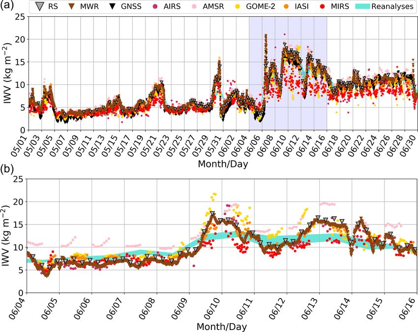
4836                                                                         S. Crewell et al.: Arctic water vapor intercomparison

Figure 2. Time series of reference data (GNSS, MWR, radiosonde (RS)), reanalyses and satellites (see legend for explanation of symbols) at
the two ACLOUD central sites Ny-Ålesund (a) and the R/V Polarstern ice camp (b). The time period of the ice camp is indicated in blue in
the time series for Ny-Ålesund. Note that GNSS is not available for Polarstern. The cyan shaded area indicates the minimum and maximum
values of the reanalyses.

Figure 3. Overview of satellite data sampling for a latitude band (70–80◦ N) as a function of time of day and longitude (5◦ resolution). For
each bin (1 h, 5◦ ) the total number of measurements over the 2-month period (May–June 2017) is indicated per instrument by the size of the
corresponding symbol in quantiles. The maximum number of samples per bin is about 2000 for AIRS on Aqua, 8000 for each IASI platform
and about 10 000 for the MIRS products on each satellite.

Atmos. Meas. Tech., 14, 4829–4856, 2021                                                    https://doi.org/10.5194/amt-14-4829-2021
S. Crewell et al.: Arctic water vapor intercomparison                                                                            4837

resolved ground-based MWR data are averaged to 15 min                IWV (and integrated vapor transport) typically associated
means to match the GNSS measurements. Their temporally               with the pre-cold frontal zone of some (but not all) extra-
closest measurement to the radiosonde synoptic time is used          tropical cyclones. The ARs reaching polar regions stretch
for comparisons. (ii) A time window of ±30 min with respect          from lower latitudes and can gain the majority of their mois-
to the radiosonde time is used to identify corresponding satel-      ture in subtropical latitudes (Terpstra et al., 2021). ARs have
lite measurements. Note that a larger window length of ±1 h          also been associated with several cyclones, helping the mois-
does not drastically enhance the number of matched samples           ture supply within the same AR structure (Sodemann and
for the radiosondes due to the fixed launch times at most sta-       Stohl, 2013). In the polar regions ARs are often associated
tions. (iii) All IWV satellite measurements with a center pixel      with moisture inversions showing maxima in specific humid-
location within a 50 km circle around the location of the ref-       ity between 800 and 900 hPa (Gorodetskaya et al., 2020).
erence site are used to calculate mean IWV and its SD. The           Here we choose the AR event from 6 June 2017 at 12:00 UTC
same exercise has been performed for a larger search radius          to illustrate the capabilities of the different products (Fig. 4).
of 100 km to check the sensitivity. (iv) To eliminate outliers,      Note that this is only one out of three AR events that occurred
only IWV values between 0 and 30 kg m−2 are used, which              during ACLOUD/PASCAL documented in detail by Viceto
is sensible as IWV varies between 3 and 22 kg m−2 for the            et al., (submitted). By definition reanalyses provide infor-
Ny-Ålesund and R/V Polarstern sites (Fig. 2). While we are           mation across the full region, revealing the maximum IWV
aware that most satellite retrievals work best over ocean sur-       of about 25 kg m−2 west of Novaya Zemlya, from where an
faces (well-characterized microwave emissivity) and are af-          elongated band of IWV stretches westward, passing Svalbard
fected by differences in orography, we consciously use all           and dissolving north of Iceland with extended cloudiness and
conditions for our assessment as we aim at a climatologically        convective precipitation. As the data are shown here in their
sound data set. In order to estimate the influence of orogra-        original resolution, differences between reanalyses with re-
phy and surface emissivity, all measurements were classified         spect to gradients, coastal features and maximum IWV are
according to their position over water or land. This is for ex-      evident, showing the better representation of small-scale fea-
ample of interest for Ny-Ålesund, with a station elevation of        tures in the high-resolution ERA5 reanalysis.
11 m, which is located in a fjord surrounded by mountains up            The temporally closest Metop satellite overpass provid-
to 550 m height.                                                     ing GOME, IASI and MIRS products is on the descend-
   For maps of daily and monthly IWV, the reanalysis                 ing branch of the orbit, while Aqua (AIRS) and GCOM-
products were interpolated to the ERA-Interim grid with              W1 (AMSR) are on an ascending one (Fig. 4). The indi-
0.75◦ × 0.75◦ resolution. All orbital satellite data for a day       vidual orbits of the satellite products demonstrate the differ-
are assigned to the same 0.75◦ × 0.75◦ latitude–longitude            ent swath widths as well as the limitations of the products.
grid spanning the study area. The daily means are calcu-             The AIRS L2 v6 IR-Only product shows the largest spatial
lated as the arithmetic mean per grid cell, using only mea-          gaps due to the limitation of infrared measurements in the
surements which fulfill the quality criteria (Sect. 2.1). Due to     presence of clouds and precipitation. AMSR low-frequency
the different satellite orbits, sampling differs for the different   microwave information is also available in cloudy regions,
products (see above). Note that due to the meridian conver-          but due to the complex emissivity over land only measure-
gence, this means that at 70◦ N, the resolution along the lati-      ments over the ocean and sea ice are provided. GOME-2
tude circle is only 24 km, while it is 83 km in the meridional       provides retrievals over all surfaces, but cloud disturbances
direction.                                                           lead to data gaps close to Svalbard and north of Iceland.
                                                                     For the latter region, MIRS, which retrieves several param-
                                                                     eters simultaneously, indicates precipitation. Note that due
4     Results                                                        to the dominance of the precipitation signal, the information
                                                                     on water vapor can be obscured for heavy rain events. IASI
4.1    Direct comparisons of satellite/reanalysis with               L2 PPFv6 and MIRS, which mitigate cloud influence by the
       reference data                                                use of microwave radiances in their retrieval schemes, have
                                                                     nearly complete coverage. As already mentioned, MODIS
The ACLOUD/PASCAL campaign offers a wide range of                    only provides rather limited information as it can derive IWV
IWV conditions to investigate the performance of IWV prod-           only under cloud-free conditions over strongly reflective sur-
ucts. The time series at Ny-Ålesund (Fig. 2) first shows             faces.
an unusual dry (and cold) phase, followed by an unusual                 The daily time series of the MWR at Ny-Ålesund
wet (and warm) period (30 May–12 June) connected with                (Fig. 4, bottom) shows that IWV rapidly increases by
high IWV variability, as already described by Knudsen et al.         about 15 kg m−2 within only 5 h, reaching its peak value of
(2018). Afterwards normal conditions prevailed. Further it           22 kg m−2 around 14:00 UTC before declining again with
reveals several IWV peaks (Fig. 2), of which three were iden-        similar speed but arriving at a higher level (10 kg m−2 ).
tified as ARs following the definition by Gorodetskaya et al.        The ground-based MWR agrees well with the radiosondes
(2014, 2020). ARs are narrow corridors of anomalously high           launched during that day, with the exception of 18:00 UTC,

https://doi.org/10.5194/amt-14-4829-2021                                               Atmos. Meas. Tech., 14, 4829–4856, 2021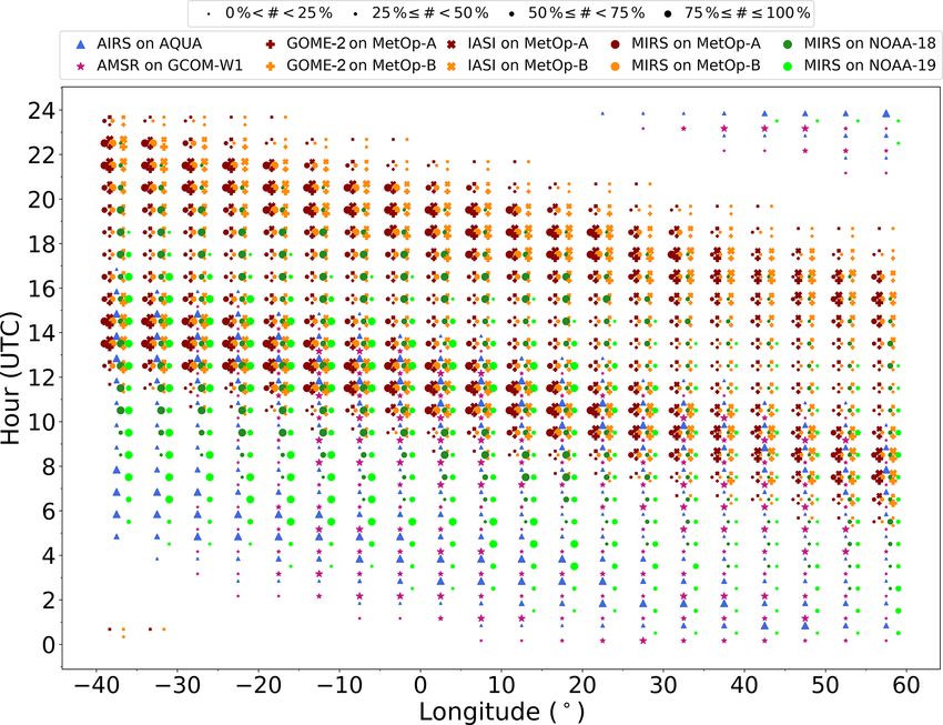
4838                                                                        S. Crewell et al.: Arctic water vapor intercomparison

Figure 4. Illustration of the AR event on 6 June 2017 as provided by four different reanalyses at 12:00 UTC and instantaneous satellite
measurements (closest orbit in time). The magenta line depicts the region where IWV is higher than an IWV threshold based on the saturated
IWV and an AR coefficient (Gorodetskaya et al., 2014) using ERA-Interim reanalysis. For the remaining reanalysis data sets, the line was
interpolated from ERA-Interim. The central Arctic (dark blue) and open-ocean (green) regions are marked. Bottom: time series at Ny-Ålesund
for 6 June 00:00 UTC to 7 June 00:00 UTC from reference data, reanalyses and satellite measurements within 50 km of the site.

which could be caused by the drift of the radiosonde across            in the movement of the AR. Looking at the satellite prod-
the strong IWV gradient. GNSS and MWR have a slight mis-               ucts shows an even larger spread among the measurements:
match in the diurnal cycle that might be due to the slant path         the AMSR, which has eight overpasses over Ny-Ålesund
between GNSS satellites and the ground receiver or problems            between 01:00 and 13:00 UTC, agrees very well with the
in the derivation of the mean weighted temperature used in             ground-based MWR before the arrival of the AR. During this
the GNSS retrieval (Morland et al., 2009). Generally, it be-           time also little variability between pixels within the 50 km ra-
comes clear that dense temporal and spatial sampling with              dius is observed, which increases strongly with the arrival of
high resolution is necessary to characterize such an event.            the AR. IASI L2 PPFv6 provides the best agreement for this
   The time series during the AR event (Fig. 4, bottom) re-            case, while GOME-2 and MIRS strongly underestimate the
veals differences of up to 6 kg m−2 at 12:00 UTC between               AR maximum. In fact, MIRS seems to have difficulties in
MERRA2 and JRA-55, which is likely due to mismatches                   retrieving higher IWV values at all, as also indicated in the

Atmos. Meas. Tech., 14, 4829–4856, 2021                                                  https://doi.org/10.5194/amt-14-4829-2021
S. Crewell et al.: Arctic water vapor intercomparison                                                                          4839

moist June period (Fig. 2). Consistently with the orbit char-           When considering all other radiosonde stations together
acteristics of the satellites (Fig. 3), towards the end of the day   (Fig. 5, right column; Table A1; for locations of stations see
no satellite matches can be found for Ny-Ålesund.                    Fig. 1), one has to take caution because the different orbit
   To quantitatively assess the accuracy of the IWV prod-            characteristics together with the fixed launch times produce
ucts, in a first step pairs between radiosonde measurements          different sets of matched stations for the different products
and corresponding products which fulfill the matching crite-         (Fig. 3). Because MIRS makes use of four different satellites,
ria (Sect. 3) are compiled (Fig. 5), and skill scores, i.e., bias,   most samples (914) are found. However, MIRS is clearly the
correlation coefficient (r), RMSD and SD (i.e., the bias-            product revealing the strongest scatter. This is not necessarily
corrected RMSD), are computed. For R/V Polarstern (Fig. 5,           due to the quality of the satellite product but might arise from
left column) only few matched samples (between 17 and 32)            the consideration of different samples. NOAA-19 has several
are available due to the limited deployment time. IASI L2            matches with Russian RS stations, while these are rare for
PPFv6 retrievals can clearly be identified, showing the best         Metop satellites. For Russian RS stations, a slope parame-
performance with the lowest bias (−0.2 kg m−2 ), highest cor-        ter lower than 1 indicates an overestimation of MIRS, which
relation (0.98) and lowest SD (0.9 kg m−2 ). Each individual         could be due to problems with surface emissivity, but an un-
radiosonde match is an average of about 10 individual pix-           derestimation of IWV by the RS can also not be excluded.
els, and their low variation indicates relatively homogeneous        On the other hand, RS stations in Greenland and northern
conditions around the site. This is also seen by the AMSR,           Scandinavia mainly show slopes larger than 1, indicating an
which has as well a rather low SD (0.9 kg m−2 ) but is affected      underestimation of MIRS. The use of different radiosonde
by a strong bias (3.2 kg m−2 ).                                      sensors in different countries or regions is known to result
   At Ny-Ålesund (Fig. 5, middle column), where more than            in an uneven distribution of temperature and humidity biases
twice as many matches are available, the AMSR shows                  across geopolitical borders (Soden and Lanzante, 1996; Ho
the highest correlation (0.99) and lowest SD (0.7 kg m−2 )           et al., 2017; Ingleby, 2017). With a correlation of 0.96, SD
followed by IASI L2 PPFv6 (r = 0.97, SD = 1.1 kg m−2 ).              of 1.29 kg m−2 and RMSD of 2.21 kg m−2 , IASI L2 PPFv6
Interestingly, the bias of the AMSR is strongly reduced              again shows the best performance of all satellite products.
(0.88 kg m−2 ) compared to the ice floe region at R/V Po-            While the scatter is much lower than in the case of MIRS,
larstern, indicating an emissivity issue for sea ice. IASI L2        the same trend with respect to over- or underestimation for
PPFv6 shows a negative bias of −0.7 kg m−2 , which can be            different stations can be seen. Detailed statistics for all in-
explained by the orography around the launch site, as ex-            dividual radiosonde stations separately are given in the Ap-
pressed by the reduction in the bias to −0.1 kg m−2 when             pendix (Table A1). Note that a direct comparison between
only pixels above water are considered. Note that no distinct        the radiosonde measurements and reanalyses has not been
changes in the other scores occur. The AIRS L2 v6 IR-Only            pursued as the radiosondes are assimilated into reanalyses.
product shows a weaker performance for both sites, with SD
being about 0.5 kg m−2 higher than for IASI L2 PPFv6. This           4.2   Assessment of daily mean data
indicates the benefit of the different IASI retrieval strategy,
e.g., individual pixels, inclusion of microwave information.         With the uncertainty in the individual satellite measurements
   The performance of GOME-2 substantially degrades for              addressed by the direct intercomparison, we now aim to in-
IWV values above 10 kg m−2 , leading to much higher SDs at           vestigate the suitability of the satellite products for climate
R/V Polarstern (1.6 kg m−2 ) and Ny-Ålesund (1.8 kg m−2 )            studies. To better understand how uncertainties are trans-
than shown by AIRS L2 v6 IR-Only, AMSR and IASI L2                   ferred, we first compile daily mean values from orbital data,
PPFv6. Considering only water surfaces even slightly wors-           which are then aggregated to monthly means (cf. Sect. 4.3).
ens the scores (not shown). GOME-2 and MIRS show a sim-              Assessing the quality of these products with reference mea-
ilar correlation (0.90) for both sites. MIRS, which has the          surements is only possible at sites with continuous ground-
highest number of matches per individual radiosonde, re-             based measurements, reducing the data set notably. There-
veals a strong underestimation for IWV values higher than            fore, in order to better identify the differences between the
about 10 kg m−2 for both R/V Polarstern as well as for Ny-           products, we look at anomalies with respect to the median of
Ålesund, where nearly 100 radiosondes are compared. This             the four classical reanalyses (CFSR, ERA-Interim, JRA55,
results in a slope in the regression of 1.44 (1.64) for R/V          MERRA2). In case of random noise, a distinct reduction in
Polarstern (Ny-Ålesund), which leads to a much narrower              uncertainty due to averaging should occur, while systematic
retrieved IWV frequency distribution than measured by ra-            errors should become more pronounced. In addition, the ir-
diosondes, thus underestimating IWV variability. For MIRS,           regular sampling of satellite data can introduce errors, which
the scores improve when only water surfaces and a larger             will depend on the prevailing weather conditions.
search radius (100 km) are used; i.e., correlation increases            The AR event of 6 June 2017 with high IWV contrasts is
from 0.90 to 0.95, and SD reduces from 2.3 to 1.6 kg m−2             used to study the differences between IWV products now on
(not shown).                                                         a daily mean basis. Compared to the snapshot at 12:00 UTC
                                                                     (Fig. 4), the AR is smoothed in the reanalysis median over the

https://doi.org/10.5194/amt-14-4829-2021                                               Atmos. Meas. Tech., 14, 4829–4856, 2021
4840 S. Crewell et al.: Arctic water vapor intercomparison Figure 5. Scatterplots for radiosondes launched at the Polarstern (left column) and Ny-Ålesund (middle column) and for all other radiosonde stations (right column) with corresponding (±30 min and 50 km radius) satellite measurements (from top to bottom row: AIRS L2 v6 IR- Only, AMSR, GOME-2, IASI L2 PPFv6, MIRS) above all surfaces. All satellite pixels falling into this criterion have been averaged, and their SD is indicated by the width of the line. The number of averaged pixels is indicated by color for the first two columns only. Atmos. Meas. Tech., 14, 4829–4856, 2021 https://doi.org/10.5194/amt-14-4829-2021
S. Crewell et al.: Arctic water vapor intercomparison                                                                            4841

Figure 6. Relative difference in the daily means of the reanalyses and satellite products to the reanalysis median (CFSR, ERA-Interim,
JRA-55, MERRA2; lower right plot) for 6 June 2017. The green line indicates the sea ice edge from AMSR sea ice data. The central Arctic
(dark blue) and open-ocean (green) regions are marked.

full day but is still visible (Fig. 6). Differences between re-       reanalysis ERA5 (not part of the reanalysis median) substan-
analyses are around 10 %, with higher deviation along coast-          tially differs from the heritage product ERAI, though some
lines and strong orography that can easily be explained by            similarities such as the positive (moist) difference over sea
differences in their original resolution. In that sense, it is not    ice appear.
a surprise that CFSR with its higher resolution shows even               In general, the deviations of the satellite products from
higher deviation in some of these areas, e.g., coast of Green-        the reanalysis median for 6 June 2017 are about a factor
land, as the orography is smoothed less, giving lower IWV at          of 2 higher than those of the reanalyses. Different to the re-
grid points with higher altitude. Over the open ocean, the spa-       analyses, the satellite products all have a different sampling
tial structure of the differences between the classical reanaly-      density per grid cell due to the different orbit characteris-
ses does not seem to be strongly related to the AR shape, with        tics (Fig. 3). Due to their orbit for these polar-orbiting satel-
the exception of the dry line close to 40◦ E in ERAI, which           lites, the best sampling globally occurs in a band centered
might hint at differences in the data assimilation of the differ-     around 73◦ N latitude. AIRS L2 v6 IR-Only and GOME-2
ent reanalyses. Instead already on the daily scale some sys-          have the lowest number of samples, while IASI L2 PPFv6
tematic differences occur over sea ice and the ocean that will        and MIRS have around 50 individual measurements per grid
be discussed later on. Interestingly, the new high-resolution         cell. In fact IASI L2 PPFv6 and MIRS show very similar geo-

https://doi.org/10.5194/amt-14-4829-2021                                                Atmos. Meas. Tech., 14, 4829–4856, 2021
4842                                                                    S. Crewell et al.: Arctic water vapor intercomparison

graphical structures in their differences, which is no surprise        To better understand systematic features, we study two re-
as the IASI L2 PPFv6 product incorporates the microwave             gions with relatively homogeneous surface conditions over
measurements on the Metop satellites. The strong bands of           the course of the ACLOUD/PASCAL campaign (cf. Fig. 1).
positive and negative deviations along the northward extent         The first region is the high Arctic north of 84◦ N (in the fol-
of the AR, reaching up to 50 % (Fig. 6), can be attributed          lowing called “central Arctic”), where no surface reference
to sampling differences due to the fast movement of the AR.         measurements exist, and biases between reanalyses are ev-
As the reanalysis median is only computed from the 6-hourly         ident: while ERAI and ERA5 show positive deviations over
IWV values, the satellites are likely able to better capture this   the full sea-ice-covered area, CFSR and MERRA2 show neg-
development. This is supported by the similar structures evi-       ative deviations as already noted by Rinke et al. (2019). The
dent in the ERA5 daily mean product (weighting all 1h time          second area concerns the ice-free North Atlantic towards the
steps). The resemblance between ERA5 and the two satellite          Barents Sea (72–75.75◦ N, 0–40◦ E; in the following called
products (IASI L2 PPFv6 and MIRS) seems to be limited               “open ocean”).
to open-ocean surfaces, where ERA5 assimilates their data.             Over the open-ocean area, low-frequency microwave ob-
Before we move on to a discussion on systematic effects, we         servations should have the best performance due to the
want to investigate the “weather-related” averaging effects in      low and well-characterized surface emissivity. Therefore
more detail.                                                        it is no surprise that the AMSR shows the lowest SD
   During the strong AR event (Fig. 4), clearly high devia-         (0.9 kg m−2 ; Fig. 7, Table 2) compared to the reanalysis me-
tions of several kilograms per square meter between different       dian, which might also be due to its assimilation into the
products are possible if the daily mean is calculated from few      reanalyses. The same holds for MIRS and IASI L2 PPFv6
samples – but how frequently does this occur? To investigate        (with SD = 0.6 kg m−2 and SD = 0.7 kg m−2 , respectively),
the limitations due to infrequent temporal sampling we use          which incorporate higher microwave frequencies. With fre-
the continuous MWR IWV at Ny-Ålesund, which is avail-               quent low-level cloudiness over the North Atlantic, it is no
able in sub-minute resolution. The basic idea is to mimic the       surprise that the pure thermal IR (AIRS L2 v6 IR-Only;
sampling characteristics of other observation systems such as       bias = 1.2 kg m−2 , SD = 1.1 kg m−2 ) and solar spectral range
radiosonde stations or sporadic satellite overpasses. During        (GOME-2; bias = 2.8 kg m−2 , SD = 1.1 kg m−2 ) have diffi-
ACLOUD/PASCAL daily mean values calculated from the                 culties also reflected in the much poorer correlation. The dif-
four time steps such as from 6-hourly radiosonde launches           ferent behavior between the different satellite products is fur-
would give a negligible deviation on average with an SD of          ther illustrated by looking at the temporal development over
0.3 kg m−2 , but individual deviations of 1 kg m−2 or more oc-      the 2 months (Fig. 8). The AMSR, IASI L2 PPFv6 and MIRS
cur. When looking at a multiyear data set (2015–2018; not           show overall similar performances as the reanalyses, repro-
shown), no bias but an SD of 0.5 kg m−2 is present. Most of         ducing IWV day-to-day variability well, with daily means
the Arctic radiosonde stations launch sondes twice or some-         between 5 and 15 kg m−2 . In this homogeneous region, re-
times only once per day. In this case, the deviations from          analyses are highly consistent, with SDs of 0.3 to 0.4 kg m−2
the true daily mean are even worse. Generally, the SD de-           (Fig. A1). However, the reanalysis bias (Table 2) varies
pends on IWV itself, with a relative SD of 5 % and samples          between −0.7 kg m−2 (CFSR) and +0.6 kg m−2 (JRA55),
every 6 h, and degrades to 10 % if two samples (00:00 and           which might be related to differences in data assimilation
12:00 UTC) are used. Taking only the 12:00 UTC measure-             or model physics. In fact, the reanalyses differ in their dif-
ment as representative of 1 d only slightly worsens the situa-      ferences more than the three satellite products, which vary
tion, with a relative SD of 12 %.                                   between −0.4 kg m−2 (AMSR) and +0.1 kg m−2 (IASI L2
   In the comparison of the daily mean differences, several         PPFv6). Therefore one might conclude that in open-ocean
geographic features appear that point to systematic effects         areas these satellite products can be used to further improve
(Fig. 6). Consistent with the previously discussed time se-         reanalyses.
ries for R/V Polarstern (Fig. 2), the AMSR shows a positive            For the sea ice region, one can nicely see how the rather
bias over the sea ice of more than 30 %. Over sea ice, also         constant dry conditions in the central Arctic prevailing in the
GOME-2 shows a positive bias, pointing at an issue with             first half of May are changed by moisture transport from the
surface reflectivity for GOME-2 and surface emissivity for          south (Fig. 8). This transport mostly takes place by individ-
the AMSR. The positive bias of GOME-2 over Greenland is             ual events such as the AR event discussed before that results
partly due to the definition of the product that provides the       roughly in a tripling of IWV in the ACLOUD/PASCAL pe-
column above mean sea level. Due to the high elevation of           riod. The sporadic nature in the transport seems to cause a
the Greenland ice sheet, the lowest absolute IWV occurs here        larger spread between reanalyses and also satellite products
(see reanalysis median). Therefore small absolute IWV dif-          (cf. period from 10 June onward). Similar to the open ocean,
ferences lead to high relative differences (also seen by AIRS       relative differences between reanalyses are up to ±10 %. Out
L2 v6 IR-Only and IASI L2 PPFv6). MIRS shows a high                 of the satellite products, only IASI L2 PPFv6 shows similar
positive overestimation over the Russian land area, consis-         performance as reanalysis. While GOME-2 showed strong
tent with the radiosonde intercomparison.                           IWV underestimation over the dark open ocean, its perfor-

Atmos. Meas. Tech., 14, 4829–4856, 2021                                              https://doi.org/10.5194/amt-14-4829-2021
You can also read