Accounting for tropical cyclones more than doubles the global population exposed to low-probability coastal flooding - Nature
←
→
Page content transcription
If your browser does not render page correctly, please read the page content below
ARTICLE
                  https://doi.org/10.1038/s43247-021-00204-9               OPEN

                  Accounting for tropical cyclones more than doubles
                  the global population exposed to low-probability
                  coastal flooding
                  Job C. M. Dullaart 1 ✉, Sanne Muis                    1,2,   Nadia Bloemendaal           1,   Maria V. Chertova3, Anaïs Couasnon1 &
                  Jeroen C. J. H. Aerts 1,2

                  Storm surges that occur along low-lying, densely populated coastlines can leave devastating
                  societal, economical, and ecological impacts. To protect coastal communities from flooding,
1234567890():,;

                  return periods of storm tides, defined as the combination of the surge and tide, must be
                  accurately evaluated. Here we present storm tide return periods using a novel integration of
                  two modelling techniques. For surges induced by extratropical cyclones, we use a 38-year
                  time series based on the ERA5 climate reanalysis. For surges induced by tropical cyclones, we
                  use synthetic tropical cyclones from the STORM dataset representing 10,000 years under
                  current climate conditions. Tropical and extratropical cyclone surge levels are probabilistically
                  combined with tidal levels, and return periods are computed empirically. We estimate that 78
                  million people are exposed to a 1 in 1000-year flood caused by extratropical cyclones, which
                  more than doubles to 192 M people when taking tropical cyclones into account. Our results
                  show that previous studies have underestimated the global exposure to low-probability
                  coastal flooding by 31%.

                  1 Institute for Environmental Studies (IVM), Vrije Universiteit Amsterdam, Amsterdam, The Netherlands. 2 Deltares, Delft, The Netherlands. 3 Netherlands

                  eScience Center, Amsterdam, The Netherlands. ✉email: job.dullaart@vu.nl

                  COMMUNICATIONS EARTH & ENVIRONMENT | (2021)2:135 | https://doi.org/10.1038/s43247-021-00204-9 | www.nature.com/commsenv                                1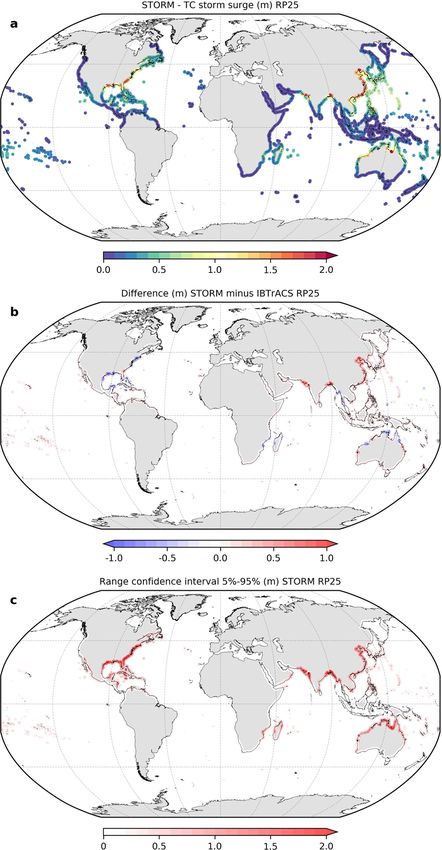
ARTICLE                                             COMMUNICATIONS EARTH & ENVIRONMENT | https://doi.org/10.1038/s43247-021-00204-9

D
         riven by strong winds and low pressures in tropical                in prior research18,26,39, our methodology contains two main
         cyclones (TCs) and extratropical cyclones (ETCs), storm            novelties. First, TC-induced and ETC-induced storm surges are
         surges may threaten coastal areas, especially when they            modeled separately using different types of meteorological forcing.
coincide with high tides1. Globally, approximately 100 million              For TCs we use synthetic TC tracks from the STORM dataset28.
people live in areas below the current high tide lines2. As a               STORM is a fully statistical model that extracts the TC char-
consequence, a substantial portion of the socio-economic activity           acteristics from any input dataset, in this case, IBTrACS
and critical infrastructure is exposed to coastal flooding3,4.               (1980–2017), and statistically resamples this to the equivalent of
Examples of recent high-impact storm surge events with their                10,000 years under the same climate scenario. For ETCs we use the
maximum surge level and overall losses include TCs Dorian                   ERA5 climate reanalysis. With ETC storm surges we refer to all
(Bahamas; 7.0 m; $5.1B)5 and Michael (United States; 4.3 m;                 surges not caused by a TC. As a result, ETCs are the main drivers
$25.0B)6 and ETCs Xaver (northern Europe; 3.5 m; $1.4B)7 and                of extremes in the ETC surge level time series, though they also
Ophelia (Ireland; 1.7 m; $1.0B)8. TCs generally form over warm              include extremes generated by other weather phenomena such as
tropical waters and affect regions such as Southeast Asia, the              depressions, anti-cyclonic storms, monsoons, and polar lows40,41.
Caribbean, and North Australia9, while ETCs dominate in the                 Second, the extreme value analysis (EVA) method consists of an
mid-latitudes and affect regions such as South America, Europe,             empirical approach based on a large sample size rather than fitting
and South Australia. In addition, there are regions that experience         extreme value distributions and extrapolating storm tide levels to
both storm systems, including the west and east coasts of Aus-              high RPs. To accomplish this, we generate stochastic storm tide
tralia (±30°S)10,11, eastern China (±35°N)12, and the east coast of         event sets based on the possible combinations of tides and surges
the United States (±40°N)13,14.                                             from TCs and ETCs. This allows for estimations of rare storm tide
   Return periods of storm tides (RPs), defined as the combina-              RPs with high statistical confidence that produce a consistent
tion of storm surge and tide, can provide highly valuable input to          global dataset with storm tide RPs. Finally, we show how the full
flood hazard and flood risk assessments15,16. RPs are often used              inclusion of TCs changes the exposure of the global population to
as design standards for the construction of coastal levees and              low-probability coastal flooding.
other flood protection measures17. On continental to global
scales, studies have used RPs to model coastal flooding18–20 and
                                                                            Results
societal risks under future scenarios of sea-level rise and socio-
                                                                            TC storm surge RPs. The 25-year return period (RP25) of TC-
economic development21–25.
                                                                            induced storm surges exceeds 2.0 m in several regions (Fig. 1a),
   All global-scale studies on storm tide RPs have inaccuracies in
                                                                            including the Yellow Sea and East China Sea (China), the Gulf of
TC-prone regions18,19,26,27. The cause of this inaccuracy is two-
                                                                            Carpentaria (Australia), the Bay of Bengal (Bangladesh), and the
fold: (1) TCs are poorly resolved due to the coarse spatial and
                                                                            gulf and east coasts of the United States. For this, we simulate TC
temporal resolution of meteorological forcing data, causing an
                                                                            storm surges by forcing the Global Tide and Surge Model
underestimation in TC intensity and, consequently, storm surge
                                                                            (GTSM)26 with 3000 years of the current climate (1980–2017)
level; and (2) in combination with the low-probability of TCs28,
                                                                            synthetic TC tracks from the STORM dataset28 (see “Methods”
the limited record length of the meteorological forcing data
                                                                            section). Subsequently, we apply the Weibull plotting position
(typically 40 years)—with ±90 TCs forming per year and only 16
                                                                            formula to the simulated TC storm surge levels and estimate RPs
of these making landfall29—means the number of TCs is too
                                                                            (Supplementary Fig. 1). To compare the STORM-based results
small to robustly estimate RPs. In addition, TCs affect a relatively
                                                                            against historical events, we force GTSM with the same TC tracks
small stretch of coastline30, which reduces the number of recor-
                                                                            that were used as input for the STORM model. These TCs are
ded TC-induced storm surges. Recent advances in climate mod-
                                                                            filtered from IBTrACS9 by selecting those TCs with maximum
eling, such as the newly developed ERA5 climate reanalysis
                                                                            wind speeds equal to or larger than 18 m s−1, that form within a
dataset, have improved the modeling of TC storm surges31.
                                                                            TC basin and within a TC season (see ref. 28 for an overview).
However, ERA5’s record length of several decades is too short for
                                                                            This amounts to 2710 historical TCs in the period 1980–2017.
a robust estimation of high RPs in TC-prone regions11,14,15.
                                                                            Differences in RP25 surge levels between STORM and IBTrACS
   To overcome these limitations, regional studies on TC storm
                                                                            are smaller than 0.25 m for 85% and 0.10 m for 67% of the output
surges have extended the historical TC record by generating
                                                                            locations prone to TCs (Fig. 1b). In the Gulf of Mexico, the east
synthetic TC tracks32–34. These synthetic TC tracks, representing
                                                                            coast of the United States, parts of northern Australia, and
thousands of years of TC activity, are generated through statistical
                                                                            Madagascar, the difference in RP25 is larger than 0.5 m. However,
resampling and modeling of observed TC tracks and intensities.
                                                                            the 90% confidence interval of STORM RP25 also exceeds 0.5 m
The main advantage of such a method is that it does not assume
                                                                            in those regions with large differences between the STORM-based
an upper tail behavior based on an extreme value fit, which can be
                                                                            and IBTrACS-based RP25 (i.e., at 24% of the output locations).
unstable with a limited sample size. Instead, low exceedance
                                                                            This suggests that at least part of the difference between the
probabilities are estimated empirically from the large set of
                                                                            synthetic and observed TCs is explained by the stochastic nature
reconstructed events. Such approaches have been applied in
                                                                            of TCs where the 38-year period of IBTrACS can contain too
places like Australia10,11, The United States35, New York13,14,
                                                                            many (or few) or too extreme (or weak) storm surge events
Tampa, Cairns, and the Persian Gulf36. More recent, global-scale
                                                                            compared to the probability of a certain TC storm surge event
studies have built on these regional approaches and developed
                                                                            based on STORM. An example of a storm surge event with a
new synthetic TC datasets, enabling RP estimates for up to
                                                                            much higher RP than 38 years is TC Sandy, which made landfall
10,000-years28,37,38 with high statistical confidence. These novel
                                                                            near New York and has an estimated storm tide RP of 260
datasets pave the way to properly account for TC-induced storm
                                                                            years14; this emphasizes the need for a long time series of TC
surges and compute more robust storm tide RPs on a global scale.
                                                                            storm surge levels in order to accurately compute RPs.
However, a global-scale study on storm tide RPs using synthetic
TC tracks has never been conducted.
   This study addresses this research gap by presenting a new               ETC storm surge RPs. The RP25 for ETC-induced storm surge
combined global dataset of TC and ETC storm tide RPs that we                levels exceeds 2.0 m along with parts of the coastline of Argentina,
call COAST-RP (COastal dAtaset of Storm Tide Return Periods).               Uruguay, Australia, and countries bordering the Arctic Ocean
Building upon the hydrodynamic modeling framework presented                 and the North Sea (Fig. 2a). To compute ETC RPs we use 38 years

2           COMMUNICATIONS EARTH & ENVIRONMENT | (2021)2:135 | https://doi.org/10.1038/s43247-021-00204-9 | www.nature.com/commsenv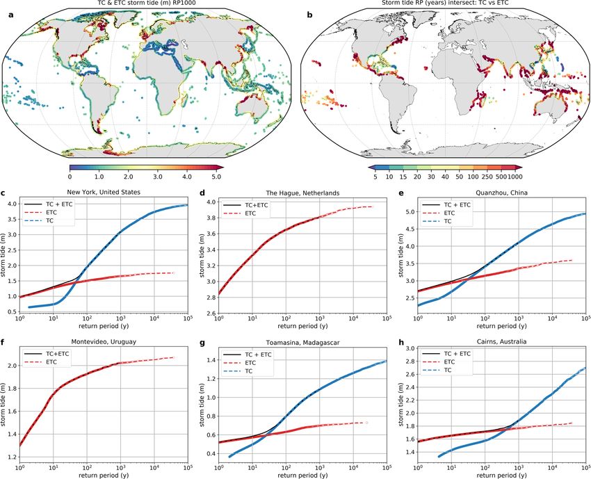
COMMUNICATIONS EARTH & ENVIRONMENT | https://doi.org/10.1038/s43247-021-00204-9                                                    ARTICLE

Fig. 1 Tropical cyclone-induced storm surge levels with a 25-year return period. The panels show the (a) STORM-based 25-year tropical cyclone storm
surge return period, (b) absolute difference (m) in TC storm surge levels between STORM and IBTrACS, and (c) the range of the 90% confidence interval
(m) of STORM. The difference in surge level is calculated by subtracting the IBTrACS-based RPs from STORM; the range of the confidence interval is
calculated as the difference between the 5th and 95th percentile.

COMMUNICATIONS EARTH & ENVIRONMENT | (2021)2:135 | https://doi.org/10.1038/s43247-021-00204-9 | www.nature.com/commsenv                           3
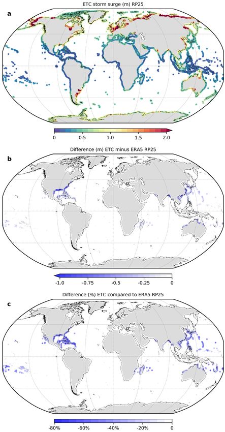
ARTICLE                                               COMMUNICATIONS EARTH & ENVIRONMENT | https://doi.org/10.1038/s43247-021-00204-9

Fig. 2 Extratropical cyclone-induced storm surge levels with a 25-year return period. The panels show the (a) 25-year extratropical cyclone storm surge
return period, (b) absolute difference (m) in surge levels between ERA5 and ETC, and (c) the relative difference (%) in surge levels between ERA5 and
ETC. The absolute and relative differences in surge level are calculated for the ETC-based RPs relative to ERA5, where ETC is similar to ERA5 but with the
tropical cyclones removed.

4            COMMUNICATIONS EARTH & ENVIRONMENT | (2021)2:135 | https://doi.org/10.1038/s43247-021-00204-9 | www.nature.com/commsenv
COMMUNICATIONS EARTH & ENVIRONMENT | https://doi.org/10.1038/s43247-021-00204-9                                                             ARTICLE

Fig. 3 Storm tide level return periods. The panels show the (a) 25-year storm tide return period, (b) crossover return period at which tropical cyclones
start to exceed extratropical cyclone storm tide levels, and Weibull’s plot showing tropical (blue) and extratropical cyclone (red) storm tide return periods,
together with the sum (black), at (c) New York, (d) The Hague, (e) Quanzhou, (f) Montevideo, (g) Toamasina, and (h) Cairns.

(1980–2017) of storm surge levels from a prior study26, which                   account (see “Methods” section). Subsequently, the RPs of TC-
forced GTSM with the ERA5 climate reanalysis. To prevent the                    induced and ETC-induced storm tides are computed separately
double-counting of TCs included in synthetic TC simulations, we                 and then probabilistically combined to determine the corre-
remove all TC-induced storm surges from the ERA5 surge levels                   sponding RPs. Storm tide levels exceeding 5.0 m are observed on
before calculating ETC storm surge RPs (see “Methods” section).                 all continents but with different forcing mechanisms. For exam-
The effect of removing TC storm surges from the ERA5 surge                      ple, in the Bay of Bengal and the Gulf of Mexico, TCs are the
levels on the RP25 surge level (Fig. 2b) is especially large in                 main drivers, while a large tidal range and ETC storm surges are
eastern China, north Australia, and the United States’ gulf and                 responsible for high storm tides in Europe and Canada. In north
east coasts with reductions of up to 1.0 m. This result is in line              Australia and the east coast of The United States, high storm tides
with the RP25 for TC storm surges, which shows the highest                      are typically caused by the coincidence of a TC or ETC with high
surge levels in the same regions. The relative effect (Fig. 2c) is              tide. In regions with both TCs and ETCs, ETCs influence most
large (>50%) in the previously named regions, as well as islands in             low RPs. RPs during which TC storm tide levels surpass those
the Caribbean, Pacific, and South Indian Oceans. These islands                   caused by ETCs (Fig. 3b) are low (
ARTICLE COMMUNICATIONS EARTH & ENVIRONMENT | https://doi.org/10.1038/s43247-021-00204-9
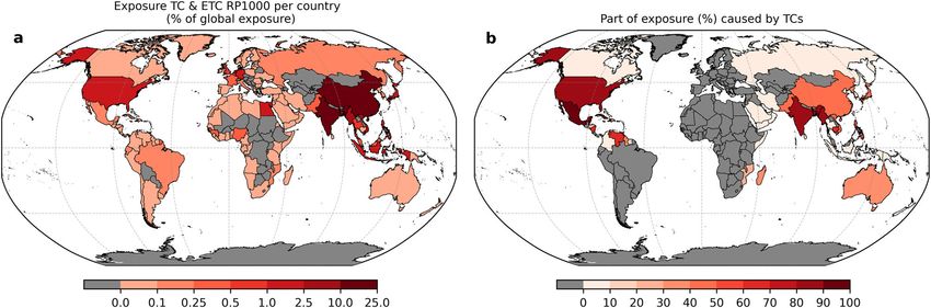
Fig. 4 Exposed population. The panels show the (a) number of people exposed to an RP1000 flood event per country relative to the global population,
taking TCs and ETCs into account, and (b) the part of the exposure caused by TCs per country. For countries depicted in gray on both subpanels, estimates
of exposure are equal to zero, while countries that are only gray on the right panel (b) are not affected by TCs that contribute to the country’s exposure.
than others, like the one in New York (United States). In New Table 1 Top ten countries exposed to RP1000 flood levels.
York, ETCs referred to as Nor’easters42, are the main source of
RP10 storm tides14,43. From RP45, storm tides are dominated by
Absolute Relative exposure
TCs, which can generate substantially higher storm tides com-
exposure (×1 (% of country
pared to ETCs at this location. The transition point, at which the million people) population)
influence of TCs and ETCs is equal in terms of the combined RP,
Country Total (% TC) Country Total (% TC)
shows the value of quality estimates of TC and ETC storm tide
Bangladesh 46.3 (91%) Netherlands 55.9 (0%)
RPs. It is interesting that along the northeast coast of the United India 37.0 (80%) Bahamas 43.2 (62%)
States the transition point is approximately RP100, as the 100- China 25.9 (49%) Bangladesh 28.4 (91%)
year flood zone is used by the National Flood Insurance Program Vietnam 13.6 (46%) Myanmar 15.7 (84%)
to determine who has to pay flood insurance and who can choose Netherlands 9.4 (0%) Vietnam 14.3 (45%)
to pay in the United States14,44. Finally, in Cairns (Australia), TC- Myanmar 8.8 (84%) Guyana 10.5 (38%)
induced storm tides surpass those caused by ETCs at RP391, Indonesia 4.6 (0%) Belgium 7.4 (0%)
showing how important it is to consider TCs when estimating United States 3.7 (86%) Greenland 6.4 (0%)
high RPs of storm tides, also if TCs are very rare compared to of America
ETCs36. Japan 3.5 (46%) Guinea 5.2 (0%)
To validate the COAST-RP dataset, we compare storm tide RPs Philippines 2.9 (55%) Albania 3.9 (0%)
with regional studies that use a similar approach along the World 191.6 (59%) World 2.5 (60%)
coastlines of Australia10,11 and the United States14,35. In general, The table shows the exposure to RP1000 flood levels for the top ten most exposed countries.
the comparison shows a good agreement. For the RP1000 storm Countries are ranked by estimates of absolute (left two columns) and relative exposure (right
two columns) to RP1000 flood levels. Here, relative exposure indicates the number of people
tide levels across 600 output locations in Australia, the root mean flooded per country relative to the country’s population. The number between brackets indicates
square error (RMSE), mean relative bias, and Spearman’s rank the contribution of TCs to the total exposure as a percentage.
coefficient are, respectively, 0.60 m, +2.9%, and 0.94. A possible
explanation for the positive bias is the higher resolution of GTSM
(2.5 km) compared to the grid used by ref. 10 (10 km). ref. 35 account (Fig. 4). This equals, respectively, 1.0% and 2.5% of the
presented storm tide RPs in the United States, only taking TCs global population (Table 1). The estimates of the exposed
into account. As COAST-RP indicates that the RP1000 for TC population are based on MERIT45 elevation data and the
storm tides surpass those induced by ETCs along the east coast of GPWv446 population for the year 2020. We assume no protection
the United States, the results can be compared. The RMSE, mean from coastal flooding because protection standards are below
relative bias and Spearman’s rank coefficient based on 23 output RP1000 along most global coastlines47. The exposure per country
locations are, respectively, 0.90 m, +5.8%, and 0.76. The relatively to TC and ETC RP1000 flood levels relative to the global exposure
small contribution of tides to storm tides along the United States (Fig. 4a) is especially large in Bangladesh (24%), India (19%),
coastline compared to Australia’s could explain the lower China (14%), and Vietnam (7%). This is a result of their large
Spearman’s rank coefficient. For all 23 output locations, our populations, as well as the high RP1000 storm tide levels
RP1000 storm tide levels fall within the 5th–95th percentiles as exceeding 3.0 m along most of the coastlines of these countries,
reported by ref. 35. Furthermore, one study14 assessed both TC even exceeding 10.0 m in the Bay of Bengal. Excluding the impact
and ETC storm tides for the New York area and estimated that of TCs (Supplementary Fig. 2), the relative exposure is largest in
TC storm tide levels surpass those of ETCs at a 60-year RP at The China (17%), followed by the Netherlands (12%), Vietnam (10%),
Battery, while we find a crossover RP of 45 years. Overall, the and India (9%). The relative contribution of TCs to total exposure
validation indicates good agreement of the COAST-RP dataset per country, relative to ETCs, is especially large (>90%) in Puerto
with regional studies. Rico, Belize, Cuba, Mexico, and Bangladesh (Fig. 4b); additionally
the United States and India are highly exposed to TC-induced
flooding. To explore which countries with small populations may
Flood exposure. Using a static flood model, we find that 77.8 be hit hard by an RP1000 flood event, we also calculate the
million people globally are exposed to the ETC RP1000 flood exposure per country relative to the country’s population
level. This increases to 191.6 million people when taking TCs into (Table 1). This way, countries with a small number of inhabitants
6 COMMUNICATIONS EARTH & ENVIRONMENT | (2021)2:135 | https://doi.org/10.1038/s43247-021-00204-9 | www.nature.com/commsenvCOMMUNICATIONS EARTH & ENVIRONMENT | https://doi.org/10.1038/s43247-021-00204-9 ARTICLE are also listed in the top 10 most exposed countries, such as the reducing away from the eye in a uniform way50–52 and that it Bahamas and Guyana (population 1000 km) from a TC in exposure analysis showed that 78 million people are exposed to regions like western Australia and Vietnam63,64. These waves are the ETC RP1000 flood level, which increased to 192 million not captured by GTSM as this would require a 3D hydrodynamic people when taking TCs into account. In addition, the exposure model. However, we believe the influence on our results is small estimate based on the COAST-RP RP1000 flood map is 31% as these waves generally do not exceed a few tens of centimeters higher compared to Aqueduct48, which is based on the GTSR and only become of interest when they coincide with the actual dataset18 and TC tracks from IBTrACS9. This indicates that storm surge. Last, GTSM is a 2D barotropic model and as such we previous studies have greatly underestimated the global exposure ignore mean sea level variability that is not driven by wind or by not fully accounting for low-probability TCs. atmospheric pressure65. Driven by steric changes and ocean cir- Several aspects of our methodology could be improved. First, culation, mean sea levels vary at seasonal to decadal timescales. the statistical resampling techniques underlying the STORM This effect can be up to 10 cm which adds to the occurrence of dataset do not account for physical characteristics28. The STORM extremes66. algorithm allows TCs to propagate within a 5° × 5° box based on The COAST-RP dataset provides an improved basis for large- the distribution of historical TC tracks in that box. For some scale flood risk assessments. By using synthetic TCs representing locations, this resolution is too coarse, and longer records of 3,000 years of data, this dataset represents a substantial observed TCs are required to better train the algorithm. As a improvement over existing global datasets, such as the Coastal result, in some areas there may be too many and too strong or too Dataset for the Evaluation of Climate Impact (CoDEC)26 and few and too weak TCs, resulting in an overestimation or under- others (e.g., refs. 18,19). Overall, we expect this to lead to higher estimation of TC-induced surge levels. For example, in the estimates of present-day flood risk in TC-prone regions, espe- northwest area of the Pacific, between 30° and 40° latitude, TCs cially in areas where the historical record includes too few or too tend to move toward the north or northeast9. However, TCs in weak TC events. In future research, we aim to apply the presented the STORM dataset also moved westward into the shallow and modeling framework to future scenarios and assess the impact of semi-enclosed Bohai Sea. As a result, modeled TC storm surges of climate change on storm tide RPs. While sea-level rise may be the up to 6.5 m largely exceeded the highest observed storm surges of dominant driver19, TCs and ETCs are projected to become more 2.5 m12,49. By applying a bias correction at output locations where intense in some areas. More specifically, most climate models the IBTrACS-based TC storm surge level RPs fall outside the indicate an increase in average TC intensity67 and project an 5th–95th percentiles of STORM (see “Methods” section), we average 5% increase in lifetime maximum surface wind speeds. In largely removed this bias. That said, it is inevitable that some addition, the number of slow-moving TCs is expected to overestimations or underestimations of storm tide RPs in TC- increase35,68, possibly resulting in prolonged coastal flooding. For prone regions remain in the COAST-RP dataset. ETCs, most climate models show a spatial shift of storm tracks, Second, we used the Holland parametric wind model to with a poleward shift in the Southern Hemisphere, for example, simulate wind and pressure fields for synthetic TCs. The Holland but do not indicate a clear change in ETC intensity69,70. When model assumes that a TC has a symmetric eye with wind speeds combining such information on future storminess with COMMUNICATIONS EARTH & ENVIRONMENT | (2021)2:135 | https://doi.org/10.1038/s43247-021-00204-9 | www.nature.com/commsenv 7
ARTICLE COMMUNICATIONS EARTH & ENVIRONMENT | https://doi.org/10.1038/s43247-021-00204-9
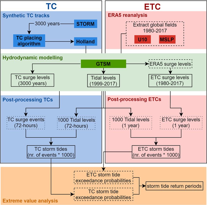
Fig. 5 Modeling framework. Flowchart showing the hydrodynamic modeling (green), and post-processing and extreme value analysis procedure (orange)
for each output location. ETC storm tide RPs are computed for each output location (red), and TC storm tide RPs are only included in TC-prone regions
(blue).
probabilistic projections of SLR along the coastline of the United period (19 years). Here, we used the same model setup as described in ref. 26, which
States, ref. 35 found that the historical RP100 will occur at least consisted of 23,226 output locations every 25 km along the global coastline. A
subset of 10,641 output locations located in regions prone to TCs was used for
every 30 years toward the end of the 21st century in the southeast simulating TC storm tides. The GTSM forced with ERA5 meteorological data has
Atlantic and the Gulf of Mexico. Such information on future- been validated in previous studies for both RPs of storm tides26 and individual TC
climate storm tide RPs is essential to accurately assess future flood events31.
risk and may prioritize adaptation efforts in areas facing the
highest flood risk.
TC storm surge modeling. To simulate TC-induced storm surges, we used a
dataset of synthetic TC tracks generated with the Synthetic Tropical cyclOne
Methods geneRation Model (STORM)28. The STORM dataset was created by statistically
General approach. Storm tides are driven by the combined effect of storm surges resampling climatological data from 38 years of best-track historical data found
and tides. To estimate the RPs of storm tides, we followed three main steps (Fig. 5). within the International Best Track Archive for Climate Stewardship (IBTrACS)9.
First, we separately simulated TC surge levels, ETC surge levels, and tidal levels. It was used to generate TCs representing 10,000 years of data under present-
Second, at each output location, we stochastically combined TC and ETC surge climate conditions. Variables extracted from STORM are U10, mean sea level
levels with random tidal levels to obtain TC and ETC storm tide levels, respectively. pressure (MSLP), longitude, latitude, and the radius to maximum winds (Rmax).
Third, we calculated the exceedance probabilities for TC and ETC storm tides using Hydrodynamic simulations conducted using GTSM are computationally expensive;
Weibull’s plotting position formula71 and probabilistically combined the two to therefore, we used different strategies to reduce the total runtime. First, from the
obtain storm tide RPs. 10,000 years of TC activity in STORM, we only simulated 3000 years of surge
levels, which is sufficient to reliably estimate the RP100076. Second, we only used
TC tracks that come within 750 km of land. Third, for each TC, we selected the part
Hydrodynamic model. Storm surges and tidal levels were simulated with the third of the track within 1000 km of the coast. Last, we simulated multiple TCs simul-
generation Global Tide and Surge Model (GTSMv3.0)26,72. The GTSMv3.0 is a taneously, resulting in another 70% reduction of the total runtime. To make that
global depth-averaged hydrodynamic model based on the Delft3D Flexible Mesh happen we used a newly developed algorithm that optimizes the spatiotemporal
software73. The resolution varies between 25 km in deeper parts of the ocean and placing of TCs77. To prevent a TC from being affected by any other TC, we set a
2.5 km along the coast (1.25 km for Europe). Storm surges can be simulated by minimum distance of 2000 km between TC tracks.
forcing GTSMv3.0 with wind and pressure fields. The stress exerted by the wind on For each TC track, wind speed, wind direction, and pressure fields were derived
the ocean was parameterized by multiplying the quadratic 10-m winds (U10) with using Holland’s parametric wind model50. The TC fields were represented by a
the atmospheric density and a user-defined wind drag coefficient (Cd), which polar grid with 36 radials, 375 arcs, and a 750 km radius. As the global median
depends on the surface roughness74,75. Tides were induced by including tide- values of the azimuthally-averaged radius of 12 ms−1 winds and outer radius of
generating forces using a set of 60 frequencies. The physical processes of internal historical TCs are 197 km and 423 km78, respectively, a 750 km radius will include
tides and self-attraction and loading were implemented in GTSMv3.072. To include all wind speeds capable of generating a significant storm surge79. As recommended
the 18.6-year nodal cycle, tidal levels were simulated with GTSM for the 1999–2017 by ref. 54, the counter-clockwise rotation angle was set at β = 20°, and the storm
8 COMMUNICATIONS EARTH & ENVIRONMENT | (2021)2:135 | https://doi.org/10.1038/s43247-021-00204-9 | www.nature.com/commsenvCOMMUNICATIONS EARTH & ENVIRONMENT | https://doi.org/10.1038/s43247-021-00204-9 ARTICLE
translation to surface background wind reduction factor was set at α = 0.55. An Second, all storm tide peaks exceeding the smallest tidal level of 19 yearly tidal
empirical surface wind reduction factor (SWRF) of 0.85 was used to adjust the maxima, which are at least 72-h apart to ensure independent events, were
wind fields at gradient levels to 10-m surface levels80. A wind conversion factor of extracted. We repeated this 1000 times to obtain the equivalent of 38,000 years of
0.915 was applied to convert winds from 1 min average to 10 min average81. The storm tide time series per output location. Last, we computed the empirical
inflow angle from ref. 82 was used to measure inward from the azimuthal direction, exceedance probabilities of ETC storm tides.
which increased linearly from 0° at the storm center to 10° at Rmax. Then, the Storm tide RPs were obtained per output location by taking the inverse of the
inflow angle increased further to 25° at 1.2 × Rmax and remained at 25° beyond. sum of the TC and ETC storm tide yearly exceedance frequency similar to ref. 14.
We used Garrat’s drag formula for 10-m wind speeds83 with Cd = (0.75 + For a given storm tide level x, we calculated its return period as follows:
0.067U10) × 10−3, which has been applied in numerous surge modeling 1
studies54,84. Cd is capped at Cd = 2.5 × 10⁻³ following ref. 85, as most studies agree RPðxÞ ¼ ð1Þ
that Cd begins to level off at wind speeds above 30 ms−1 86. The final product
1
RPTC ðxÞ þ RP 1
ETC ðxÞ
consisted of TC storm surge time series at a 10-min interval, representing 3000 where RP is the return period in years of storm tide level x. RPTC and RPETC refer
years of TC activity. to the return period of the TC and ETC storm tides at the same storm tide level,
Next, we applied a bias correction to the TC storm surge levels based on TC respectively. At output locations not affected by TCs, Eq. (1) simplifies to
storm surge levels for observed TCs. The reason for applying a bias correction is RP ¼ RPETC . Throughout the paper, variables like RP100 denote the 100-year RP.
that the synthetic TCs in STORM is too intense in some regions, resulting in storm This is because it is the storm tide level that is exceeded, on average, once every 100
tide RPs that are too high. The bias correction is based on three steps. First, we years, and has an exceedance probability of 0.01 (1/100) in any given year. The
simulated observed TC-induced storm surges by forcing GTSM with TC tracks EVA method presented here cannot assume storm surge levels exceeding the ones
from IBTrACS. Missing Rmax values in the IBTrACS dataset were computed based present in the input data92. This assumption could lead to an underestimation of
on the latitude and U10 of a TC, using estimates of TC geometry parameters per ETC storm tide RPs. To test whether this was the case, we compared our empirical
basin87. Second, we computed the 5th and 95th percentiles (i.e., 90% confidence approach with fitting extreme value distributions like Gumbel. The results did not
interval) for the STORM RPs based on bootstrapping using 599 repetitions. Per show an underestimation of ETC storm tide RPs (Supplementary Fig. 5;
output location, we computed the average storm surge level with an RP between 2 Supplementary Note 1). Therefore, we chose to apply the empirical EVA method.
and 19 years for IBTrACS and selected those output locations where the IBTrACS
value fell outside the 90% confidence interval of STORM (supplementary Fig. 3).
Last, at the selected locations, we multiplied all TC storm surge levels with a Modeling inundation and flood exposure. To demonstrate a first application of
correction factor (Supplementary Fig. 4) equal to the average 5th (when too low) or the COAST-RP dataset we computed flood exposure. We developed flood maps for
95th (when too high) percentile value divided by the average IBTrACS value. We the RP1000 storm tide level using a static inundation model that considers water
used this rather conservative linear scaling method, based on the 5th or 95th level attenuation48. The multi-error-removed improved-terrain digital elevation
percentile instead of the 50th percentile, because IBTrACS itself may underestimate model (MERIT DEM)45 at a 30-arcsecond resolution (approximately 1 km at the
or overestimate the exceedance probabilities due to its limited record length. In equator) was used as input. To account for surface roughness that reduces the
most regions where a bias correction has applied the magnitude of the bias water level inland93, a water level attenuation factor of 0.5 m km−1 was used. All
correction is negligible. The three main regions where a substantial correction areas with a direct connection to the sea and that have an elevation lower than the
factor is applied include the northeast coast of China (0.7), north Australia (1.4), water level that is reduced by the attenuation factor were inundated. Flood expo-
and the northern coastline of South America (0.6), with the average correction sure was measured in terms of the exposed population using the Gridded Popu-
factor in these regions indicated between brackets. Along the northeast coast of lation of the World version 4 (GPWv4)46 population count maps for the year 2020.
China the overestimation of TC storm surges can be explained by the fact that in They have been nationally adjusted to data from the United Nations World
STORM, TC intensification and weakening are modeled as a function of sea- Population Prospects 2015 Revision94. To test the sensitivity of the exposure
surface temperature28. As a result, a TC can continue to intensify in mid-latitude estimates to the population count maps, we also calculated the exposed population
regions as long as the sea surface temperature is high enough to sustain a TC, using WorldPop95 population count maps, which resulted in a 10% reduction of
whilst in reality, the TC will experience effects from enhanced wind shear and the TC and ETC exposure estimates. Flood protection was not included in the
extratropical transition. The underestimation in north Australia is caused by the analysis and would lead to an overestimation of the exposed population in areas
fact that this region is located near two TC basin boundaries of STORM. Since TCs protected against RP1000 flood events. That said, the flood extent could be
in STORM are cut off when they cross the basin boundary, this drives an underestimated in deltas and estuaries where the river may propagate the storm
underestimation of TC storm surges in the coastal region near Darwin. Last, the tide into the hinterland.
overestimation along the northern coastline of South America may be explained by
the additional error term that is applied by the STORM model to simulate a TC Data availability
track. This error term may cause the TC to move southward as opposed to the The COAST-RP dataset developed and applied during the study is available in the 4TU.
much more general north(westward) direction of observed TCs in these latitudinal
ResearchData data repository96 (https://doi.org/10.4121/13392314) and includes storm
regions.
tide levels with 1, 2, 5, 10, 25, 50, 100, 250, 500, and 1000-year RPs.
ETC storm surge modeling. To simulate ETC-induced storm surges, we made use
of wind and pressure fields from the ERA5 climate reanalysis88 from the European
Code availability
The TC placing algorithm and the Holland parametric wind model used to generate TC
Center for Medium-range Weather Forecasts (ECMWF). ERA5 has a horizontal
wind fields, written in Python, are available on github: https://github.com/nlesc-mosaic/
resolution of 0.25° × 0.25° and a temporal resolution of one hour. The ERA5-based
TCM (TC placing algorithm); https://github.com/NBloemendaal/STORM-return-periods
time series of storm surge levels were taken from Muis et al.26. We used the
(Holland parametric wind model). Other codes used to generate results reported in the
1980–2017 period for two reasons: (1) this period was used to generate the STORM
dataset. By using the same period, we ensured that the underlying climate condi- paper and central to its main claims are available upon request from the authors.
tions of the TC and ETC simulations were the same; and (2) to prevent the double
counting of TCs, we removed the TC-induced storm surges from the Received: 8 January 2021; Accepted: 10 June 2021;
ERA5 simulations using IBTrACS, which is complete from 1980 onwards when
reliable satellite observations became available. We assume that a storm surge is
induced by a TC when there is a TC within 250 km, until 48 h after the last
available time step of a TC track. TCs with a Rmax exceeding 50 km is likely to
affect a larger stretch of coastline. Therefore, we used a distance of 5 × Rmax if the
Rmax exceeds 50 km. A constant Charnock parameter was applied with a value of
0.04189 to translate wind speed into wind stress90. The final product consisted of 38 References
years of ETC storm surge time series at a 10-min interval. 1. Storch, H. & Woth, K. Storm surges: perspectives and options. Sustain. Sci. 3,
33–43 (2008).
2. Kulp, S. A. & Strauss, B. H. New elevation data triple estimates of global
Extreme value analysis. For TCs, we first detected all surge peaks that are at least vulnerability to sea-level rise and coastal flooding. Nat. Commun. 10, 1–12
three days apart to ensure independent events and we extracted surge levels from (2019).
24 h before until 48 h after the peak. Second, a 72-h tidal levels time series was 3. Koks, E. E. et al. A global multi-hazard risk analysis of road and railway
randomly sampled from the TC genesis month from any of the 19 available years infrastructure assets. Nat. Commun. 10, 1–11 (2019).
and combined with the extracted surge levels to obtain a 72-h storm tide levels time 4. Hinkel, J. et al. The ability of societies to adapt to twenty-first-century sea-level
series. Third, the highest storm tide level was extracted. This procedure was rise. Nat. Clim. Chang. 8, 570–578 (2018).
repeated 1000 times, resulting in 1000 maximum storm tide levels per surge peak. 5. Avila, L. A., Stewart, S. R., Berg, R. & Hagen, A. B. Tropical cyclone report:
Last, we computed the empirical exceedance probabilities of TC storm tides.
Hurricane Dorian. (National Hurricane Center, 2020).
For ETCs, a complete year of ETC surge levels, from January 1 until December
6. Beven, J. L., Berg, R. & Hagen, A. Tropical Cyclone Report: Hurricane Michael.
31, was combined with year-long tidal levels91. The tidal levels time series were
(National Hurricane Center, 2019).
randomly shifted between 30 days to include the full spring and neap tide cycle.
COMMUNICATIONS EARTH & ENVIRONMENT | (2021)2:135 | https://doi.org/10.1038/s43247-021-00204-9 | www.nature.com/commsenv 9ARTICLE COMMUNICATIONS EARTH & ENVIRONMENT | https://doi.org/10.1038/s43247-021-00204-9
7. Deutschländer, T., Friedrich, K., Haeseler, S. & Lefebvre, C. Severe storm 38. Lee, C. Y., Tippett, M. K., Sobel, A. H. & Camargo, S. J. An environmentally
XAVER across northern Europe from 5 to 7 December 2013. Deutscher forced tropical cyclone hazard model. J. Adv. Model. Earth Syst. 10, 223–241
Wetterdienst https://www.dwd.de/EN/ourservices/specialevents/storms/ (2018).
20131230_XAVER_europe_en.pdf?__blob=publicationFile&v=4 (2013). 39. Muis, S. et al. Spatiotemporal patterns of extreme sea levels along the western
8. Kendon, M. Storm Ciara. Met Office National Climate Information Centre North-Atlantic coasts. Sci. Rep. 9, 1–12 (2019).
https://www.meteo.be/nl/info/nieuwsoverzicht/storm-ciara (2020). 40. Rodwell, M. J. & Hoskins, B. J. Subtropical anticyclones and summer
9. Knapp, K. R., Kruk, M. C., Levinson, D. H., Diamond, H. J. & Neumann, C. J. monsoons. J. Clim. 14, 3192–3211 (2001).
The international best track archive for climate stewardship (IBTrACS): 41. Emanuel, K. A. & Rotunno, R. Polar lows as arctic hurricanes. Tellus A Dyn.
Unifying tropical cyclone best track data. Bull. Am. Meteorol. Soc. 91, 363–376 Meteorol. Oceanogr. 41, 1–17 (1989).
(2010). 42. Dolan, R. & Davis, R. Coastal storm hazards. J. Coast. Res. 103–114 (1994).
10. Haigh, I. D. et al. Estimating present day extreme water level exceedance 43. New York City Panel on Climate Change. Climate risk information 2013:
probabilities around the coastline of Australia: tides, extra-tropical storm Observations, climate change projections, and maps. (eds Rosenzweig, C. &
surges and mean sea level. Clim. Dyn. 42, 121–138 (2014). Solecki, W.) NPCC2. Prepared for use by the City of New York Special
11. Haigh, I. D. et al. Estimating present day extreme water level exceedance Initiative on Rebuilding and Resiliancy, (New York, NY, 2013).
probabilities around the coastline of Australia: tropical cyclone-induced storm 44. Rasmussen, D. J., Buchanan, M. K., Kopp, R. E. & Oppenheimer, M. A flood
surges. Clim. Dyn. 42, 139–157 (2014). damage allowance framework for coastal protection with deep uncertainty in
12. Zhang, H. & Sheng, J. Examination of extreme sea levels due to storm surges sea level rise. Earth’s Futur. 8, e2019EF001340 (2020).
and tides over the northwest Pacific Ocean. Cont. Shelf Res. 93, 81–97 (2015). 45. Yamazaki, D. et al. A high-accuracy map of global terrain elevations. Geophys.
13. Lin, N., Emanuel, K. A., Smith, J. A. & Vanmarcke, E. Risk assessment of Res. Lett. 44, 5844–5853 (2017).
hurricane storm surge for New York City. J. Geophys. Res. Atmos. 115, 1–11 46. CIESIN. Gridded population of the world, Version 4 (GWPv4): Population
(2010). count adjusted to match 2015 revision of UN WPP country totals, revision 11.
14. Orton, P. M. et al. A validated tropical-extratropical flood hazard assessment Palisades, NY: NASA Socioecnomic Data and Applications Center (SEDAC).
for New York Harbor. J. Geophys. Res. Ocean. 121, 8904–8929 (2016). https://doi.org/10.7927/H4PN93PB. (2018).
15. Wahl, T. et al. Understanding extreme sea levels for broad-scale coastal impact 47. Scussolini, P. et al. FLOPROS: an evolving global database of flood protection
and adaptation analysis. Nat. Commun. 8, 1–12 (2017). standards. Nat. Hazards Earth Syst. Sci. 16, 1049–1061 (2016).
16. Arns, A., Wahl, T., Haigh, I. D., Jensen, J. & Pattiaratchi, C. Estimating 48. Ward, P. J. et al. Aqueduct Floods Methodology. World Resources Institute:
extreme water level probabilities: a comparison of the direct methods and Technical Note www.wri.org/publication/aqueduct-floods-methodology
recommendations for best practise. Coast. Eng. 81, 51–66 (2013). (2020).
17. Aerts, J. C. J. H. et al. Evaluating flood resilience strategies for coastal 49. Feng, J., Li, D., Li, Y., Liu, Q. & Wang, A. Storm surge variation along the
megacities. Science 344, 473–475 (2014). coast of the Bohai Sea. Sci. Rep. 8, 1–10 (2018).
18. Muis, S., Verlaan, M., Winsemius, H. C., Aerts, J. C. J. H. & Ward, P. J. A 50. Holland, G. J. An analytic model of the wind and pressure profiles in
global reanalysis of storm surges and extreme sea levels. Nat. Commun. 7, hurricanes. Mon. Weather Rev. 108, 1212–1218 (1980).
1–12 (2016). 51. Holland, G. J., Belanger, J. I. & Fritz, A. A revised model for radial profiles of
19. Vousdoukas, M. I. et al. Global probabilistic projections of extreme sea levels hurricane winds. Mon. Weather Rev. 138, 4393–4401 (2010).
show intensification of coastal flood hazard. Nat. Commun. 9, 2360 (2018). 52. Musinguzi, A., Akbar, M. K., Fleming, J. G. & Hargrove, S. K. Understanding
20. Vafeidis, A. T. et al. A new global coastal database for impact and vulnerability hurricane storm surge generation and propagation using a forecasting model,
analysis to sea-level rise. J. Coast. Res. 24, 917–924 (2008). forecast advisories and best track in a wind model, and observed data—case
21. Schuerch, M. et al. Future response of global coastal wetlands to sea-level rise. study hurricane Rita. J. Mar. Sci. Eng. 7, 77 (2019).
Nature 561, 231–234 (2018). 53. Knaff, J. A., Kossin, J. P. & DeMaria, M. Annular hurricanes. Weather Forecast
22. Jongman, B., Ward, P. J. & Aerts, J. C. J. H. Global exposure to river and 18, 204–223 (2003).
coastal flooding: Long term trends and changes. Glob. Environ. Chang 22, 54. Lin, N. & Chavas, D. On hurricane parametric wind and applications in storm
823–835 (2012). surge modeling. J. Geophys. Res. 117, 19 (2012).
23. Hinkel, J. et al. Coastal flood damage and adaptation costs under 21st century 55. Emanuel, K. & Rotunno, R. Self-stratification of tropical cyclone outflow. Part
sea-level rise. Proc. Natl Acad. Sci. USA 111, 3292–3297 (2014). I: implications for storm structure. J. Atmos. Sci. 68, 2236–2249 (2011).
24. Hinkel, J. & Klein, R. J. T. Integrating knowledge to assess coastal vulnerability 56. Hu, K., Chen, Q. & Kimball, S. K. Consistency in hurricane surface wind
to sea-level rise: the development of the DIVA tool. Glob. Environ. Chang 19, forecasting: an improved parametric model. Nat. Hazards 61, 1029–1050
384–395 (2009). (2012).
25. Tiggeloven, T. et al. Global-scale benefit-cost analysis of coastal flood 57. Chavas, D. R., Lin, N. & Emanuel, K. A model for the complete radial
adaptation to different flood risk drivers using structural measures. Nat. structure of the tropical cyclone wind field. Part I: Comparison with observed
Hazards Earth Syst. Sci. 20, 1025–1044 (2020). structure. J. Atmos. Sci. 72, 3647–3662 (2015).
26. Muis, S. et al. A high-resolution global dataset of extreme sea levels, tides, and 58. Horsburgh, K. J. & Wilson, C. Tide-surge interaction and its role in the
storm surges, including future projections. Front. Mar. Sci. 7, 263 (2020). distribution of surge residuals in the North Sea. J. Geophys. Res. Ocean. 112,
27. Vitousek, S. et al. Doubling of coastal flooding frequency within decades due C08003 (2007).
to sea-level rise. Sci. Rep. 7, 1–9 (2017). 59. Santamaria-Aguilar, S. & Vafeidis, A. T. Are extreme skew surges independent
28. Bloemendaal, N. et al. Generation of a global synthetic tropical cyclone hazard of high water levels in a mixed semidiurnal tidal regime? J. Geophys. Res.
dataset using STORM. Sci. Data 7, 1–12 (2020). Ocean. 123, 8877–8886 (2018).
29. Weinkle, J., Maue, R. & Pielke, R. Historical global tropical cyclone landfalls. J. 60. Arns, A. et al. Non-linear interaction modulates global extreme sea levels,
Clim. 25, 4729–4735 (2012). coastal flood exposure, and impacts. Nat. Commun. 11, 1–9 (2020).
30. Pugh, D. T. & Woodworth, P. L. Sea-Level Science: Uderstanding Tides, Surges, 61. Stewart, R. H. Introduction to Physical Oceanography. (Department of
Tsunamis And Mean Sea-level Changes. (Cambridge University Press, Oceanography, Texas A and M University, 2008). https://doi.org/10.1119/
Cambridge, New York, 2014). 1.18716.
31. Dullaart, J. C. M., Muis, S., Bloemendaal, N. & Aerts, J. C. J. H. Advancing 62. Kirezci, E. et al. Projections of global-scale extreme sea levels and
global storm surge modelling using the new ERA5 climate reanalysis. Clim. resulting episodic coastal flooding over the 21st century. Sci. Rep. 10, 1–12
Dyn. 54, 1007–1021 (2020). (2020).
32. Vickery, P. J., Skerlj, P. F. & Twisdale, L. A. Simulation of hurricane risk in the 63. Trinh, T. T., Pattiaratchi, C. & Bui, T. The contribution of Forerunner to
U.S. using empirical track model. J. Struct. Eng. 126, 1222–1237 (2000). storm surges along the Vietnam Coast. J. Mar. Sci. Eng. 8, 508 (2020).
33. Hardy, T. A., McConochie, J. D. & Mason, L. B. Modeling tropical cyclone 64. Eliot, M. & Pattiaratchi, C. Remote forcing of water levels by tropical cyclones
wave population of the Great Barrier Reef. J. Waterw. Port Coast. Ocean Eng. in Southwest Australia. Cont. Shelf Res. 30, 1549–1561 (2010).
129, 104–113 (2003). 65. Muis, S., Haigh, I. D., Guimarães Nobre, G., Aerts, J. C. J. H. & Ward, P. J.
34. James, M. K. & Mason, L. B. Synthetic tropical cyclone database. J. Waterw. Influence of El Niño-Southern Oscillation on Global Coastal Flooding. Earth’s
Port Coast. Ocean Eng. 131, 181–192 (2005). Futur. 6, 1311–1322 (2018).
35. Marsooli, R., Lin, N., Emanuel, K. & Feng, K. Climate change exacerbates 66. Rashid, M. M., Wahl, T., Chambers, D. P., Calafat, F. M. & Sweet, W. V. An
hurricane flood hazards along US Atlantic and Gulf Coasts in spatially varying extreme sea level indicator for the contiguous United States coastline. Sci.
patterns. Nat. Commun. 10, 1–9 (2019). Data 6, 1–14 (2019).
36. Lin, N. & Emanuel, K. Grey swan tropical cyclones. Nat. Clim. Chang. 6, 67. Knutson, T. et al. Tropical cyclones and climate change assessment. Part II:
106–111 (2016). Projected response to anthropogenic warming. Bull. Am. Meteorol. Soc. 101,
37. Emanuel, K., Ravela, S., Vivant, E. & Risi, C. A statistical deterministic 303–322 (2020).
approach to hurricane risk assessment. Bull. Am. Meteorol. Soc. 87, 299–314 68. Kossin, J. P. A global slowdown of tropical-cyclone translation speed. Nature
(2006). 558, 104–107 (2018).
10 COMMUNICATIONS EARTH & ENVIRONMENT | (2021)2:135 | https://doi.org/10.1038/s43247-021-00204-9 | www.nature.com/commsenvCOMMUNICATIONS EARTH & ENVIRONMENT | https://doi.org/10.1038/s43247-021-00204-9 ARTICLE
69. Baatsen, M., Haarsma, R. J., Van Delden, A. J. & de Vries, H. Severe autumn 94. U. N. United Nations, Department of Economic and Social Affairs, Population
storms in future western Europe with a warmer Atlantic Ocean. Clim. Dyn. 45, Divison. World Population Prospects: The 2015 Revision. https://population.
949–964 (2015). un.org/wpp/ (2015).
70. Michaelis, A. C., Willison, J., Lackmann, G. M. & Robinson, W. A. Changes in 95. Tatem, A. J. WorldPop, open data for spatial demography. Sci. Data 4, 1–4
winter North Atlantic extratropical cyclones in high-resolution regional (2017).
pseudo-global warming simulations. J. Clim. 30, 6905–6925 (2017). 96. Dullaart, J. C. M. et al. COAST-RP: A global COastal dAtaset of Storm
71. Coles, S. An Introduction to Statistical Modeling of Extreme Values. Springer Tide Return Periods. 4TU.ResearchData. https://doi.org/10.4121/13392314.
Series in Statistics (Springer London, 2001). (2021).
72. Irazoqui Apecechea, M., Verlaan, M., Zijl, F., Le Coz, C. & Kernkamp, H.
Effects of self-attraction and loading at a regional scale: a test case for the
Northwest European shelf. Ocean Dyn. 67, 729–749 (2017). Acknowledgements
73. Kernkamp, H. W. J., Van Dam, A., Stelling, G. S. & de Goede, E. D. Efficient We would like to thank Martin Verlaan and Maialen Irazoqui Apecechea from
scheme for the shallow water equations on unstructured grids with application Deltares for their support with the use of GTSM. The authors also acknowledge
to the Continental Shelf. Ocean Dyn. 61, 1175–1188 (2011). Arne Arns for sharing his thoughts on the statistical analysis. We would also like to
74. Pugh, D. T. Tides, Surges and Mean Sea-level (Reprinted with corrections). thank Ivan Haigh and Reza Marsooli for providing validation data. We thank Maxime
(John Wiley & Sons, Ltd., 1996). Moge from SURFsara (http://www.surfsara.nl) for his support in using the Cartesius
75. Zweers, N. C., Makin, V. K., de Vries, J. W. & Burgers, G. On the influence of Computer Cluster. J.D. received funding from the COASTRISK project financed by the
changes in the drag relation on surface wind speeds and storm surge forecasts. SCOR Corporate Foundation for Science (R/003316.01). S.M. and M.C. received funding
Nat. Hazards 62, 207–219 (2012). from the research program MOSAIC with project number ASDI.2018.036, which is
76. Hardy, T., Mason, L. & Astorquia, A. Queensland Climate Change and financed by the NWO. N.B. and J.A. are funded by a VICI grant from the Netherlands
Community Vulnerability to Tropical Cyclones-Ocean Hazards Assessment- Organization for Scientific Research (NWO) (Grant Number 453-13-006) and the
Stage 3: the Frequency of Surge plus Tide during Tropical Cyclones for Selected ERC Advanced Grant COASTMOVE #884442. A.C. was supported by the Dutch
Open Coast Locations along the Queensland East Coast. https://doi.org/ Research Council (NWO) (VIDI; grant no. 016.161.324). This work was sponsored by
10.13140/RG.2.1.4856.5928. (2004). NWO Exact and Natural Sciences for the use of supercomputer facilities (grant no.
77. Chertova, M., Muis, S., Pelupessy, I. & Ward, P. Incorporating large datasets 2020.007).
of synthetic tropical cyclones with Global Tide and Surge Model (GTSM) for
global assessment of extreme sea levels. In 22nd EGU General Assembly Author contributions
EGU2020-21189, https://doi.org/10.5194/egusphere-egu2020-21189 (2020). J.D. performed the hydrodynamic modeling and analysis and wrote the paper. S.M.
78. Chavas, D. R. & Emanuel, K. A. A QuikSCAT climatology of tropical cyclone carried out the inundation modeling, M.C. developed the tropical cyclone placing
size. Geophys. Res. Lett. 37, L18816 (2010). algorithm, and A.C. assisted in the statistical analysis. N.B. and J.A. participated in
79. Kalourazi, M. Y., Siadatmousavi, S. M., Yeganeh-Bakhtiary, A. & Jose, F. technical discussions and all authors co-wrote the paper.
Simulating tropical storms in the Gulf of Mexico using analytical models.
Oceanologia 62, 173–189 (2019).
80. Batts, M. E., Cordes, M. R., Russel, L. R., Shaver, J. R. & Simiu, E. Hurricane Competing interests
wind speeds in the United States. NBS Build. Sci. Ser. 124, 50 (1980). The authors declare no competing interests.
81. Harper, B. A., Kepert, J. D. & Ginger, J. D. Guidelines for Converting between
Various Wind Averaging in Tropical Cyclone Conditions. https://library.wmo.
int/doc_num.php?explnum_id=290 (2010).
Additional information
Supplementary information The online version contains supplementary material
82. Queensland Government. Queensland Climate Change and Community
available at https://doi.org/10.1038/s43247-021-00204-9.
Vulnerability to Tropical Cyclones: Ocean Hazards Assessment-stage 1. http://
www.systemsengineeringaustralia.com.au/download/Ocean_Hazards_Assess_
Correspondence and requests for materials should be addressed to J.C.M.D.
Stage1A_revised.pdf (2001).
83. Garratt, J. R. Review of drag coefficients over oceans and continents. Mon. Peer review information Communications Earth & Environment thanks the anonymous
Weather Rev. 105, 915–929 (1977). reviewers for their contribution to the peer review of this work. Primary Handling
84. Westerink, J. J. et al. A basin- to channel-scale unstructured grid hurricane Editors: Adam Switzer and Joe Aslin. Peer reviewer reports are available.
storm surge model applied to southern Louisiana. Mon. Weather Rev. 136,
833–864 (2008). Reprints and permission information is available at http://www.nature.com/reprints
85. Powell, M. D., Vickery, P. J. & Reinhold, T. A. Reduced drag coefficient for
high wind speeds in tropical cyclones. Nature 422, 279–283 (2003).
Publisher’s note Springer Nature remains neutral with regard to jurisdictional claims in
86. Sterl, A. Drag at high wind velocities-a review, Technical Report. TR-361.
published maps and institutional affiliations.
http://projects.knmi.nl/publications/fulltexts/sterl_review_drag_tr361_2017.
pdf (2017).
87. Nederhoff, K., Giardino, A., Van Ormondt, M. & Vatvani, D. Estimates of
tropical cyclone geometry parameters based on best-track data. Nat. Hazards Open Access This article is licensed under a Creative Commons
Earth Syst. Sci. 19, 2359–2370 (2019). Attribution 4.0 International License, which permits use, sharing,
88. Hersbach, H. et al. Global reanalysis: goodbye ERA-Inteirm, hello ERA5. adaptation, distribution and reproduction in any medium or format, as long as you give
ECMWF Newsl 159, 17–24 (2019). appropriate credit to the original author(s) and the source, provide a link to the Creative
89. Charnock, H. Wind stress on a water surface. Q. J. R. Meteorol. Soc. 81, Commons license, and indicate if changes were made. The images or other third party
639–640 (1955). material in this article are included in the article’s Creative Commons license, unless
90. Bryant, K. M. & Akbar, M. An exploration of wind stress calculation indicated otherwise in a credit line to the material. If material is not included in the
techniques in hurricane storm surge modeling. J. Mar. Sci. Eng. 4, 58 (2016). article’s Creative Commons license and your intended use is not permitted by statutory
91. Goring, D. G., Stephens, S. A., Bell, R. G. & Pearson, C. P. Estimation of regulation or exceeds the permitted use, you will need to obtain permission directly from
extreme sea levels in a tide-dominated environment using short data records. the copyright holder. To view a copy of this license, visit http://creativecommons.org/
J. Waterw. Port Coast. Ocean Eng. 137, 150–159 (2011). licenses/by/4.0/.
92. Fortunato, A. B., Li, K., Bertin, X., Rodrigues, M. & Miguez, B. M.
Determination of extreme sea levels along the Iberian Atlantic coast. Ocean
Eng. 111, 471–482 (2016). © The Author(s) 2021
93. Vafeidis, A. T. et al. Water-level attenuation in broad-scale assessments of
exposure to coastal flooding: a sensitivity analysis. Nat. Hazards Earth Syst.
Sci. 19, 973–984 (2019).
COMMUNICATIONS EARTH & ENVIRONMENT | (2021)2:135 | https://doi.org/10.1038/s43247-021-00204-9 | www.nature.com/commsenv 11You can also read