Accurate diagnosis of prostate cancer using logistic regression
←
→
Page content transcription
If your browser does not render page correctly, please read the page content below
Open Medicine 2021; 16: 459–463
Research Article
Arash Hooshmand*
Accurate diagnosis of prostate cancer using
logistic regression
https://doi.org/10.1515/med-2021-0238 throughput Omics technologies, we are no longer missing
received September 2, 2020; accepted January 29, 2021 data but need novel methods and techniques to handle
Abstract: A new logistic regression-based method to and analyze them; thus, bioinformatics and computers
distinguish between cancerous and noncancerous RNA have found a solid ground to contribute in life sciences.
genomic data is developed and tested with 100% preci- One of the most applicable approaches to benefit from
sion on 595 healthy and cancerous prostate samples. A computer science in physiology and medicine is utiliza-
logistic regression system is developed and trained using tion of artificial intelligence to extract knowledge by com-
whole-exome sequencing data at a high-level, i.e., nor- puters out of big data generated by Omics technologies [4].
malized quantification of RNAs obtained from 495 pros- In this work, we have developed a logistic regression
tate cancer samples from The Cancer Genome Atlas and (LGR) system using general new generation of RNA
100 healthy samples from the Genotype-Tissue Expres- Seq. data that can detect any prostate cancer, and hence
sion project. We could show that both sensitivity and will decrease the risk of mortality by correct diagnosis.
specificity of the method in the classification of cancerous The Omics technologies and their corresponding big data
and noncancerous cells are perfectly 100%. analysis tools are developing fast and getting cheaper
and more widespread all the time. Currently, the third
Keywords: machine learning, prostate cancer, diagnosis, generation of sequencing methods such as quantum
transcriptome, RNA sequencing, high throughput technol- sequencing [5], nanopore sequencing [6], and single-
ogies, logistic regression, classification molecule real-time sequencing [7] are making it possible
even today for the wealthy people to benefit from expen-
sive analyses, and if the current trend in advancements
continues, it will not be a long way left to have common-
1 Introduction place analytical tools and services in each hospital and
city. The advantage of machine learning is that as it gets
Prostate cancer is one of the severe cancers in men. more and more samples, its training would be more
According to the US cancer statistics report for 2020, matured and more robust; therefore, there is a hope that
there are estimated 191,930 new cases of prostate cancer the 100% accuracy that is achieved by a modest amount
and 33,330 deaths because of it, and the importance of of data can be stabilized in the future when many
early diagnosis has repeatedly been emphasized [1]. Bio- patients and healthy people samples are fed to the
logists have discovered many genes that are involved in system.
specific cancers; for example, BRCA1 in breast cancer [2] Computational techniques and tools are rapidly
and STAT3 in prostate cancer [3]. In diagnosis and cancer opening their positions in medical and pharmaceutical
identification, histological examination is used as gold sciences too [8]. Different methods have been developed
standard but it is a slow process and needs technical and tested in the last few decades and have returned
experts and suffers from large amount of variations great results in different fields of medicine including
among observers. In recent years, thanks to high but not limited to cancer identification [9]. In this work,
we have come up with a novel approach of applying LGR
for cancer detection that is effective and robust. Using our
method, cancerous tissue can correctly be identified, thus
* Corresponding author: Arash Hooshmand, Department of
providing an opportunity to be controlled on time. This
Biomedical Engineering and Health Systems, School of Engineering
Sciences in Chemistry, Biotechnology and Health, KTH Royal
approach also offers a new direction for disease diagnosis
Institute of Technology, 11428 Stockholm, Sweden, while providing a new method to predict traits based on
e-mail: hooshmand@kth.se genomic information.
Open Access. © 2021 Arash Hooshmand, published by De Gruyter. This work is licensed under the Creative Commons Attribution 4.0
International License.460 Arash Hooshmand
2 Methods 2.2 Feature selection
In this project, we have used LGR algorithm from Sci- There are wrong perceptions in the computer science
Kit Learn on 495 samples from The Cancer Genome community about life science data that have prevented
Atlas (TCGA) research network and 100 samples of the potential achievements, for instance, one is about the
Genotype-Tissue Expression (GTEx) project portal and number of features [11] such as “it is obviously imprac-
directly fed the genome data to the machine to do heavy tical to select all of the genes because mass dimensions
statistical calculations on our high dimensional data. The will increase the computation cost.” As a result,
different parts of the method are clarified below. We use researchers usually try to reduce the assumed computa-
all the available data at the time of accessing the data- tional costs allegedly brought about by highly redundant
bases and have not ignored any sample. dimensions and select a subset of features, i.e., genes to
reduce the number of features and dimensions [12]. A
strength point of our work is that we gave all the data
corresponding to the whole-exome sequencing as feature
2.1 Binary LGR inputs to the logistic regressor at once and it returned
almost perfect results quickly and precisely. We thought
The LGR is a group of statistical techniques that aim to of 19,627 different genes not as too many features but as
test hypotheses or causal relationships when the depen- different pixels of a less than 141 × 141 pixel photo, in
dent variable is nominal. which there are correlated pixels too, and it was a very
Despite its name, it is not an algorithm applied in light task for the machine to analyze such a low-resolu-
regression problems, in which continuous values are tion image and it took only seconds to classify the can-
dealt with, but it is a method for classification problems, cerous and noncancerous cells 100% precisely.
in which a binary value, i.e., either 0 or 1 is obtained. For
example, a classification problem is to identify if a given
tumor is malignant or benign. With the LGR, the relation-
ship between the dependent variable, i.e., the statement 2.3 Model settings and evaluation
to be predicted, with one or more independent variables,
i.e., the set of features available for the model is deter- We have used LGR classifier also known as Logit or
mined. To do this, it uses a logistic function that deter- MaxEnt classifier from Scikit-Learn 0.23.1 with its default
mines the probability of the dependent variable. As settings. Model evaluation produces measures to approx-
previously mentioned, what is sought in these problems imate a classifier’s reliability. To distinguish between
is a classification, so the probability must be translated cancerous and noncancerous cells, as it is a binary clas-
into binary values for which a threshold value is used. sification, we use accuracy, precision, specificity, sensi-
If the probability values were above the threshold tivity, f1 score, several averaging techniques, and receiver
value, the statement is true and vice versa. Generally, operating characteristic curve to evaluate the model. We,
this value is 0.5, although it can be increased or indeed, use Sci-kit Learn Metrics Classification Report
decreased to manage the number of false positives or that returns precision, recall, and f1 score for each of
false negatives [10]. two classes. In binary classification, recall of the positive
In supervised classification methods the input data, class is called “sensitivity,” and recall of the negative
usually seen as p points, are viewed as a p-dimensional class is “specificity.” In what follows, the terms and deri-
vector (an array or ordered list of p numbers). Then the vations from confusion matrix such as accuracy, specifi-
classifiers are more or less based on similar criteria, e.g., city, sensitivity, and f1 score are given to review and
in the Bayesian classifiers, the classifier looks for a hyper compare:
surface that maximizes the likelihood of drawing the Condition positive (P): the number of real positive cases
sample, or in SVMs, it looks for a hyperplane that opti- in the data
mally separates the points of one class from the other, Condition negative (N): the number of real negative
which eventually could have been previously projected to cases in the data
a higher dimensional space. The LGR is a generalization True positive (TP) or hit
of logits to distinguish samples that belong to one of the True negative (TN) or correct rejection
two different classes; hence, it is usually called binary False positive (FP), false alarm, or type I error
LGR. False negative (FN), miss, or type II errorCancer diagnosis by logistic regression 461
Sensitivity, recall, hit rate, or true-positive rate (TPR): As we are using Sci-kit Learn Metrics Classification
TPR = TP / P = TP /(TP + FN) = 1 − FNR. (1) Report to show the results as shown in Table 1, we also
describe the meaning of micro avg, macro avg, and
Specificity, selectivity, or true-negative rate (TNR): weighted avg. used in the report: Micro-average of preci-
TNR = TN / N = TN /(TN + FP) = 1 − FPR. (2) sion (MIAP):
Precision or positive predictive value (PPV) is the MIAP = (TP1 + TP2)/(TP1 + TP2 + FP1 + FP2). (11)
ratio of the correctly labeled samples by our program to Micro-average of recall (MIAR):
all labeled ones in reality.
MIAR = (TP1 + TP2)/(TP1 + TP2 + FN1 + FN2). (12)
PPV = TP /(TP + FP) = 1 − FDR. (3)
Micro-average of f-score (MIAF) would be the har-
Precision can be calculated only for the positive monic mean of the two numbers above.
class, i.e., class 1 that shows cancer or can be evaluated
MIAF = 2· MIAP· MIAR/(MIAP + MIAR). (13)
for each one of the two classes independently treating
each class as it is the positive class at time, and the latter Macro-average of precision (MAAP):
is done in Sci-kit Learn Metrics Classification Report as MAAP = (Precision 1 + Precision 2)/ 2. (14)
shown in Table 1.
Negative predictive value (NPV): Macro-average of recall (MAAR):
NPV = TN /(TN + FN) = 1 − FOR. (4) MAAR = (Recall 1 + Recall 2)/ 2. (15)
Miss rate or false-negative rate (FNR): Macro-average of f-score (MAAF) would be the har-
monic mean of the two numbers above.
FNR = FN / P = FN /(FN + TP) = 1 − TPR. (5)
MAAF = 2· MAAP · MAAR /(MAAP + MAAR). (16)
Fall-out or false-positive rate (FPR):
Macro-average method is suitable to know how the
FPR = FP / N = FP /(FP + TN) = 1 − TNR. (6)
system performs overall across different sets of data
False discovery rate (FDR): but should not be considered in any specific decision-
FDR = FP /(FP + TP) = 1 − PPV. (7) making because it calculates metrics for each label and
finds their unweighted mean, i.e., it does not take label
False omission rate (FOR): imbalance into account, while in our case, the labels are
FOR = FN /(FN + TN) = 1 − NPV. (8) highly imbalanced, i.e., 495 vs 100. On the contrary,
micro-average is a useful tool and returns measures for
Accuracy (ACC): decision-making especially when datasets vary in size
ACC = (TP + TN)/( T + N) because it calculates metrics globally by counting the
(9) total true-positives, false-negatives, and false-positives.
= (TP + TN)/(TP + TN + FP + FN).
Finally, weighted-average, according to Sci-kit Learn
The harmonic mean of precision and sensitivity or f1 documentation on f1-score metrics, calculates metrics
score (F1): for each label and finds their average weighted by sup-
port (the number of true instances for each label). This
F1 = 2·PPV · TPR/(PPV + TPR)
(10) alters “macro” to account for label imbalance; conse-
= 2·TP /(2·TP + FP + FN). quently, it can result in an F-score that is not between
precision and recall.
Table 1: Classification report
3 Results
Summary Precision Recall f1 score Support
Class 0 1.00 1.00 1.00 9 Genomic variation files of 595 samples including healthy
Class 1 1.00 1.00 1.00 51 people (100 individuals) and cancer patients (495 indivi-
Micro avg. 1.00 1.00 1.00 60 duals) were obtained from the GTEx Project and the TCGA
Macro avg. 1.00 1.00 1.00 60
online database. The binary classification results of can-
Weighted avg. 1.00 1.00 1.00 60
cerous and noncancerous samples were great because462 Arash Hooshmand
difference between two classes is so much that providing
hundreds of samples enables the machine to distinguish
between two categories containing 495 and 100 samples
perfectly. It is also useful to consider the fact that TCGA
and GTEx data are not perfect and there are several rows
of missing data for some of gene quantities in some sam-
ples, yet the data provided by these two projects are fairly
clean and reliable and it was enough for our classifier to
be able to do its classification 100% correctly. This system
is trained now to receive any new person’s RNA-seq data
and recognize if the patient’s prostate is cancerous or not.
The limitation of our model is that it needs future colla-
boration with both hospitals and well-equipped labora-
tories and also needs the whole genome data of samples
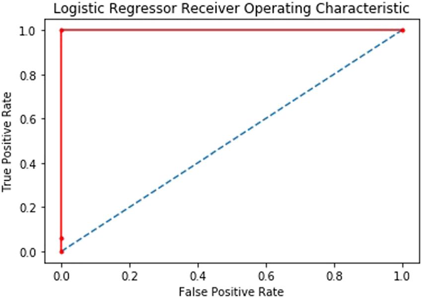
Figure 1: ROC curve of LGR classifier performance in distinguishing
from the organ, and the involving labs should follow the
cancerous and noncancerous prostate cells.
same protocols to obtain the transcriptomics data.
Therefore, we cannot add training data from other
the system can detect all cancerous and noncancerous sources and databases to include as many samples as
samples correctly and as seen in the classification report we want. Fortunately, we do not need to do it because
shown in Table 1, the performance of the classifier is our data have been enough to train the system and
perfect with accuracy and precision of 100% and sensi- achieve perfect classification ability. Furthermore, an
tivity and specificity of 1. In this classification, not only advantage of our approach is that we have used a classic
the accuracy is 100% but also the receiver operating char- interpretable method that is based on statistics, unlike
acteristic’s area under curve (ROC AUC) from prediction other works such as Sun et al. [13] who have used com-
scores also would be 1 as seen in Figure 1. plex neural networks that act as a black box and are not
interpretable. Nevertheless, obtaining the whole-exome
sequencing data of 19,627 genes as done by GTEx and
TCGA on samples obtained from people’s prostates is at
4 Discussion research level and is not yet a cheap procedure or
common practice for general hospitals. However, the
The classifier did its task perfectly with no error, at least New Generation RNA-seq protocols followed by GTEx
on our available data. There are yet some aspects to and TCGA are well known and standard, and as technol-
reflect on. Although most TCGA prostate cancer (PRAD) ogies are developed rapidly, they are continuously get-
comprise white men’s samples, they have considered ting cheaper and more practical than before. Meanwhile,
human variations to contain samples of different races the next topic of research can be finding suitable biomar-
and groups as well to represent the US demographic kers in the blood that can detect healthy people and
information fairly. As our method classifies all can- patients only by their blood tests.
cerous and non-cancer samples correctly using the
information available in genomic variation, it can Acknowledgments: The author thanks Houshmand family
mean that the genetic signatures of cancer are detected and their companies, especially Mr. Eng. GholamAbbas
universally without the need to consider racial or sexual Houshmand, then Atash Houshmand, Shahab Houshmand,
differences. Shahin Houshmand, and Shadab Houshmand who financed
Our work provided a new approach in application of all the study and research during several years. The
computers using medical data that resulted in excellent author also thanks the library of KTH Royal Institute of
classification between cancerous and noncancerous cells Technology for financial support of the publication fee.
of the prostate. In this work, we did not reduce the
dimension of input data and left all the statistical ana- Ethical approval: This project does not need any extra
lysis to the computer, and it could do its job very well and personal/patient consent approval either because the
distinguished the cancerous samples from healthy cells data are normalized and do not reveal any private infor-
almost perfectly. We even did not need to balance the mation, and whatever necessary with respect to the law is
number of samples of each class and it shows that the observed by the institutes publishing them.Cancer diagnosis by logistic regression 463
Conflict of interest: The author is the only author of this [4] Nik-Zainal S, Memari Y, Davies HR. Holistic cancer genome
article who has submitted it to De Gruyter’s Open profiling for every patient. Swiss Med Wkly. 2020;150:w20158.
Medicine journal, and hence reiterates the consent to [5] Di Ventra M, Taniguchi M. Decoding DNA, RNA and
peptides with quantum tunnelling. Nat Nanotechnol.
publish it in this journal. There are no competing inter-
2016;11(2):117–26.
ests and there is no need for any other consent approvals. [6] Branton D, Deamer DW, Marziali A, Bayley H, Benner SA,
Butler T, et al. The potential and challenges of nanopore
Data availability statement: The datasets generated dur- sequencing. Nat Biotechnol. 2008;26(10):1146–53.
ing and/or analyzed during the current study are avail- [7] Thompson JF, Milos PM. The properties and applications of
single-molecule DNA sequencing. Genome Biol. 2011;12(2):217.
able in the GTEx and TCGA repositories that are publicly
[8] Goldenberg SL, Nir G, Salcudean S. A new era: artificial intel-
accessible on www.gtexportal.org and https://portal.gdc. ligence and machine learning in prostate cancer. Nat Rev Urol.
cancer.gov. 2019;16(7):391–403.
[9] Vamathevan J, Clark D, Czodrowski P, Dunham I, Ferran E,
Lee G, et al. Applications of machine learning in drug discovery
and development. Nat Rev Drug Discov. 2019;18(6):463–77.
doi: 10.1038/s41573-019-0024-5.
References [10] Cox DR. The regression analysis of binary sequences. J R Stat
Soc Ser B Methodol. 1958;20(2):215–32.
[1] Siegel RL, Miller KD, Ahmedin J. Cancer statistics, 2020. CA [11] Pes B. Ensemble feature selection for high-dimensional data:
Cancer J Clin. 2020;70(1):7–30. a stability analysis across multiple domains. Neural Comput
[2] Atalay A, Crook T, Ozturk M, Yulug IG. Identification of genes Appl. 2019;32(10):5951–73.
induced by BRCA1 in breast cancer cells. Biochem Biophys Res [12] Abeel T, Helleputte T, Van de Peer Y, Dupont P, Saeys Y. Robust
Commun. 2002;299(5):839–46. biomarker identification for cancer diagnosis with ensemble
[3] Cocchiola R, Rubini E, Altieri F, Chichiarelli S, Paglia G, feature se-lection methods. Bioinformatics. 2010;26(3):392–8.
Romaniello D, et al. STAT3 post-translational modifications [13] Sun Y, Zhu S, Ma K, Liu W, Yue Y, Hu G, et al. Identification of 12
drive cellular signaling pathways in prostate cancer cells. cancer types through genome deep learning. Sci Rep.
Int J Mol Sci. 2019;20(8):1815. 2019;9(1):17256–9.You can also read