An Aggregate Perspective on the Geo-spatial Distribution of Residential Solar Panels
←
→
Page content transcription
If your browser does not render page correctly, please read the page content below
Munich Personal RePEc Archive

An Aggregate Perspective on the
Geo-spatial Distribution of Residential
Solar Panels

Abajian, Alexander and Pretnar, Nick

University of California Santa Barbara

22 January 2021

Online at https://mpra.ub.uni-muenchen.de/105481/
MPRA Paper No. 105481, posted 27 Jan 2021 08:44 UTC
An Aggregate Perspective on the Geo-spatial
      Distribution of Residential Solar Panels
                           Alexander Abajian1                    Nick Pretnar2,3∗
                                   1
                                   University of California Santa Barbara
     2 University   of California Santa Barbara, Laboratory for Aggregate Economics and Finance
                         3 Carnegie Mellon University, Tepper School of Business

                                                January 22, 2021

                                                     Abstract
         Residential solar panels in the United States (U.S.) are inefficiently distributed in
    terms of optimizing solar-electrical production. Controlling for local solar electricity
    generation potential (insolation), the residential solar share of electrical consumption
    is relatively higher in cloudier locales like the Pacific Northwest and Northeast than
    it is in sunnier areas like the Western U.S. and Florida. Rebates designed to increase
    residential solar adoption in places like Florida and Texas with relatively low solar-
    electrical shares are ineffective and may lead to net decreases in the residential so-
    lar share if housing and electrical consumption are complementary. This is because
    electrical consumption increases faster in response to a decline in effective residential
    solar prices than actual demand for panels themselves, thus driving down the solar
    share despite additional installations. Through the lens of a county-level structural
    model of demand for housing, electricity, and solar panels, we find that this phe-
    nomenon is especially prevalent in locales with high demand for cooling services (e.g.,
    air conditioning, refrigeration, etc.) due to high numbers of cooling degree days. In-
    ability to effectively store solar-produced electricity may be to blame. Our results thus
    suggest that future policies should subsidize nascent battery technologies in place of
    direct solar-panel installation rebates if the goal is to increase the residential solar
    share of electrical consumption.

    Keywords: subsidies, environmental subsidy, environmental economics, electricity,
    energy utilities, renewable energy, solar energy, neighborhood characteristics, diffu-
    sion, spatial pricing, industrial geography

    JEL Classification: H23, Q42, R23

∗ Corresponding author. UCSB, LAEF; 2112 North Hall, Santa Barbara, CA 93106-9215; npretnar@ucsb.edu.

                                                          1
1 Introduction
Uptake of solar photovoltaic (SPV) electricity generation technology among United States
(U.S.) households has been strong over the past 20 years. The combination of favorable
policy environments at the local, state, and federal levels and a 75 percent decline in the
average cost (per Watt) of SPV systems since 2000 has driven the installation of almost
2 million residential solar systems through 2019 (Barbose et al. 2019). Distributed SPV, a
broader measure capturing all non-utility scale installations, comprised 4.5 percent of U.S.
electric generating capacity in 2018, while its share of total generation will likely surpass
1 percent in 2020 (EIA 2020).1
    However, new residential installations are distributed unevenly and inefficiently around
the country. Cloudy, cool places receive lower influx of solar radiation that is convertible
to electricity, yet many of these places, like the Pacific Northwest and Northeast, have
seen relatively high levels of residential solar adoption compared to sunnier and warmer
environments like those in Texas and Florida. Further, we observe such disparities in
residential solar adoption despite the fact that rebates and grants to recover the cost of in-
stallation are highest in both Texas and Florida. This fact leads to several questions which
we explore in this paper. Do political-party preferences play a role in residential solar
adoption, above and beyond local fiscal incentives? Are climatological factors, beyond
relative solar insolation from high rates of sunny days, at play which lead to conditionally
higher adoption rates in colder environments? Are rebates inefficiently deployed given
local political preferences or climatological factors weighing on the residential solar share
of electrical consumption? If so, can we construct incentives that lead to both aggregate
increases in the solar share, and a more geo-spatially efficient solar panel distribution
which takes advantage of the implicit un-tapped energy in sunnier locales?
    We explore these questions by combining several different datasets that record lo-
cal costs and incentives associated with solar panel adoption, as well as various demo-
graphic, cultural, and climatological characteristics of U.S. counties. Compared to what
we would expect given the potential for electricity generation from solar panels, demand
for residential solar in sunnier places is relatively lower than in generally cloudier envi-
ronments when we account for differentials in the potential for solar-energy production
(insolation). This is true even for sunny areas with high levels of rebates and incentives to
encourage adoption. We also find that the number of cooling degree days (days for which
air conditioning is required to maintain a specific building temperature) negatively and
   1 We   use the terms distributed and small-scale interchangeably to denote all non-utility scale SPV gener-
ation.

                                                       1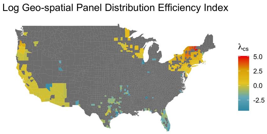
significantly depresses the local residential solar share of electrical consumption, helping
explain the relative inefficiency of the aggregated geo-spatial distribution of residential
solar across the U.S.
     Given these empirical facts, we use a structural approach to show that subsidies and
rebates alone likely cannot offset the negative impact of demand for cooling services,
namely from air conditioning, on the solar share of electrical consumption. Absent the
availability of storage technology, households in sunnier, warmer areas with residential
solar may place a strain on existing grid infrastructure when they experience lapses in
insolation. During periods of low insolation, lack of storage precludes households from
using the excess electricity they produce in periods of high insolation. This could lead to
a net decline in the solar share of total consumption if households that install residential
solar also increase total electrical consumption on the margin, which our findings suggest.
It is likely that storage technology could ameliorate the downward pressure that demand
for cooling services places on the solar share. Thus, policies that subsidize and incentivize
both residential solar adoption and the installation of batteries for storage could be one
mechanism to help achieve permanent increases in the solar share and possibly lead to a
more efficient aggregate, geo-spatial distribution of panels.
     This paper proceeds as follows. In Section 2 we provide context for the questions we
explore here. In Section 3 we present model-free evidence that the aggregate, nation-wide
geo-spatial distribution of solar panels fails to efficiently take advantage of insolation in
sunny locales, and that panel-installation rebates likely are not positively contributing
to geo-spatial efficiency. Section 4 describes a structural model of household demand for
housing and electrical consumption that accounts for heterogeneity in local, solar amenity
preferences. Section 5 discusses the structural estimation procedure and corresponding
parameter estimates. Section 6 contains counterfactual experiments designed to under-
stand which factors most significantly affect the residential solar share of electrical con-
sumption and the geo-spatial distribution of solar panels. Finally, Section 7 concludes.

2 Background
Optimal adaptation and allocation of distributed solar generation is given substantial
attention in the academic literature. The natural sciences have covered a myriad of tech-
nical aspects ranging from developing user tools for optimal panel placement to forecast-
ing regional production and storage potential (Freeman et al. 2018; Sengupta et al. 2018).
Economists have investigated the direct impacts of policies intended to encourage renew-
able energy adoption. Public research and development (R&D) expenditure (Wiser and

                                             2
Millstein 2020), state and local incentives (Hughes and Podolefsky 2015), and Federal tax
expenditure (Borenstein and Davis 2016) have been scrutinized due to the contentious
nature of public discourse on energy policy.
    Other strands of the economic literature pose important questions about how to in-
corporate new renewable capacity into the electrical grid. Empirical linkages between
utilities’ transmission price schedules and adoption of distributed solar capacity have
been established at the local level (Borenstein 2017; Wolak 2018). The price effects of
zero marginal cost generation and the large fixed costs associated with solar installation
have raised concerns about optimal rate setting for both a future fully-renewable grid and
along transition paths toward such a future (Imelda, Fripp, and Roberts 2018; Heal 2020).
    Further studies have examined the welfare effects of solar adoption through the chan-
nel of pollution mitigation. Researchers have used time series data on power sector pol-
lution to quantify the degree to which social costs stemming from emissions displaced by
increased renewable generation have been avoided. The localized environmental bene-
fits are highly dependent on where new renewable capacity is installed and what form
of non-renewable electricity generation is displaced (Callaway, Fowlie, and McCormick
2018; Sexton et al. 2018). Carbon emissions’ abatement costs associated with subsidizing
the diffusion of small and utility-scale solar distribution have been studied by both aca-
demic and government bodies, but findings are wildly mixed in terms of abatement cost
estimates (see Gillingham and Stock 2018 for a recent survey).
    Additional research has gone towards better-understanding renewable energy uptake
due to differences in regional preferences over electricity generation. Nomura and Akai
(2004) and Yoo and Kwak (2009) find heterogeneity in preferences for renewable elec-
tricity in general, as well as heterogeneity in preferences for different types of renewable
sources. Heng et al. (2020) and Bakkensen and Schuler (2020) present survey evidence of
premia in individuals’ willingness-to-pay for renewables and its sensitivity to variations
in energy policy. Bollinger and Gillingham (2012) find that peer effects are significant in
determining residential solar installation patterns: a consumer is more likely to install
residential solar panels if his neighbors have also installed them.
    Building on the evidence presented in the literature, we construct a micro-founded
equilibrium model of residential solar panel demand that directly incorporates hetero-
geneous amenity preferences for local green energy generation. We combine datasets
from Stanford’s DeepSolar project and the Lawrence Berkeley National Lab (LBNL) to
form county-level estimates of residential solar generation, insolation (the amount of so-
lar radiation reaching a given area), and the lifecycle costs of residential solar electric
generation. We use these data to structurally estimate aggregate preference parameters

                                             3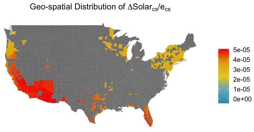
associated with housing, electrical, and the demand for residential solar panels at the U.S.
county level. This choice of model specification allows us to analyze how heterogeneity in
climatic factors and solar subsidization policies across localities affects the aggregate geo-
spatial distribution of residential solar electrical consumption across the U.S. Through the
lens of the model, we can then explore whether certain subsidization policies could lead
to a more efficient geo-spatial distribution of residential solar panels, so that the solar
share of electrical consumption is highest in sunny places where solar electricity can be
most feasibly generated.
3 A Snapshot of U.S. Residential Solar
3.1 Geographical Panel Coverage
The most granular spatial data on solar panel coverage come from Stanford University’s
DeepSolar Project measuring solar panel deployment across the United States (Yu et
al. 2018). The project utilizes machine learning techniques to analyze satellite imagery and
infer the location and surface area of small-scale solar panel installations across the lower-
48 U.S. states. The data is currently available as a static snapshot that was last updated
in December 2018. This dataset links solar panel location and surface area with average
daily solar insolation, measured in kilowatt-hours per square meter per day (kWh/m2 /d),
at the Census-tract level. Our goal here is to utilize this unique dataset to first get a general
picture of how solar panels are distributed across the U.S. We would like to understand
the degree to which the current deployment of solar panels is geo-spatially efficient, and
to understand how different policies, like rebates and grants, affect the efficient distribu-
tion.
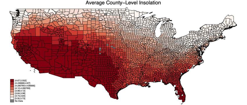
For a cursory understanding of how solar panels could be most-efficiently deployed,
Figure 1 shows a choropleth map of county-level average daily solar insolation in units
of kWh/m2 /d. This measure captures the maximum amount of energy a square meter of
SPV cells could produce over the course of the average day in a given location.23 If elec-
tricity were both storable, in say large batteries, and could freely flow across a national
network, then optimal solar panel deployment would follow the gradient featured in the
2 Themedian and mean for the 3,097 U.S. counties in the lower-48 states with available data are 4.12
kWh/m2 /d and 4.18 kWh/m2 /d respectively. Note that 19 of the 3,116 counties and county-equivalents in
the lower-48 states lacked insolation data at the census-tract level.
3 Mason County in the state of Washington has the lowest average daily solar insolation at 3.35
kWh/m2 /d, while Santa Cruz County in the state of New Mexico features 5.55 kWh/m2 /d.
4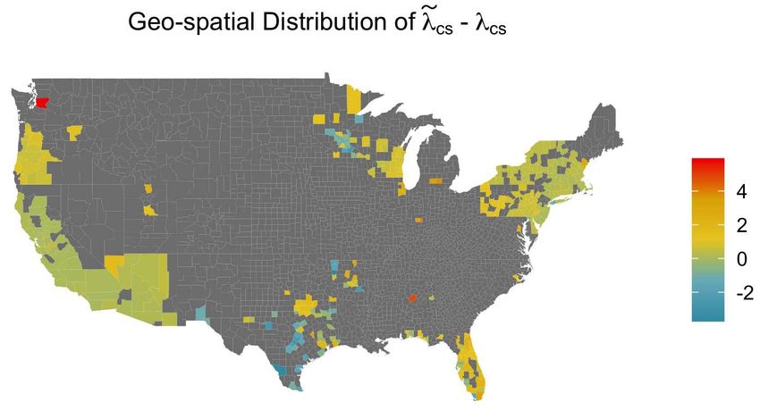
choropleth map in Figure 1.4 Under optimal allocation we would have high concentra-
tions of panels on land in the highly-irradiated Southwest and low concentrations in the
Pacific Northwest and Northeast. The electrical grid would then be structured so as to
transport this electricity from high-insolation to high-consumption locations. However,
physical restrictions (among other issues) cap cross-country transmission capacity, which
is one contributor to rich variation in the distribution of residential installations.
Figure 1: In this figure we present county-level average daily solar insolation (kWh/m2 /d)
where the colors represent octiles, with the brighter reds corresponding to places on the
map with high solar insolation. Note that the Western U.S. and Florida have climatolog-
ical conditions which contain the most relative solar-energy potential, while the Pacific
Northwest and Northeast feature the least relative solar-energy potential.
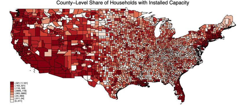
Figure 2 displays the rich dispersion in penetration of residential solar installations.5
The color gradient in this figure is divided into octiles of percentages of households at the
county level that have installed solar capacity (as of December 2018). While solar panel
uptake is highly concentrated in the Southwest wherein some counties have uptake rates
of over 10 percent, household installations are prevalent along the Eastern seaboard as
well. Despite the diffuse nature of panel uptake, daily-insolation and aggregate residen-
tial solar capacity are significantly correlated at the county level.
4 Note that optimal allocation refers only to efficiency in generation per area of SPV cells,
abstracting (for
the moment) from variation in installation costs.
5 We should note that due to lack of data on installation dates or costs in the DeepSolar dataset, for
more detailed analyses we must turn to the LBNL data which features installation data for only a subset of
American counties. Our structural model will thus ultimately operate on a smaller geographic sample than
what is presented in Figure 2.
5
Figure 2: In this figure we present the percentage of households in a given county that
feature residential solar installations. Again, the colors represent binned octiles, with
brighter reds corresponding to places with greater residential-solar uptake.

3.2 Estimating Residential Solar Generation
Unfortunately, DeepSolar, LBNL data, and administrative sources all lack direct measure-
ments of residential solar electricity generation and consumption at the county level. The
Energy Information Administration (EIA) estimates small-scale solar generating capacity
and generation at the state level using respondents’ annual estimates in form EIA-861.6
The EIA approach relies on utilities’ reporting of net-metered capacity along with dis-
tributed and dispersed resources that are not net metered. We reconcile the county-level
estimates for generation that can be inferred from the LBNL and DeepSolar data with the
state-level estimates from the EIA and construct an adjusted series at the county level.
    While DeepSolar provides estimates of panel area by household, the LBNL dataset
contains actual records of residential solar installations. Specifically, LBNL catalogs 1,456,836
observations of residential solar installations between 1998 and 2018. Among the resi-
dential observations, 1,021,967 are complete observations containing all information nec-
essary to calculate the value of residential solar electricity. Observations from the states
of Utah, Maryland, Rhode Island, and Colorado are dropped, as none contain zip code
level location data. The share of residential observations missing zip codes is negligible
in other states covered in the dataset.7 Dropping other incomplete observations removes
  6 For   more details visit: https://www.eia.gov/electricity/monthly/pdf/technotes.pdf
  7 Entries missing zip codes comprise less than 1% of total residential system capacity in all other states.

                                                       6
an additional 83,799 data points from the dataset.8
    To calculate average household solar generation at the county level, we use the LBNL
data, which contains records of both panel size and efficiency rating. Let i denote individ-
ual observations in a given county. Let χics denote system-level efficiency and φ̄cs denote
average daily insolation in county c. We must now convert the LBNL data, measured in
kilowatts (kW) of capacity, to panel area. As solar insolation data are recorded in kWh
per square meter per day, we must take a stand on a conversion between panel area and
power rating. Following the dimensional analysis procedure outlined in the National Re-
newable Energy Laboratory (NREL)9 solar module, we calculate effective panel area as
follows:

                                                           1m2   1
                               Panel Areaics = Ratingics ×     ×
                               |   {z      } | {z } 1kW χics
                                      m2               kW

With area in hand we can calculate the annual solar generation by each system in kilowatt-
hours per year.

                       solarics = Panel Areaics × χics × φ̄cs ≡ Ratingics × φ̄cs

For panels missing an efficiency listing (approximately 25 percent of observations), we
use the median efficiency rating for all panels installed that year, in that state10 . Obser-
vations that are almost certainly coded incorrectly (negative efficiency values) are also
dropped at this point. Average household solar generation at the county level, solarcs
is then taken as the total generation of solar energy from residential systems across all
households, divided by the total number of households in county c, HHcs .

                                                            HHcs
                                                    1
                                       solarcs =
                                                   HHcs     ∑      solarics
                                                            i =1

Since consumers have no control over the weather, they have no control over φ̄cs , so we
   8 After dropping observations due to incomplete observations from either missing geo-spatial indices or
missing pricing variables as described in Section 3.4, we have enough data to compute empirical aggregates
of residential solar panel electrical generation for 372 U.S. counties. The counties that remain after selection
are the non-gray counties in Figure 3.
    9 https://pvwatts.nrel.gov/pvwatts.php
  10 Refining the replacement efficiency to state level or using a broader national median does little to affect

the interpolation here.

                                                       7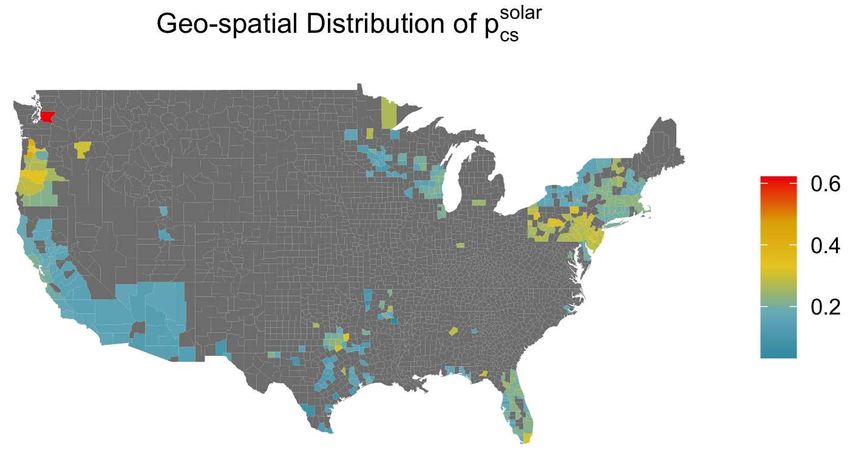
ultimately care about the average panel rating, which is just:

                                                         HHcs
                                       solarcs    1
                        Ratingcs =
                                         φ̄cs
                                               ≡
                                                 HHcs     ∑     Panel Areaics × χics
                                                         i =1

3.3 Costs and Incentives at the County Level
Both gross cost and incentive programs for residential SPV installation display substan-
tial variation at the county level. North Carolina State University’s DSIRE program indi-
cates there have been 565 regulatory policies or financial incentives put in place since the
year 2000 at the state and local level.11 Regulatory actions that incentivize SPV uptake
include easements for household installations, right-to-install laws, net metering, build-
ing requirements, and expediting permits. Financial incentives typically take the form of
production-based incentives (subsidies that are determined based on households’ gener-
ation level) or one-time transfers, such as rebates, grants, or tax credits.
    Observations in the LBNL Tracking the Sun dataset record three fiscal incentives: 1)
rebate or grant programs (R); 2) Performance-Based Incentives (PBI); 3) Feed-In Tariffs
(FIT). We observe the magnitude and duration of these fiscal instruments for over 1 mil-
lion residential SPV installations since 2000. Additional consideration is given to the In-
vestment Tax Credit (ITC): households that installed panels between 2006 and 2020 may
claim 30% of costs as a tax credit against federal income taxes.12
    While PBI and FIT subsidies are very limited (only 0.0002% of our sample are observed
to have received positive FIT and only 0.2% positive PBI), one-time installation rebates
have been widely deployed to incentivize residential solar uptake. Figure 3 shows the
geo-spatial distribution of average rebates R b cs less local taxes T
                                                                    bcs associated with panel
purchase and installation by county from the LBNL data selected after cleaning.13 Coun-
ties in Florida and Texas feature the greatest level of rebates. Given this, we would ex-
pect excess residential panel uptake conditional on production potential relative to what
would otherwise be predicted, but that is not what we observe. In Section 3.5 we con-
struct an index that characterizes the geo-spatial efficiency of residential solar installa-
tions across the U.S. Relative to counties in the west and northeast, we will show that
despite large rebates, counties in Texas and Florida have an excess supply of un-tapped
solar potential given conditionally lower rates of panel installation.
  11 See   https://programs.dsireusa.org/system/program.
  12 See https://www.energy.gov/eere/solar/downloads/residential-and-commercial-itc-factsheets.
  13 The grey counties in Figure 3 do not contain enough installation observations to accurately estimate the

local value of residential solar panels.

                                                     8
b cs − T
Figure 3: Here, we present average rebates less local sales taxes, R bcs , by county
in nominal dollars. Net rebates are highest in Texas and Florida, though King County
Washington (home of Seattle) also has offered relatively high net rebates over the past
couple of decades.
Data from LBNL are also robust on the cost side. All observations contain incentive
structure data, installation prices and system size along with either reported or estimated
sales taxes collected by local governmental authorities. This gives us a direct measure of
the tax-inclusive cost of installation, allowing for a measure of total cost for each observa-
tion. Assuming a maximal uptake of ITC claims by households contributes an additional
$9.5 billion to subsidies over this period. Under the maximal ITC claims assumption, the
combination of rebates and tax expenditures amount to greater than 64 percent of total
residential SPV installation costs, tax inclusive, during the first decade of the 2000s. In the
next section we will use the rebate, tax, and cost information featured in the LBNL data
to estimate a price index that describes the local, county-level value of residential solar
electrical consumption.
3.4 Constructing the Price of Solar Energy
To construct the implicit price of one kWh of energy derived from residential solar, we
must account for local subsidization policies, as well as the rate of long-run depreciation
9for SPVs.14 The LBNL dataset allows us to account for these factors under a couple of
assumptions. Specifically, we calculate psolar cs at the county level using a levelized cost
of energy (LCOE) approach, following a simplified version of Flowers et al. (2016). The
LCOE is the ratio of the present value of lifetime net expenditures (costs minus subsidies)
to the present value of electricity generation (the sum of lifetime discounted generation).
The LBNL dataset provides data on installation costs, sales taxes, lump-sum rebates or
grants, and levels and durations of FIT/PBI programs. The remaining parameters re-
quired to calculate LCOEs are assigned according to established values in the literature.
We assume a 30-year lifespan for panels, a 1% annual depreciation rate (DR), an annual
cost of maintenance equal to 1% of fixed costs (Cics ), and a discount rate of 3% (r), in line
with Jordan and Kurtz (2013) and Flowers et al. (2016). Further, lacking data on whether
or not individual households used ITC tax credits, we construct two separate solar price
variables. In the first, which we use in our primary structural estimation and counterfac-
tual exercises, we construct psolar
cs under the assumption that ITC uptake is zero. In the
second, we allow for maximal uptake of ITC. Estimates of our structural model under the
two different price indices are similar, so we do not perform counterfactual analyses with
the price indices where ITC uptake is assumed maximal.
Price construction induces further sample selection that, after aggregation, gets us to
the final count of 372 counties containing usable aggregate solar demand observations.
Many panel installation observations from the LBNL data are missing entries for either
the installation price, whether a grant/rebate for the installation was received, or the
amount of FITs and PBIs. The incidence of missing price variables varies greatly among
states, and comprises about 25% of all observations. The states of Ohio, New Mexico,
Montana, Kansas, and the District of Columbia feature all observations that are missing
at least some of the required pricing variables, so we drop these states from our sample.
To allow us to keep a larger share of the remaining observations missing price data, we
assign average LCOEs at the county-year level to observations in that same county that
are missing prices. Finally, we also drop counties for which psolar
cs is implied to be negative.
This can happen as a result of observing very few installations, all of which are highly
subsidized, thus forcing LCOEics < 0.
In addition to fixed costs Cics , let Tics represent local sales taxes, and let Rics be the
one-time local rebate received upon installation. LCOEs must be calculated to account
for the fact that FITs and PBIs expire after so many periods. The rates and dates of expiry
depend on local policies as well as when the panel system was acquired by the consumer
14 This price encodes the net present value of one unit of residential solar energy consumed, accounting
for all possible costs associated with purchasing, installing, and maintaining the panels.
10and, sometimes, whether or not the consumer filed the necessary paperwork to receive
FIT be the number of periods after which FITs expire and
FIT and/or PBI credits. Let τics
PBI be the number of periods after which PBIs expire. Given a 30-year lifespan, the
τics
LCOE is:
LCOEics =
0.01×Cics τ FIT FITt (1− DR)t solarics τ PBI PBIt (1− DR)t solarics
Cics + Tics − Rics + ∑29
t=0 ( 1 +r ) t
− ∑t=ics0 ( 1 +r ) t
− ∑t=ics0 ( 1 +r ) t
(1)
t
(1− DR) solarics
∑29
t=0 ( 1 +r ) t
Figure 4: In this figure, we present a choropleth map of estimated local solar prices, as-
suming 0% ITC uptake. High φcs and Rics weigh negatively on LCOEics , thus driving
down solar prices. Despite high rebates, King County Washington also is associated with
the highest price of solar due to very low solar insolation.
g cs be the total number of household-level panel installation observations for
Let HH
county-state unit c, s. Note that HH g cs ≤ HHcs always, since we cannot observe more
households with installed solar capacity than the total number of households that exist in
g cs < HHcs , strictly. Let τeics be the
the county. In fact, it is always true in our data that HH
year in which agent i who lives in county-state c, s purchased and installed solar panels.
We calculate county-level average solar prices as the average of LCOE values across all
11installed units (converted to $2018) and over time, weighted by system size Sics :
g
HH cs p2018
∑2018
t=2000 ∑i =1 1 (τ
eics = t) Sics LCOEics pt
psolar
cs = g
(2)
HH
∑2018 cs
t=2000 ∑i =1 Sics
Sums start at t = 2000 since that is the first year in our sample. pt is the Consumer
Price Index for All Urban Consumers (CPI-U) from the Bureau of Labor Statistics. In
our baseline estimation, where we assume ITC uptake is zero, Rics contains only local
rebates. When we assume ITC uptake is maximal, we adjust Rics to include 30% of costs
— 0.3 × Cics .
Figure 4 presents the geo-spatial distribution of solar prices. Given the LCOE calcu-
lations in (1), rebates weigh negatively on the price. Notice that despite issuing average
net rebates of over $10,000, King County, Washington (home to Seattle) is also associated
with one of the highest effective solar prices, due to the combination of both high instal-
lation costs and low average daily insolation, φcs . Since solarics = Ratingics × φcs , low
φcs puts upward pressure on LCOE, and high φcs puts downward pressure on LCOE.
We see similar trends with respect to Oregon, which offers few rebates but also has low
φcs driving prices up. Pennsylvania, also, offers relatively high subsidies (around $10,000
on average), and yet features relatively above-average solar prices due to relatively low
daily insolation.
Examining variation between the geo-spatial net rebate and price distributions leads
to a couple of questions. Rebates in cloudy places like Seattle seem poorly targeted from a
national perspective, even though local policymakers may prefer them. Can we construct
a measure of geo-spatial efficiency in order to understand where there may be surpluses
or shortages of installed panels, relative to other localities? In the next section, we pro-
pose such an index. Second, given such potential aggregate, national inefficiencies, do
local rebates contribute to a more efficient geo-spatial distribution of residential panels,
relative to a no-rebate environment? We explore this second question with our structural
counterfactuals in Section 6.
3.5 Geo-spatial Efficiency of Residential Coverage
As previously mentioned, the most efficient distribution of solar panels would see great
concentrations of residential solar generation in the Southwest and West with sparser
concentration in cloudier places like the Pacific Northwest and Northeast. However, vari-
ation in local subsidization of solar electricity and solar installation costs may incentivize
consumers in places with relatively low average solar insolation to engage in relatively
12high rates of solar adoption. For this reason, we seek a measure of the degree to which the
current distribution of residential panels across the U.S. deviates from the efficient distri-
bution, which would follow the geo-spatial gradient in Figure 1, absent consideration for
transmission frictions across a fractured electrical grid.
The share of average residential electrical consumption in county-state unit c, s that is
attributed to residential solar is given by:
Ratingcsφcs solarcs
µcs = ≡
ecs ecs
where ecs is per-household total electrical consumption and µcs ∈ [0, 1), allowing for no
residential solar consumption but requiring that some fraction of electrical consumption
always comes from other sources. Let C be the number of county-state pairs in our sam-
ple. We can compare the residential solar market share of electrical consumption across
these counties using the empirical distribution function:
1
Pµ (m) =
C ∑ ∑ 1µcs ≤m
s c
We can also rank counties in terms of their average daily solar insolation:
1
Pφ (ϕ) =
C ∑ ∑ 1φcs ≤ϕ
s c
Using both of these statistics, we construct a unit-less index on the log-scale that char-
acterizes the degree to which the geo-spatial distribution of residential solar panels devi-
ates from the efficient distribution:
Pµ (µcs = m)
λcs = ln (3)
Pφ (φcs = ϕ)
If λcs > 0 then county-state c, s has excess installed residential solar capacity relative to
the other counties in our sample. If λcs < 0 then county-state c, s has an excess supply of
un-tapped solar potential relative to the other counties in our sample.
Note that the moments of the distribution of λcs provide rich summary statistics char-
acterizing how the geo-spatial distribution deviates from the efficient distribution. As
E(λcs ) → 0 and Var(λcs ) → 0 simultaneously, the distribution of λcs converges to the
efficient distribution. If E(λcs ) = 0 and Var(λcs ) > 0 then the distribution is ineffi-
cient yet unbiased. That is, geo-spatial inefficiency is equally attributable to excess sup-
ply in cloudier places and relative shortages in sunnier places. If E(λcs ) , 0 but finite,
13Figure 5: The geo-spatial distribution of the log efficiency index, λcs , shows that relative
excess residential-solar supply is concentrated in the Northeast, while relative residential-
solar shortages are concentrated primarily in Texas and Florida. The mean efficient
county in our sample is Tuolumne County near Yosemite National Park in Central Cali-
fornia.
then necessarily Var(λcs ) > 0, and the distribution is both inefficient and biased. If
E(λcs ) < 0 then, generally speaking, residential solar capacity is inefficient due more
to under-installation in sunnier states relative to the efficient distribution. If E(λcs ) > 0
then, generally speaking, residential solar capacity is inefficient due more to excess solar
capacity in cloudier states relative to the efficient distribution.
After the sample selection procedures discussed in the previous sections, we can com-
pute the geo-spatial distribution of λcs for the counties that survive our selection proce-
dure. This geo-spatial distribution is presented in Figure 5, where redder counties fea-
ture a relative over supply of panels, while bluer counties feature relative under sup-
ply. Notice that over supply appears concentrated in the Northeast and Pacific North-
west, while counties in Texas are associated with a notable under supply considering the
above average solar insolation levels these counties experience. With respect to the dis-
tribution of λcs , we find that the mean is not significantly different from zero, though
Var(λcs ) = 2.164 > 0, suggesting an unbiased but inefficient distribution of solar panels.
144 Model of Household Demand
The model we propose operates at the U.S. county level. Index county units by c ∈ C.
Each county belongs to a state s ∈ S. A consumer-unit i in county c and state s has
basic consumption preferences over housing hics (in units of square feet), total household
electrical consumption eics which includes solar (in units of kWh), an additional amenity
preference for consumption characterized by the panel rating variable Ratingics (in units
of kW, not kWh), and an outside commodity cics which captures all other consumption.
All choices are assumed to be strictly positive and continuous, and all consumers are
assumed to be price takers, meaning that their atomic decisions have negligible influence
on general-equilibrium outcomes. In our preference formulation consumers have control
over the overall kilowatt-rating of the panels they purchase but not their total output,
which also depends on local insolation. The household decision environment is a static
one: we do not consider savings or investment decisions but rather account for the long-
run effects of solar-panel investment by constructing prices accordingly, as previously
described. The goal of our modeling exercise is to find reasonable estimates of structural
demand parameters in order to explore how both local and national subsidization policies
may contribute to the inefficient geographic distribution of solar capacity.
We do not distinguish between electricity consumed from solar versus other sources.
Instead, consumers prefer to consume solar electricity only because they have preferences
for the solar amenity. That is, they like solar perhaps because they are environmentally
conscious or enjoy the feeling of self-reliance derived from consuming electricity pro-
duced with equipment they own. However, a consumer, when in the act of consuming
electricity to power appliances or lights, for example, does not care about the source of
electricity. In this sense we assume that the solar amenity preference and preferences for
consumption are somehow separable in utility.
The preference structure we impose is of the nested constant elasticity of substitution
(CES) variety. Our nesting structure features a three-tiered hierarchy. To allow for the fact
that housing consumption and electrical consumption may be complementary, we allow
them to be contained within their own nest. The next layer accounts for complementari-
ties between the composite of housing and electrical consumption and the solar amenity.
Finally, the outer-most layer accounts for the relationship between housing/electrical
15consumption plus the solar-amenity composite and all other consumption:
ucs (hics , eics , Ratingics , cics ) =
" κρ # κ1
αρ
γ hαics + (1 − γ )eαics + ηcs ( Ratingicsφcs )ρ + cκics , (4)
α , ρ, κ , 0 and α , ρ, κ < 1
α governs the degree to which housing and electricity are complementary. ρ governs the
substitutability between the housing/electricity composite good and the solar amenity. κ
governs the rate at which consumers substitute between all other consumption and the
housing/electricity plus solar-amenity composite. γ governs the relative importance con-
sumers place on housing versus electrical consumption. ηcs characterizes the degree to
which local demographic, political, cultural, and climatic factors impact solar consump-
tion preferences. Note that all consumers in the same county-state unit face the same
amenity-preference weight ηcs . We assume that consumers value electricity indepen-
dently of where it comes from but care about solar-panel-generated electricity only as an
amenity. That is, they do not separately choose non-solar and solar electrical consump-
tion. This assumption reflects the difficulty in decomposing electrical consumption from
solar versus non-solar due to grid-based electricity comprising flows from both sources.
All households in the same county-state unit face the same market prices. Let pcs h be
the average price per square foot of owner-occupied housing, as reported in the 2014-
2018 American Community Survey (ACS) 5-year estimates. Let pecs be the market price
per kilowatt hour of electricity in county c and state s. Let psolar
cs be the net-present-value
of solar electricity consumption, accounting for wear-and-tear and depreciation of panel
efficiency.15 pccs is a price index describing the value of all other consumption. Let yics en-
code total income net of savings for household i in county c and state s. The household’s
budget must satisfy
h
pcs hics + pecs eics + psolar c
cs Ratingicsφcs + pcs cics
(5)
≤ yics + max{ pecs ( Ratingicsφcs − eics ), 0}
Within a county-state unit, the exogenous source of household heterogeneity is thus lim-
ited to yics . Note that in most localities, excess electricity generated from residential so-
lar panels is sent back to the grid, and the household is offered a credit at par with the
market-value of excess production, hence the final term on the right-hand-side.
15 This is the solar price constructed in Section 3.4.
16Since all household heterogeneity within a particular county-state unit is governed by
exogenous variation in income, we can exploit the homotheticity of ucs to focus solely on
the problem of a representative consumer, given ucs is associated with an indirect utility
function that satisfies the polar form of Gorman (1959). Further, since we observe that
∑i ( Ratingicsφcs − eics ) < 0 in all county-state combinations in our sample, it follows that
no county produces more residential solar electricity than the total amount of electricity
it consumes. Thus, we can safely ignore the argument max{ pecs ( Ratingicsφcs − eics ), 0} on
the right-hand side of the representative consumer’s budget constraint when characteriz-
ing aggregate demand properties in the next section. From here on, we drop i subscripts.
Moving forward, we will let choice variables that are missing their i subscripts correspond
to aggregate demands for county c in state s.
4.1 Equilibrium Aggregate Demand
The representative consumer in county c and state s solves:
max ucs (hcs , ecs , Ratingcs , ccs )
hcs ,ecs ,Ratingcs ,ccs
h
subject to pcs hcs + pecs ecs + psolar c
cs Ratingcsφcs + pcs ccs ≤ ycs
In equilibrium, the marginal rate of substitution between housing and total electrical con-
sumption is:
α −1 h
γ hcs pcs
= e (6)
1−γ ecs pcs
The marginal rate of substitution between consuming the solar amenity and total electric-
ity is:
ρ
ηcsφcs Ratingρcs−1 psolar
cs φcs
ρ−αα = (7)
γ hαcs + (1 − γ )eαcs (1 − γ )eαcs−1 pecs
Given the separability between the nest which includes hcs , ecs , and Ratingcs and ccs , we
can fully characterize the demand for housing, electricity, and solar panels without a need
to specify equilibrium first-order conditions for ccs . Indeed, separability between Ratingcs
and the housing/electricity nest allows us to substitute out hcs from (7) using (6) in order
to arrive at an expression that roughly characterizes the fraction of electrical consumption
17devoted to solar:
ρ−1 ρ h α ! αα−ρ
Ratingcs ηcsφcs pcs (1 − γ ) α−1 psolar
cs φcs
γ e
+ 1 − γ = (8)
ecs 1−γ pcsγ pecs
(8) can be used in order to arrive at consistent estimates of the structural parameters,
given data for prices, demand, and average daily insolation by county. (8) is thus our
primary structural estimating equation around which we will form a likelihood function
and arrive at estimates of α , ρ, γ and a residual expression for the amenity weight ηcs .
Given κ does not factor into our primary estimating equation, which characterizes the
marginal rate of substitution between housing/electricity and the solar amenity, we need
not estimate this parameter, so it remains free. In the following section, we provide the
details of our structural estimation approach, while also addressing the orthogonality
assumptions required for consistent recovery of the parameters.
5 Structural Estimation Procedure
Our estimation procedure operates on county-level data for 372 counties, distributed
mostly in the western U.S., northern Midwest, Texas, Florida, and the northeastern U.S.
We select a sample of counties for which we have sufficient data on residential solar panel
installations, including cost of installation and any rebates, feed-in tariffs, or performance-
based incentives received by the household, where county selection is as described in
Section 3.
The primary equation we target is a logged version of (8), controlling for local demo-
graphic, economic, and environmental factors that may be correlated with the amenity
weight, ηcs . Our approach is to form a likelihood function around (8) while placing prior
distributions (flat, where possible) on the structural parameters, ρ, α , and γ , as well as the
likelihood variance σ 2 , in order to estimate the posterior distribution of model parame-
ters given data. We thus take a Bayesian approach to estimation and use Monte Carlo
integration techniques to estimate the posterior distribution. Specifically, we estimate
the posterior distribution using a Hamiltonian Monte Carlo (HMC) method as described
in Neal (2011). We run four different versions of the estimation procedure, separately
restricting ρ and α to either be in (0, 1) or (−∞, 0). We then employ model selection
techniques to compare the log-posterior predictive density functions of the separately-
estimated models, where sampling from the predictive distribution is undertaken using
the leave-one-out methods described in Vehtari, Gelman, and Gabry (2017).
18The estimation results presented in the main text involve estimates of the solar price
index where, lacking data, we assume that uptake of federal ITC is zero. In Appendix
A we present estimation results under the alternative assumption that ITC uptake is the
maximum 30% for all observed installations. There is no significant discernible difference
between the posterior distribution results under either price-construction assumption,
so we dispense with performing counterfactual analyses on the model where psolar cs is
constructed allowing for 30% ITC uptake.
Our parameter estimates and model selection procedures suggest that ρ ∈ (0, 1), so
that the solar amenity and the housing/electricity composite are substitutes. We also pre-
fer the model where α < 0, which we believe to be consistent with theory: we expect
housing and electricity to be complementary since larger houses are to be associated with
more appliances, more lights, and more space to heat and cool, and thus greater electrical
consumption. Controlling for local demographic, political, cultural, and climatic factors,
we find no significant relationship between solar demand and either population den-
sity, median household income, or rates of home ownership. We find that counties with
higher shares of Republican voters (GOP voting share) are somewhat surprisingly asso-
ciated with greater preferences for the solar amenity. Meanwhile, the number of cooling
degree days is the most significant local factor weighing down on solar amenity prefer-
ences. We discuss all of these findings and present robustness tests to check for regressor
endogeneity in the sections that follow.
5.1 Likelihood and Prior Distributional Assumptions
Taking logs of (8) and isolating the log of the amenity weight as a residual, ln ηcs , we get:
psolar
cs Ratingcs
ln + (1 − ρ) ln + (1 − ρ) ln φcs + ln(1 − γ )
pecs ecs
h α ! (9)
ρ −α pcs (1 − γ ) α−1
+ ln γ + 1 − γ = ln ηcs
α pecsγ
We expect the amenity weight ηcs to be correlated with local demographic, economic,
and environmental factors, such as population density, median household income, polit-
ical preferences, and the number of hot versus cold days during the year. We thus write
19ln ηcs as a linear function of the following set of controls:
ln ηcs = β1 ln pop densitycs + β2 ln GOP voting sharecs
+ β3 ln median incomecs + β4 ln heating dayscs
+ β5 ln cooling dayscs + β6 ln homeownership ratecs + ǫcs
Population density is from the 2011-2015 ACS 5-year estimates. The GOP voting share
variable measures the share of the vote the Republican candidate, Donald Trump, re-
ceived in the 2016 presidential election. Median income is the median income of a home-
owning household, not a person, from the 2014-2018 ACS 5-year estimates. Heating and
cooling degree days are measures which quantify a given locale’s demand for energy
to heat and cool buildings, depending on the region’s daily outdoor air temperature.16
These variables are found in the DeepSolar data along with φcs . The homeownership rate
describes the fraction of all households that are owner-occupied, as found in the 2011-
2015 ACS 5-year estimates. ǫcs is the idiosyncratic residual that is assumed iid across
county-state observations. We form the likelihood function around this error term, which
is assumed normally distributed, and the variance of which is given a conjugate inverse
gamma prior:
ǫcs ∼iid N (0, σ 2 )
σ 2 ∼ InvGamma(5, 5)
The structural preference parameters ρ and α are given priors that depend on whether
we ex-ante (prior to running the integration procedure) restrict ρ and/or α to be in the
unit interval or negative:
ρ, α ∼ U [0, 1], if either ρ and/or α ∈ (0, 1)
1
− ρ, −α ∼ LN − , 1 , if either ρ and/or α < 0
2
U is the uniform distribution and LN is the log-normal distribution. Note that we run
four separate estimations accounting for the fact that both ρ and α may be positive, one
is negative and the other is positive, or both are negative.
16 To compute heating degree days, for example, take a region’s average temperature on any given day
and subtract it from a pre-set base temperature, which is effectively the constant building temperature that
is desired. This constant temperature is attributed to local building standards and is typically taken to be
18.3◦ C (65◦ F) in the United States. If this value is positive, then the value gives the number of heating
degree days. If it is negative, the absolute value yields the number of cooling degree days.
20The contribution of housing consumption to the housing/electricity preference nest is
given by γ . Having found in simulations that this parameter often piles up at its upper
bound of 1, we impose an informative beta prior on γ :
γ ∼ Beta(1, ω)
ω is a hyper-parameter which we estimate by taking logs of the infra-marginal rate of sub-
stitution between solar and electrical consumption in (6) and running an OLS regression
to get a prior estimate for γ which we call γb. We allow this prior estimate to correspond to
the mean of the beta distribution, which gives us ω b = 1/γb − 1. This value is ωb = 0.289.
Finally, the contribution of control variables to the amenity weight is governed by the
vector β with components β j . We give these parameters flat, improper priors, allowing
them to take any real value with equal quasi-probability:
β j ∼ U (−∞, ∞), ∀ j ∈ {1, 2, 3, 4, 5, 6}
While improper priors can sometimes create computational issues when sampling, con-
vergence criteria for our integration schemes are all satisfied and no such issues arise.
5.2 Posterior Distribution Estimates and Model Selection
Table 1: Model Selection Assessments
Model el ppd Differencea S.E. Differenceb
ρ, α ∈ (0, 1) — —
ρ ∈ (0, 1), α < 0 -11.2 3.3
ρ < 0, α ∈ (0, 1) -797.5 21.8
ρ, α < 0 -799.0 21.7
a This is the difference in the expected log-posterior predictive
density relative to the model with the highest el ppd value —
ρ, α ∈ (0, 1). As long as the absolute value of the el ppd
difference is several times the standard error of the differences,
we can be confident that the baseline model provides a better
fit than its alternatives (Vehtari, Gelman, and Gabry 2017).
bThis is the standard error of the posterior differences across
HMC sample draws.
21The structural models, conditional on prior assumptions regarding how the solar
amenity, housing, and electricity are related (substitutes versus complements), are es-
timated using an HMC integration routine parallelized over four independent chains.
Each chain generates 8000 samples from the posterior distribution of parameters condi-
tional upon prior assumptions and data. We allow the first 4000 samples to be considered
warm-up/burn-in samples and drop them from our posterior analyses, leaving us with
4000 × 4 = 16000 sample parameter vectors for each model. The operations required to
perform the HMC take approximately 20 minutes on a standard multi-threaded, multi-
core laptop. All four models converge according to the R b convergence criterion for HMC
estimation procedures, as outlined in Vehtari et al. (2019).17
Tables 2 and 3 present the posterior distribution estimates of the model’s structural
parameters, under the respective assumptions that ρ ∈ (0, 1) and ρ < 0. The top half of
each table contains estimates under the assumption α ∈ (0, 1), while the bottom half of
each table contains estimates assuming α < 0. We perform model selection by assessing
the expected log posterior predictive density (el ppd) using the leave-one-out sampling
method as described in Vehtari, Gelman, and Gabry (2017). el ppd is largest for the model
with ρ, α ∈ (0, 1), though for theoretical reasons we prefer the model where ρ ∈ (0, 1)
and α < 0, allowing housing size and electrical consumption to be complements. As can
be seen in Table 1 the model with ρ, α ∈ (0, 1) is only weakly preferred, in terms of el ppd
to that with ρ ∈ (0, 1) and α < 0, relative to the two models where ρ < 0. Since both
models where ρ ∈ (0, 1) are strongly preferred, in terms of el ppd to those where ρ < 0,
solar demand and demand for housing/electrical consumption are substitutes. Further
evidence that the ρ ∈ (0, 1) models provide better fitness can be seen by comparing the
likelihood variances σ 2 in Table 2 to those in Table 3. The likelihood spreads are substan-
tially larger in the complements models with ρ < 0. The log-posterior densities V (P ) are
also larger in models with ρ ∈ (0, 1), so that the posterior is tighter and more concen-
trated than the estimated distributions in models with ρ < 0. For all of these reasons, we
focus our analyses on the estimates in Table 2.
b statistics for all model parameters as well as the same statistic associated
17 The criterion states that if the R
with estimates of the log posterior density V (P ) are approximately unity, then the numerical integration
routine has converged to the true posterior distribution. The R b statistic used to assess HMC integration con-
vergence should not be confused with (and is unrelated to) the R2 statistic used by frequentists in ANOVA
tables.
22Table 2: Posterior Distribution Estimates, ρ ∈ (0, 1)
α ∈ (0, 1)
Parameter b
R Mean S.D. 2.5% 25% 50% 75% 97.5%
ρ 1.000 0.951 0.007 0.937 0.946 0.951 0.955 0.965
α 1.001 0.748 0.106 0.473 0.701 0.772 0.822 0.883
γ 1.000 0.967 0.027 0.900 0.963 0.974 0.980 0.987
σ2 1.000 0.104 0.008 0.090 0.099 0.104 0.109 0.121
β1 1.000 0.010 0.024 -0.037 -0.006 0.010 0.026 0.058
β2 1.000 0.181 0.063 0.056 0.138 0.181 0.224 0.304
β3 1.000 -0.034 0.073 -0.176 -0.082 -0.034 0.014 0.110
β4 1.000 -0.104 0.038 -0.177 -0.129 -0.104 -0.078 -0.029
β5 1.000 -0.419 0.074 -0.565 -0.469 -0.419 -0.370 -0.271
β6 1.000 -0.171 0.146 -0.455 -0.269 -0.173 -0.073 0.118
V (P ) a 1.001 235.024 2.363 229.397 233.735 235.397 236.736 238.531
αTable 3: Posterior Distribution Estimates, ρ < 0
α ∈ (0, 1)
Parameter b
R Mean S.D. 2.5% 25% 50% 75% 97.5%
ρ 1.000 -0.011 0.005 -0.022 -0.013 -0.010 -0.007 -0.004
α 1.000 0.570 0.264 0.049 0.361 0.618 0.799 0.952
γ 1.000 0.784 0.257 0.095 0.688 0.915 0.963 0.994
σ2 1.001 5.872 0.442 5.071 5.561 5.849 6.159 6.805
β1 1.000 -0.186 0.174 -0.528 -0.304 -0.185 -0.065 0.153
β2 1.000 -1.361 0.469 -2.280 -1.676 -1.356 -1.049 -0.435
β3 1.000 0.722 0.518 -0.296 0.371 0.718 1.070 1.746
β4 1.000 -0.324 0.278 -0.873 -0.512 -0.319 -0.137 0.221
β5 1.000 -2.196 0.529 -3.234 -2.552 -2.192 -1.837 -1.173
β6 1.000 3.202 1.121 1.009 2.459 3.209 3.957 5.405
V (P ) a 1.000 -540.145 2.632 -545.942 -541.733 -539.940 -538.316 -535.571
αing the prior on α appears to most significantly impact inference regarding the housing weight γ and the contribution of the control variables to amenity preferences β. One rea- son we prefer the model where α < 0 is that in that model γ
You can also read