Arbitrary Angle of Arrival in Radar Target Simulation - arXiv
←
→
Page content transcription
If your browser does not render page correctly, please read the page content below
1

                                                                            Arbitrary Angle of Arrival in
                                                                              Radar Target Simulation
                                                    Axel Diewald, Graduate Student Member, IEEE, Benjamin Nuss, Graduate Student Member, IEEE
                                                                    Mario Pauli, Member, IEEE and Thomas Zwick, Fellow, IEEE

                                             Abstract—Automotive radar sensors play a key role in the                    deceive a radar under test (RuT) by creating an artificial
                                          current development of autonomous driving. Their ability to                    environment comprising of virtual radar targets. In order for
                                          detect objects even under adverse conditions makes them indis-                 this environment to be as credible and realistic as possible,
                                          pensable for environment-sensing tasks in autonomous vehicles.
arXiv:2106.12308v2 [eess.SP] 6 Jul 2021

                                          The thorough and in-place validation of radar sensors demands                  the virtual radar targets must be generated as accurate as
                                          for an integrative test system. Radar target simulators (RTS) are              possible in regards of their characteristics. Recent RTS systems
                                          capable of performing over-the-air validation tests by creating                have already achieved a setting point precision higher than the
                                          artificial radar echoes that are perceived as targets by the                   resolution of common and even future radars in terms of range,
                                          radar under test. Since the authenticity and credibility of these              Doppler and radar cross section (RCS) [7]–[10]. Nonetheless,
                                          targets is based on the accuracy with which they are generated,
                                          their simulated position must be arbitrarily adjustable. In this               the simulation of the angle of arrival (AoA) in current RTS
                                          paper, a new approach to synthesize virtual radar targets at                   systems has yet to meet the angle estimation capabilities of
                                          an arbitrary angle of arrival is presented. The concept is based               their counterpart. By electronically switching between discrete
                                          on the superposition of the returning signals of two adjacent                  and fixed angular positions the azimuth dislocation of a virtual
                                          RTS channels. A theoretical model describing the basic principle               radar target can be simulated [7], [11], which, however, does
                                          and its constraints is developed. Additionally, a measurement
                                          campaign is conducted that verifies the practical functionality of             not satisfy the angular accuracy capabilities of modern radar
                                          the proposed scheme.                                                           sensors. Another approach is to mechanically rotate the RTS
                                                                                                                         system centric around the RuT [12]–[14], which significantly
                                            Index Terms—Radar target simulation, angle of arrival, auto-
                                          motive radar.                                                                  limits the number of virtual targets and their inherent lateral
                                                                                                                         movement speed. Rotating the RuT itself [15] results in the
                                                                                                                         same restrictions and, in addition, is not suitable for integrated
                                                                    I. I NTRODUCTION
                                                                                                                         radar sensor validation.
                                              N RECENT years the development of advanced driver
                                          I   assistance systems (ADAS) and autonomous driving has
                                          reached new levels of sophistication. For the task of sensing
                                                                                                                            Therefore, the authors present a new approach that enables
                                                                                                                         the generation of virtual radar targets with an arbitrary angle
                                                                                                                         of arrival that is neither limited in regards of the methodology
                                          the surrounding environment autonomous vehicles rely on a                      of the RTS, as it is applicable for analog and digital systems,
                                          variety of sensors, such as camera, lidar (light detection and                 nor by the modulation scheme of the RuT. The concept is
                                          ranging), ultrasound and radar. Due to its weather robustness                  based on the superposition of two neighboring virtual radar
                                          and long range capability, the latter plays a significant role for             echoes, that enables the synthesis of simulated radar targets
                                          a large share of autonomous driving functions and therefore                    at an adjustable lateral position. In the following the working
                                          needs to be thoroughly and integratively validated. Carrying                   principle of radar target simulation and the underlying signal
                                          out these validation tests in the field involves a great deal of               model will be outlined. Thereupon, the fundamental idea of
                                          effort, as distances in the order of several million kilometers                the proposed approach, as well as its constraints, calibration
                                          have to be covered to guarantee the faultless functioning of the               and disadvantages will be elaborated. Finally, the results
                                          system [1]–[3]. In addition, these tests are not repeatable since              of a measurement campaign that demonstrate the successful
                                          individual traffic situations are unique and, therefore, must be               implementation of the concept will be presented.
                                          reiterated whenever the system undergoes any design changes.
                                             For these reasons, radar target simulators (RTS) have re-
                                          cently drawn a lot of attention in research, as they provide                                 II. R ADAR TARGET S IMULATION
                                          validation capabilities to test radar sensors in-place and under                  The overall concept of the RTS is shown in Fig. 1. The
                                          laboratory conditions [4]–[6]. Their working principle is to                   RuT is placed closely in front of the RTS antenna front ends
                                            Manuscript received Month Day, 2021; revised Month Day, 2021. This work      in compliance with the far-field condition [16]. The front end
                                          was supported in part by the German Federal Ministry for Economic Affairs      modules are arranged in a semicircle formation with the RuT
                                          and Energy (BMWi) under Grant ZF4734201PO9 (Corresponding author:              as the center and equal distance between each module. The
                                          Axel Diewald.)
                                            A. Diewald, B. Nuss, M. Pauli and T. Zwick are with the Institute of Radio   receive antenna (Rx) picks up the radar signal transmitted
                                          Frequency Engineering and Electronics (IHE), Karlsruhe Institute of Technol-   by the RuT, which is thereafter down converted to a lower
                                          ogy (KIT), 76131 Karlsruhe, Germany (e-mail: axel.diewald@kit.edu).            intermediate frequency frts . Subsequently, the single target
                                            Color versions of one or more of the figures in this article are available
                                          online at http://ieeexplore.ieee.org.                                          generation modifications, namely a time delay, a Doppler shift
                                            Digital Object Identifier ...                                                and an attenuation, are applied to the signal before it is up
This work has been submitted to the IEEE for possible publication. Copyright may be transferred without notice, after which this version may no longer be
accessible.
be simulated with the help of a complex quadrature mixer [24],
[25] or through fine range discretization [26]. The attenuation
Delay can be implemented with a simple samplewise multiplication.
Doppler The delay τrts , Doppler shift fD,rts and attenuation A
frts Attenuation frts required for the virtual target generation can be derived from
the target’s range Rt , radial velocity vt and RCS σt as follows
2Rt
τrts = (1)
c0
2fc vt
fc flo fc fD,rts = (2)
c
√0
σt
A= (3)
Rt 2
where fc describes the lower bound of the radar’s frequency
Front ends band and c0 the speed of light.
B. Signal Model
Rx
In the following the radar signal that is transmitted by
Tx the RuT and modified by the RTS will be modeled. For the
sake of simplicity, a Frequency-Modulated Continuous Wave
(FMCW) radar will be assumed. Nonetheless, the underlying
principle of this approach operates independently of the mod-
ulation scheme of the radar and only the subsequent math-
ematical expressions must be adapted. The RuT’s multiple-
input multiple-output (MIMO) antenna array, comprising of
Ntx transmit and Nrx receive antenna elements, can be unified
RuT to form a virtual antenna array of size NA = Ntx · Nrx
[27]. As will later be shown, the signal delay’s impact on the
Fig. 1: Concept of the radar target simulator signal phase, plays a key role for the success of the proposed
concept. For this reason, the following analytical descriptions
focus primarily on the signal phase in order to facilitate the
converted back to its original carrier frequency fc and re-
comprehension of the approach and its limitations.
transmitted towards the RuT by the front end transmit antenna The RuT transmits a signal whose frequency and phase can
(Tx). Each RTS front end pair is coupled with its own signal be described in regards of time t ∈ [0, T ] as
modification module enabling an independent target generation
for each RTS channel. B
ftx (t) = fc + · t (4)
Z tT
B 2
A. Target Generation ϕtx (t) = 2π f (t0 ) · dt0 = 2π fc · t + ·t (5)
0 2T
RTS systems can be divided into analog or digital in terms
of their target generation methodology. Since the approach where B is the signal’s bandwidth and T the chirp period.
presented in this paper can be implemented with either one, The radiated signal travels through free space, is received by
both system domains are shortly explained. one of the RTS front ends and down converted, causing a time
Analog RTS systems utilize optical or electrical delay delay τtx and a phase shift of ϕlo (t) = 2πflo · t and can be
lines [17]–[19], surface acoustic wave (SAW) filters [20], or expressed as
frequency mixers [5], [21] to simulate the target’s range. The ϕrts,rx (t) = ϕtx (t − τtx ) − ϕlo (t)
required Doppler shift can be applied with a vector modulator
B
2
[4], [22], with a digitally controlled phase shifter [23], or by = 2π −fc τtx + frts · t + (t − τtx ) (6)
2T
applying a frequency offset to the local oscillator for the up
and down conversion [17]. A variable gain amplifier can be where frts = fc − flo describes the signal’s down converted
employed for the simulation of the RCS. lower bound frequency. The RTS generates a virtual radar
Digital RTS systems, on the other hand, perform the tar- target by applying an artificial delay τrts . Subsequently, the
get generation task utilizing a field-programmable gate ar- signal is up converted to its carrier frequency
ray (FPGA) after a preceding analog-to-digital conversion. ϕrts,tx (t) = ϕrts,rx (t − τrts ) + ϕlo (t)
Within the FPGA the radar signal is either analyzed and re-
synthesized [6], or modified and looped back in order to create = 2π − fc τtx − frts τrts + fc · t
the respective virtual targets. The modification regarding the
delay can be realized by sample buffering [24], [25] or with a B 2
+ (t − τtx − τrts ) (7)
digital finite impulse response (FIR) filter [8]. The velocity can 2T
This work has been submitted to the IEEE for possible publication. Copyright may be transferred without notice, after which this version may no longer be
accessible.This work has been submitted to the IEEE for possible publication. Copyright may be transferred without notice, after which this version may no longer be
accessible.
For simplicity, no Doppler shift is applied and therefore the where α ∈ [−90°, 90°] is orientated equal to θ and can
Doppler estimation will later be skipped without compromis- be discretized arbitrarily. Simplifying in the same manner as
ing the generality of the approach, as will be shown later. before, the expression results in
The signal is re-transmitted and received by the RuT causing
sin(θ) − sin(α)
a further delay τrx . Thereupon, it is mixed with the transmit xA [α] = ANs NA · sinc · exp{jϕA } (15)
signal to form the complex beat signal 2
B 2Rc B
ϕA = 2π fc + + frts + τrts
ϕb (t) =ϕtx (t) − ϕrts,tx (t − τrx ) 2 c0 2
NA − 1
B 2 + sin(θ) (16)
= 2π fc τc + frts τrts + (2τ · t − τ ) (8) 4
2T
Again, the maximum of the sinc-function yields the detected
where τc = τtx + τrx denotes the free space propagation delay AoA at sin(α) = sin(θ).
and τ = τc + τrts the total signal delay. Following this, the
radar signal is discretized (t = ns /fs ) by the RuT’s analog- III. A RBITRARY A NGLE OF A RRIVAL
to-digital converter (ADC)
The principle of the approach lies in the superimposing
ns of two radar signals returning from adjacent RTS channels
xb [ns ] = A · exp jϕb (9) to form a composed virtual radar target whose AoA resides
fs
between the physical angular positions of the respective RTS
front ends and can be adjusted arbitrarily. The alteration is
where ns ∈ [0, Ns − 1] represents the sample index, fs the
performed through the signal attenuation within the target gen-
sampling frequency and A the signal amplitude. A discrete
eration process. In the following, the resulting superimposed
Fourier transform (DFT) is applied to estimate the target’s
signal and the required RTS channel amplitude adaptations are
range
derived analytically. Furthermore, the constraints for a success-
ful arbitrary AoA simulation and the necessary calibration to
N s −1
X ns fR meet them are developed and the arising disadvantages are
xR [fR ] = xb [ns ] · exp −j2π (10)
ns =0
Ns concluded.
where fR ∈ [0, Ns − 1] designates the DFT bin index. A. Superposition of target signals
The expression can be simplified using the partial sum of a
The radar signals returning from the RTS front ends can
geometric series [28] and sin(x) ≈ x for |x|
1 to
be considered as free of mutual interference, since the elec-
tromagnetic waves do not interfere in free space and only
B fR
xR [fR ] = ANs · sinc τ− · exp{jϕR [fR ]} (11) superimpose at the antenna element. Therefore, the signals
Ns Ns only dependent on the emitting RTS channel and its respective,
1 relative front end angle θq . Setting forth (15) and (16), they
ϕR [fR ] =2π fc τc + frts τrts + (Bτ − fR ) (12)
2 can be expressed as
sin(θq ) − sin(α)
The sinc-function reaches its maximum where its argument xA,q [α] = Aq Ns NA · sinc
equals zero, leading to a target being detected at fR = Bτ . 2
Considering the RuT’s virtual antenna array with an antenna · exp{jϕA,q } (17)
spacing of d = λ/2, the returning signal’s delay
B 2Rc,q B
ϕA,q = 2π fc + + frts + τrts,q
2 c0 2
Rc + d sin(θ) · nA NA − 1
τrx = (13) + sin(θq ) (18)
c0 4
is dependent on the angle of arrival (AoA) θ ∈ [−90°, 90°], where q ∈ [1, 2] indexes two neighboring RTS channels. The
which describes the incidence angle in the azimuth plane and is complex-valued superposition of these is graphically depicted
centered in the direction of the RTS. nA ∈ [0, NA −1] denotes in Fig. 2 and can be described as
the antenna element index and Rc the physical distance
x
bA [α] = xA,1 [α] + xA,2 [α] (19)
between the antenna element and the RTS and was set equal
for all elements for simplicity. By applying beamforming the In order to determine how the relation of the RTS channels’
AoA of a detected target can be estimated attenuation controls the maximum of the superimposed signal
and therefore the detected AoA, the previous expression is
NA −1
X2 derived according to α and set equal to zero leading to
xA [α] = xR [fR ] · exp{jπ sin(α) · nA } (14) ∂b
xA [α] ∂xA,1 [α] ∂xA,2 [α]
nA =−
NA −1 = + =0 (20)
2 ∂α ∂α ∂α
This work has been submitted to the IEEE for possible publication. Copyright may be transferred without notice, after which this version may no longer beThis work has been submitted to the IEEE for possible publication. Copyright may be transferred without notice, after which this version may no longer be
accessible.
0 detected unintentionally and potentially as individual targets.
Finally, the presented approach depends on the phase co-
herence of the individual signals so that they overlap in a
purely constructive manner, or else the signals will partially
Normalized amplitude in dB
−10 or completely cancel each other out, resulting in a distorted
angle detection. For this reason, it is important to ensure
phase coherency. For a constructive interference the phase
controlling terms in (19) must be set equal,
−20 exp{jϕA,1 } = exp{jϕA,2 }, (25)
from which the following expression can be derived
∆ϕ = ϕA,1 − ϕA,2 = 2kπ, k∈N (26)
−30
Superimposed As it can be concluded from (18), the phase of the individual
Front end 1 signals is very sensitive to deviations of the physical distance
Front end 2 between the RuT and the front ends. Even the smallest
inaccuracies in the mechanical mounting of the front ends
−40 lead to a significant relative phase shift and potentially the
20 10 0 −10 −20
extinction of the composite signal. For a relative radial position
Angle in deg
difference of λ/4 ≈ 973 µm, assuming a carrier frequency
Fig. 2: Simulated signal superposition of two adjacent RTS of fc = 77 GHz, the phase difference causes destructive
channels after beamforming interference. Luckily, the phase also lies under the influence of
the simulative delay τrts which can be adjusted independently
for the individual RTS channels and therefore be utilized to
The derivation of the individual RTS channel signals can be establish the required phase coherency.
expressed as
C. Calibration
∂xA,q [α]
= Aq Ns NA · gq (α) · exp{jϕA,q } (21) Intuitively, achieving phase coherency would necessitate a
∂α precise estimation of the respective phases prior to their ad-
with the substitute for the derivative of the sinc-function justment. However, as has been shown in [30], high-precision
radar range estimation down to the order of fractions of the
sin(θq )−sin(α)
2 · cos 2
gq (α) = wavelength, as it is required in this case, demands for a high
sin(θq ) − sin(α) signal-to-noise ratio (SNR), and can nevertheless only provide
a relative rough estimate of the absolute phase together with
sin(θq )−sin(α)
4 · sin 2
− 2 (22) a statistical specification for its estimation accuracy.
(sin(θq ) − sin(α)) Therefore, the authors propose an alternative solution for
Solving (20) for the amplitude relation results in the calibration of the respective RTS channel phases. The dif-
ference between the set-point and the actual value of the target
A1 g2 (α) angle (angle error α ) stays in relation to the relative phase
= exp{j(ϕα,1 − ϕα,2 )} · (23)
A2 g1 (α) offset (26) between the respective RTS channels. The angle
which can be utilized to calculate and set the required atten- error reaches minima when the relative phase offset equals
uation for a specified target AoA. multiples of 2π. Therefore, the calibration can be executed in
two steps. First, the target ranges must be calibrated to match
within a range bin and subsequently a fine parameter sweep
B. Constraints
for τrts is performed in order to find the the minimum for α .
The constructive interference that is needed in order to Deriving (18) according to τrts reveals the influential factor of
synthesize and steer the arbitrary AoA is subject to certain a simulative delay offset ∆τrts on the signal’s phase shift
constraints. First, the individual signals’ respective radar tar-
∂ϕA,q B
gets must be detected in the same range and velocity bin, so = 2π frts + (27)
that they will be superimposed in the succeeding beamforming ∂τrts 2
processing. Next, the spacing of the adjacent front ends has which can be utilized to specify the span and step size of the
to be less than or equal to the RuT’s angular resolution ∆α parameter sweep. The calibration process should cover at least
[29] one complete rotation of the phase (2π), which determines the
interval of ∆τrts for the sweep.
λ
∆θ = θ1 − θ2 ≤ 1.22 = ∆α (24) In addition to the phase, the amplitude must also be cali-
dA brated, since its deviations directly translate into an angle error.
where dA is the size of the aperture of the RuT’s virtual This can be accomplished relatively easily by measuring the
antenna array, otherwise the composite signal will form two power of front ends individually, during which only one of
individual peaks instead of a common one, which will be them is active at a time.
This work has been submitted to the IEEE for possible publication. Copyright may be transferred without notice, after which this version may no longer beThis work has been submitted to the IEEE for possible publication. Copyright may be transferred without notice, after which this version may no longer be
accessible.
RTS front ends 6
5
Angle error in deg
4
843
RuT AWR1
Rc ≈ 1 m 3
2
1
Simulation
Fig. 3: Measurement setup Measurement
0
−0.5 −0.25 0 0.25 0.5 0.75 1
D. Disadvantages
Simulative delay offset in ns
On the downside of the presented calibration method, the
superimposed sinc-functions in the range domain (11) experi- Fig. 4: Phase coherency calibration
ence a small range offset due to τc,1 + τrts,1 6= τc,2 + τrts,2 ,
broadening the peak and thereby diminishing the achievable
range accuracy of the measurement. This offset is caused by achieving phase coherency. Therefore, fractional delay filters,
the differing influences that τc and τrts have on the phase, that enable the application of arbitrary fractions of the sample
which depend on the respective signal frequency (fc and frts ) period [10], were used.
at which they are applied. This peculiarity is exploited in As the RuT a Texas Instruments AWR1843BOOST radar
calibration method shown here, but at the same time results sensor evaluation module with a bandwidth of B = 1 GHz
in a range offset, since the total delay τ is a simple addition and a lower bound frequency of fc = 77 GHz was deployed.
of the two aforementioned. The radar features Ntx = 2 transmit and Nrx = 4 receive
Furthermore, since the receive antennas of the RTS are antennas with a spacing of the virtual antenna array of λ/2,
localized in the immediate vicinity of the RuT, the far-field leading to an angular resolution of ∆α = 17.5°.
condition [16] is not met, and the virtual array assumption is For all measurements, two neighboring RTS channels with
not fully accurate. For this reason, the incoming signal phases their front ends positioned at θ1 = 3.4° and θ2 = 12.2°
at the individual RTS receivers exhibit a mutual offset which were active. The calibration was performed by monitoring the
inevitably causes an error during the angle estimation. angle error α , keeping the delay of the first RTS channel
τrts,1 constant, while sweeping that of the second channel
IV. M EASUREMENT τrts,2 = τrts,1 + ∆τrts in an interval of ∆τrts = [−0.5 ns, 1 ns]
For the measurement campaign, a digital RTS system, with a step size of 25 ps. Fig. 4 depicts the simulated and
whose basic operational components are described in [10] and measured angle error α resulting from the parameter sweep.
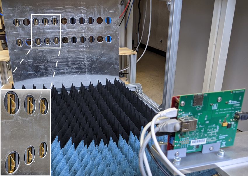
[31], is utilized. The modular front ends were arranged in a As can be observed, the measured value arrives at a minimum
semicircle formation at a distance of Rc = 1 m and behind for ∆τrts = 0.1 ns, which is used to calibrate the RTS channels
a curved metal sheet with round cutouts for the front end for the subsequent measurements. The lateral distance between
antennas. The metal sheet served the purpose of facilitating the two maxima is approximately 1 ns, which is consistent
the positioning of the front ends and the blockage of undesired with (27), as it represents a phase shift of ∆ϕ = 2π. The
radar reflections of the background, leaving only determinable simulation was performed to verify the correctness of the
static reflections. Fig. 3 shows a photo of the measurement preceding analytical derivations. The small difference between
setup. simulation and measurement can be explained by the inaccu-
An UltraScale+ RFSoC FPGA from Xilinx was employed racy, with which the physical positions of the front ends in
for the back end. The integrated ADCs and DACs were config- regards of range and angle were determined by measurement,
ured to a sampling rate of fs = 4 GSPS and the intermediate and to which the simulation was adapted.
frequency was set to frts = 500 MHz. The application of Next, the achievable linearity and its corresponding error
the target’s delay, Doppler shift and attenuation were realized of the synthesized AoA was measured. For this, the required
through sample buffering, a complex quadrature mixer and a delay offset that was determined during the calibration was
linear multiplier, respectively. However, sample buffering at applied to the RTS channels in order to establish phase
the given sample rate only allows for an delay step size of coherency. The angle set-point was linearly increased and the
∆τrts,buf = 0.25 ns, which will later proof to be too coarse for respective signal attenuations were determined according to
the parameter sweep that is necessary for the calibration and (23). Fig. 5 displays the measured and simulated angle value,
This work has been submitted to the IEEE for possible publication. Copyright may be transferred without notice, after which this version may no longer beThis work has been submitted to the IEEE for possible publication. Copyright may be transferred without notice, after which this version may no longer be
accessible.
0
Normalized amplitude
1
0.8
Normalized amplitude in dB
0.6 60 −10
0.4 Front end 1
Range in m
0.2 Front end 2
40 −20
4 5 6 7 8 9 10 11
Set-point angle in deg
(a) Simulated amplitude attenuation 20 −30
Estimated angle in deg
11
0 −40
9 −6 −4 −2 0 2 4 6
Velocity in m/s
7
Simulation Fig. 6: Range-Doppler map of dynamic multi-target
5 Measurement measurement
4 5 6 7 8 9 10 11
Set-point angle in deg 5◦ 0◦ −5◦
10◦ −10◦
15 ◦ −15◦
(b) Simulated and measured angle linearity
60 m
0.2
Angle error in deg
0.1
50 m
Simulation
Measurement
e in m
0
4 5 6 7 8 9 10 11
Rang
Set-point angle in deg
(c) Simulated and measured angle error 40 m
Fig. 5: (a) Amplitude attenuation and
angle (b) linearity and (c) error
TABLE I: Target Characteristics
30 m
Target Range Velocity Angle
1 33.5 m 0 m/s 7° Azimuth angle in deg
2 37 m 4 m/s 4°
3 45 m −2 m/s 10° Fig. 7: Range angle detections of dynamic multi-target
4 52 m −5 m/s 11° measurement
as well as its deviation from its set-points. Measurement and some of which were subject to a Doppler shift. Four targets
simulation both show good agreement between set and actual with characteristics according to Table I were generated by
value, as the maximum angle error of 0.2° correlates to only the RTS simultaneously. Fig. 6 illustrates the range-Doppler
1.14 % in relation to the angle resolution of the RuT. Further- plot measured with a chirp time T = 41.33 µs and with
more, it can be assumed that the angle error occurs due to a Nchirp = 120 chirps. It can be observed, that the targets are
remaining amplitude and phase offset between the utilized RTS generated with the correct range and velocity features. The
channels. The latter could be further reduced by an iterative spurious peaks that occur with an additional range offset to the
calibration with decreasing step sizes for ∆τrts , but can not intended targets are caused by the mismatch of the character-
be eliminated completely as the aforementioned restrictions istic impedance between the front ends and the coaxial cables
still apply. The simulation again serves as a reference for the connected to them. The radar signal travels back and forth
underlying theory developed in the previous chapter. between the back and front end of the RTS, creating ghost
Finally, a measurement was performed with multiple targets, targets with range offsets of multiples of the cable length. The
This work has been submitted to the IEEE for possible publication. Copyright may be transferred without notice, after which this version may no longer beThis work has been submitted to the IEEE for possible publication. Copyright may be transferred without notice, after which this version may no longer be
accessible.
static reflection in close vicinity to the radar can be assigned [12] M. E. Asghar, S. Buddappagari, F. Baumgärtner, S. Graf, F. Kreutz,
to the mechanical structure setup of the RTS. A. Löffler, J. Nagel, T. Reichmann, R. Stephan, and M. A. Hein,
“Radar Target Simulator and Antenna Positioner for Real-Time Over-
Fig. 7 depicts the detected targets in a range-angle map of the-air Stimulation of Automotive Radar Systems,” in Eur. Radar Conf.
the same measurement. All targets are detected at the intended (EuRAD), 2021, pp. 95–98.
angle, demonstrating the suitability of the approach in the [13] S. Graf and M. Rožmann, “OTA radar test for autonomous driving based
on a 77 GHz radar signal simulator,” in Eur. Radar Conf. (EuRAD),
presence of Doppler shifts and underpinning its usability for Workshop: Automot. Radar Meas. Solutions, 2017, pp. 1–19.
scenarios with multiple targets. [14] KEYCOM Corp., “Active Radar Target Simulator for Collision Avoid-
ance Radar (long range),” http://www.keycom.co.jp/eproducts/rat/rat11/
page.html, accessed: 2021-07-01.
V. C ONCLUSION [15] Konrad Technologies, “A Test Solution for ADAS Virtual Test
Drive,” https://www.konrad-technologies.com/en/products/software/
The proposed approach enables radar target simulators to konrad-automotive-radar-test-system.html, 2017, accessed: 2021-07-01.
generate virtual radar targets at an arbitrary angle of arrival. [16] R. Longhurst, Geometrical And Physical Optics. Orient BlackSwan,
The mathematical analysis of the signal model presented 1986.
[17] M. Engelhardt, F. Pfeiffer, and E. Biebl, “A high bandwidth radar target
reveals the constraints that have to be met for a successful simulator for automotive radar sensors,” in Eur. Radar Conf. (EuRAD),
steering of the simulated angle. A calibration method to fulfill 2016, pp. 245–248.
these requirements was developed and simulatively substan- [18] S. Lutz, C. Erhart, T. Walte, and R. Weigel, “Target simulator concept
for chirp modulated 77 GHz automotive radar sensors,” in Eur. Radar
tiated. The approach was implemented on a digital radar Conf. (EuRAD), 2014, pp. 65–68.
target s imulator and the measurement campaign conducted [19] A. Gruber, M. Gadringer, H. Schreiber, D. Amschl, W. Bösch, S. Met-
verifies the practical operation of the calibration procedure zner, and H. Pflügl, “Highly scalable radar target simulator for au-
tonomous driving test beds,” in Eur. Radar Conf. (EuRAD), 2017, pp.
and investigates the achievable linearity of the adjustable angle 147–150.
of arrival. Furthermore, it demonstrates the suitability of the [20] F. Arzur, M. Le Roy, A. Pérennec, G. Tanné, and N. Bordais, “Hybrid
approach for multi target scenarios comprising of non static architecture of a compact, low-cost and gain compensated delay line
switchable from 1 m to 250 m for automotive radar target simulator,”
targets. in Eur. Radar Conf. (EuRAD), 2017, pp. 239–242.
[21] F. Rafieinia and K. Haghighi, “ASGARDI: A Novel Frequency-based
ACKNOWLEDGMENT Automotive Radar Target Simulator,” in IEEE MTT-S Int. Conf. Microw.
Intell. Mobility (ICMIM), 2020, pp. 1–4.
The authors would like to thank PKTEC GmbH for pro- [22] J. Iberle, M. A. Mutschler, P. A. Scharf, and T. Walter, “A Radar Target
viding the front end transceiver hardware and Texas Instru- Simulator for Generating Micro-Doppler-Signatures of Vulnerable Road
Users,” in Eur. Radar Conf. (EuRAD), 2019, pp. 17–20.
ments Inc. for supplying the radar under test. [23] P. Ourednik, A. Zidkov, and P. Hudec, “Doppler Frequency-Shift Unit for
Digital-Analog Automobile Radar Target Simulator,” in Europ. Microw.
R EFERENCES Conf. Central Eur. (EuMCE), 2019, pp. 281–284.
[24] J. Sobotka and J. Novak, “Digital Vehicle Radar Sensor Target Simu-
[1] M. Maurer, J. Gerdes, B. Lenz, and H. Winner, Autonomes Fahren - lation,” in IEEE Int. Instrum. Meas. Technol. Conf. (I2MTC), 2020, pp.
Technische, rechtliche und gesellschaftliche Aspekte. Springer Vieweg, 1–5.
Wiesbaden, 2015. [25] J. Zhang, L. Zhang, P. Gao, and F. Shen, “An FPGA based real-time
[2] S. Schneider, “How to Measure/Calculate Radar System MTBF?” in radar target simulator with high spur suppression,” in 15th IEEE Int.
Europ. Microw. Conf. (EuMC), 2017. Conf. Signal Process. (ICSP), vol. 1, 2020, pp. 126–130.
[3] P. Koopman and M. Wagner, “Challenges in Autonomous Vehicle [26] M. Steins, S. Müller, and A. R. Diewald, “Digital Doppler Effect
Testing and Validation,” SAE Int. Journ. Transp. Safety, pp. 15–24, 2016. Generation with CORDIC Algorithm for Radar Target Simulations,” in
[4] M. Gadringer, H. Schreiber, A. Gruber, M. Vorderderfler, D. Amschl, 23rd Int. Conf. Appl. Electromagn. Com. (ICECOM), 2019, pp. 1–5.
W. Bösch, S. Metzner, H. Pflügl, and M. Paulweber, “Virtual reality for [27] D. Bliss and K. Forsythe, “Multiple-input multiple-output (MIMO) radar
automotive radars,” e & i Elektrotechnik und Informationstechnik, vol. and imaging: degrees of freedom and resolution,” in 37th Asilomar Conf.
135, 06 2018. Signals, Syst. Comput., 2003, pp. 54–59 Vol.1.
[5] J. Iberle, P. Rippl, and T. Walter, “A Near-Range Radar Target Simulator [28] I. N. Bronstein, K. A. Semendjajew, G. Musiol, and H. Mühlig, Taschen-
for Automotive Radar Generating Targets of Vulnerable Road Users,” buch der Mathematik, 5., Ed. Frankfurt am Main: Harri Deutsch, 2001.
IEEE Microw. Wireless Compon. Lett., vol. 30, no. 12, pp. 1213–1216, [29] E. Hecht, Optics, 4., Ed. New York: Pearson, 2012.
2020. [30] S. Scherr, “FMCW-radarsignalverarbeitung zur entfernungsmessung mit
[6] S. Wald, T. Mathy, S. Nair, C. M. Leon, and T. Dallmann, “ATRIUM: hoher genauigkeit,” Ph.D. dissertation, Karlsruhe, 2017.
Test Environment for Automotive Radars,” in IEEE MTT-S Int. Conf. [31] A. Diewald, C. Kurz, P. V. Kannan, M. Gießler, M. Pauli, B. Göttel,
Microw. Intell. Mobility (ICMIM), 2020, pp. 1–4. T. Kayser, F. Gauterin, and T. Zwick, “Radar Target Simulation for
[7] M. E. Gadringer, F. M. Maier, H. Schreiber, V. P. Makkapati, A. Gru- Vehicle-in-the-Loop Testing,” Vehicles, vol. 3, no. 2, pp. 257–271, 2021.
ber, M. Vorderderfler, D. Amschl, S. Metzner, H. Pflügl, W. Bösch,
M. Horn, and M. Paulweber, “Radar target stimulation for automotive
applications,” IET Radar, Sonar Navigat., vol. 12, no. 10, pp. 1096–
1103, 2018.
[8] M. Steins and A. R. Diewald, “Implementation of delay line with fine
range discretization for radar target simulations,” in 19th Int. Radar
Symp. (IRS), 2018, pp. 1–9. Axel Diewald (GS’18) received the B.Sc. and M.Sc.
[9] G. Körner, M. Hoffmann, S. Neidhardt, M. Beer, C. Carlowitz, and degrees in electrical engineering and information
M. Vossiek, “Multirate Universal Radar Target Simulator for an Accurate technology from Karlsruhe Institute of Technology
Moving Target Simulation,” IEEE Trans. Microw. Theory Techn., vol. 69, (KIT) in Karlsruhe, Germany, in 2015 and 2017
no. 5, pp. 2730–2740, 2021. respectively. Since 2018, he is pursuing a doctorate
[10] A. Diewald, T. Antes, B. Nuss, and T. Zwick, “Implementation of Range (Ph.D.E.E.) degree at the Institute of Radio Fre-
Doppler Migration Synthesis for Radar Target Simulation,” in IEEE 93rd quency Engineering and Electronics (IHE) at the
Veh. Technol. Conf. (VTC2021-Spring), 2021, pp. 1–5. KIT. His main fields of research interest are digital
[11] Rohde & Schwarz, “R&S AREG800A: Automotive Radar Echo radar target simulation for the purpose of automotive
Generator,” https://scdn.rohde-schwarz.com/ur/pws/dl downloads/dl radar sensor validation as well as realistic target
common library/dl brochures and datasheets/pdf 1/AREG800A bro modeling.
en 3609-8015-12 v0100.pdf, 2021, accessed: 2021-07-01.
This work has been submitted to the IEEE for possible publication. Copyright may be transferred without notice, after which this version may no longer beThis work has been submitted to the IEEE for possible publication. Copyright may be transferred without notice, after which this version may no longer be
accessible.
Benjamin Nuss (GS’16) received the B.Sc. and
M.Sc. degrees in electrical engineering and infor-
mation technology from the Karlsruhe Institute of
Technology (KIT), Karlsruhe, Germany, in 2012
and 2015, respectively, where he is currently pur-
suing the Ph.D. degree in electrical engineering at
the Institute of Radio Frequency Engineering and
Electronics (IHE). His current research interests
include orthogonal frequency-division multiplexing-
based multiple-input multiple-output radar systems
for future automotive applications and drone detec-
tion. The focus of his work is the development of efficient future waveforms
and interference mitigation techniques for multiuser scenarios.
Mario Pauli (S’04–M’10–SM’19) received the
Dipl.Ing. (M.S.E.E.) degree in electrical engineering
and Dr.-Ing. (Ph.D.E.E.) from the University of
Karlsruhe, Karlsruhe, Germany, in 2003 and 2011,
respectively.
Since 2011 he is with the Institute of Radio Fre-
quency Engineering and Electronics at the Karlsruhe
Institute of Technology (KIT) as a Senior Researcher
and Lecturer. He served as a Lecturer for radar and
smart antennas of the Carl Cranz Series for Scientific
Education. He is co-founder and the Managing Di-
rector of the PKTEC GmbH. His current research interests include radar and
sensor systems, RCS measurements, antennas and millimeter-wave packaging.
Thomas Zwick (S’95–M’00–SM’06–F’18) re-
ceived the Dipl.-Ing. (M.S.E.E.) and the Dr.-Ing.
(Ph.D.E.E.) degrees from the Universität Karlsruhe
(TH), Germany, in 1994 and 1999, respectively.
From 1994 to 2001 he was a research assistant at the
Institut für Höchstfrequenztechnik und Elektronik
(IHE) at the Universität Karlsruhe (TH), Germany.
In February 2001, he joined IBM as research staff
member at the IBM T. J. Watson Research Center,
Yorktown Heights, NY, USA. From October 2004 to
September 2007, Thomas Zwick was with Siemens
AG, Lindau, Germany. During this period, he managed the RF development
team for automotive radars. In October 2007, he became a full professor at
the Karlsruhe Institute of Technology (KIT), Germany. He is the director of
the Institute of Radio Frequency Engineering and Electronics (IHE) at the
KIT.
Thomas Zwick is co-editor of 3 books, author or co-author of 120 journal
papers, over 400 contributions at international conferences and 15 granted
patents. His research topics include wave propagation, stochastic channel mod-
eling, channel measurement techniques, material measurements, microwave
techniques, millimeter wave antenna design, wireless communication and
radar system design.
Thomas Zwick’s research team received over 10 best paper awards on
international conferences. He served on the technical program committees
(TPC) of several scientific conferences. In 2013 Dr. Zwick was general chair of
the international Workshop on Antenna Technology (iWAT 2013) in Karlsruhe
and in 2015 of the IEEE MTT-S International Conference on Microwaves for
Intelligent Mobility (ICMIM) in Heidelberg. He also was TPC chair of the
European Microwave Conference (EuMC) 2013 and General TPC Chair of
the European Microwave Week (EuMW) 2017. In 2023 he will be General
Chair of EuMW in Berlin. From 2008 until 2015 he has been president of
the Institute for Microwaves and Antennas (IMA). T. Zwick became selected
as a distinguished IEEE microwave lecturer for the 2013 to 2015 period
with his lecture on “QFN Based Packaging Concepts for Millimeter-Wave
Transceivers”. Since 2017 he is member of the Heidelberg Academy of
Sciences and Humanities. In 2018 Thomas Zwick became appointed IEEE
Fellow. In 2019 he became the Editor in Chief of the IEEE Microwave and
Wireless Components Letters. Since 2019 he is a member of acatech (German
National Academy of Science and Engineering).
This work has been submitted to the IEEE for possible publication. Copyright may be transferred without notice, after which this version may no longer beYou can also read