ASIRI Boundary layers in the Bay of Bengal - Amit Tandon UMass Dartmouth - KITP Online Talks
←
→
Page content transcription
If your browser does not render page correctly, please read the page content below
Boundary layers in the Bay of Bengal
                         Amit Tandon                 ASIRI
                       UMass Dartmouth

                                   Summer
                                 Monsoon winds

                       Arabian              Bay of
                        Sea                 Bengal

                                 Northern
                                  Indian
earth.nullschool.net              Ocean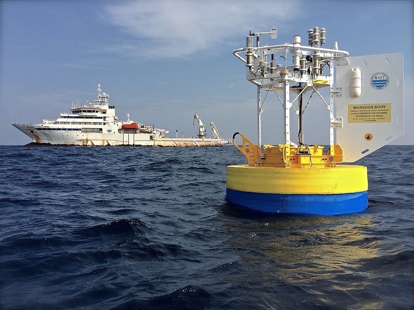
2.5 billion people depend on the Monsoon for water, food, economy

                                                            Bay of Bengal

                                                            •   Highest per
                                                                capita
                                                                impact of
                                                                oceanic
                                                                influence
                                                            •   Largest
                                                                human
     World Population as a function of Longitude   Bay of       susceptibility
                                                   Bengal       to climate
                                                                change.
                       Atlantic
Motivation for ASIRI
•   Almost a third of the world’s population depends on the
    South Asian Monsoon for water
•   Climate models have difficulty in predicting the monsoons,
    particularly their sub-seasonal variability (active/break
    periods).
•   The ocean supplies heat and moisture for the monsoon.
    Role of oceans is important, but in coupled models SST is
    too cold.
•   Upper ocean structure, physical processes, and air-sea
    interaction affect the SST.
•   The Bay of Bengal is strongly affected by freshwater from
    the monsoons. How does this modify oceanic processes?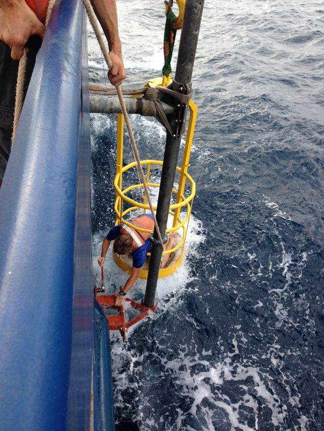
While forecast skill for precipitation is good for El-Nino
         region, it is very poor for the Asia-Western Pacific!

            El Nino region (10oS-5oN, 80oW-180oW)
                  WNP (5-30oN, 110-150oE)
            Asian-Pacific MNS (5-30oN, 70-150oE)
                                                                         Area averaged correlation coefficient
Correlation Coefficient between the observed and Multi-Model-Ensemble   between model and observations (skill)
                  hindcasted June-August precipitation

                                                     (Bin Wang, et al. 2005)

 ➡    Coupling of upper ocean with lower atmosphere is key to better
                prediction of tropical storms in this region.
 ➡      ONR motivation: Safety of ships at Sea, Active-Break periods
                   of the Monsoon impact wave forecasts
 ➡       India MoES motivation: Better characterization of air-sea
           interaction is important to improve Monsoon forecasts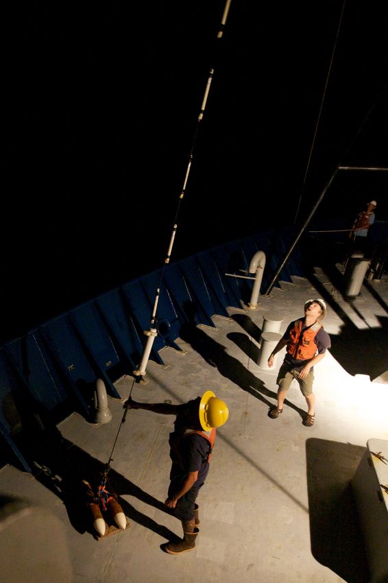
Monsoons: A challenge for prediction
                      Active & break periods
                                                                      Goswami (2016)              1986
                                                                                                 drought
                                                                                                   year

          Why Bay of Bengal?
                                               Genesis and tracks of depressions
                                                                            Goswami (2016)
            Why North Bay?

Weakness of coupled forecast
                                                     Ocean: What is affecting the monsoon forecasts?
models                                               (1) Poorly known air-sea fluxes in the Bay.
•   Ocean is poorly represented                      (2) Unique ocean response, mixing and boundary
•   Sea surface too cool, stratification weak        layer physics in the region is not well understood and
                                                     not captured by GCMs.
•   Intra-seasonal variability not captured          (Collection of papers by IITM Pune 2016)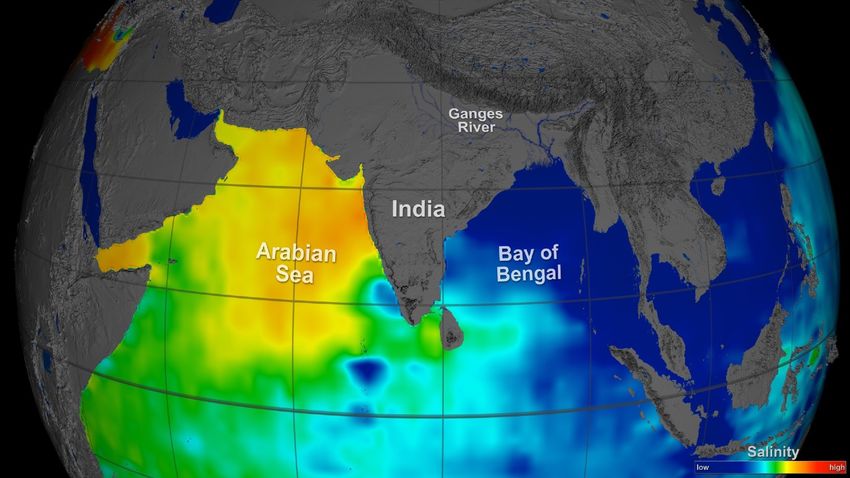
Monsoon rainfall

Bay of Bengal: An unusually fresh ocean

                     Sea surface salinity
                      Aquarius satellite
                           (Oct)

                                                Bay of Bengal

                                            Salinity: NRL Model
Bay of Bengal - anomalous ocean
• Winds & Circulation reverse seasonally                    India       Mahanadi
                                                                                   Ganges-Brahmaputra

• Extremely fresh
                                                                                                        Irrawaddy
                                                            Godavari

                                                             Krishna

                                              Arabian Sea              Bay of Bengal

• Highly stratified, poorly ventilated
• Warm surface - SST responds quickly
• Air-sea fluxes ! FW runoff
• Oxygen minimum zone
                                      Surface salinity from the Aquarius satellite, Fall 2013

                                                                Monsoon ISV - “active-break” cycle
                                               Salinity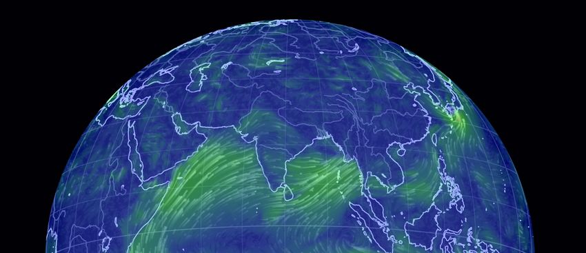
What sort of program ?
                       Toward improving the monsoonal forecast
                                                                                           ASIRI
                                       Modeling and Prediction
                                            Coupled models
                                             Assimilation
                                                                                    MISOBOB

Data for model testing and              Improve representation of             Parameterize processes
       improvement                          Boundary layers                        and fluxes
                                             Air-sea fluxes
                                           Subgrid processes
             Observations                                                Process Studies
          Mooring, floats, gliders,                                      Multi-scale modeling
          drifters, ships, satellite                                     Process experiments

      Measurements - upper ocean                                    Understand physical processes,
      structure, fluxes, phenomena                                  explore parameter dependence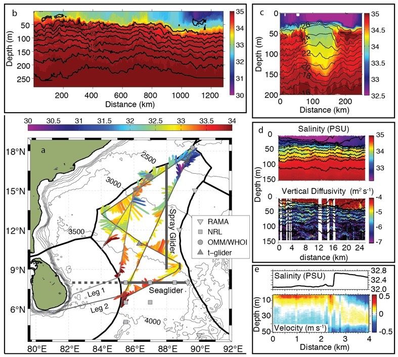
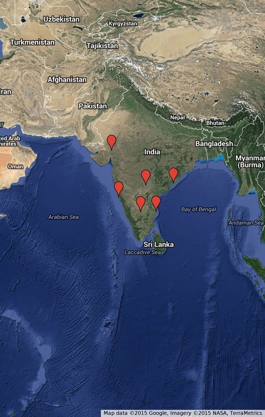
10 USA Institutions (about 20+ US PIs) and 8 Indian
    institutions (10+ Indian PIs) collaborating

              SAC,ISRO#Ahmedabad#

                                 INCOIS#and#TIFR#Hyderabad#

                                                   IIT#Bhubaneswar#
                  NIO#Goa#                     NIO#Vishakapatnam#

                                           NIOT#Chennai#and#IIT#Madras#

                             IISc#Bangalore#

                                           EBOB#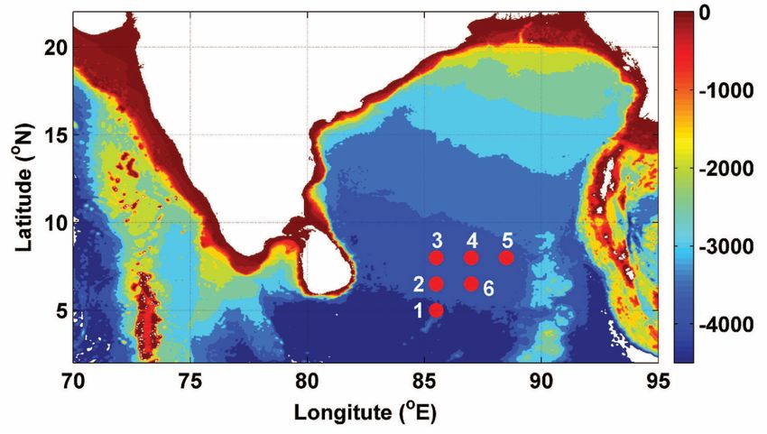
ASIRI – OMM: Observations Begin!                               ASIRI

• Nov-Dec 2013.
  – Survey and Process Experiment 1: R/V Revelle with US and Indian
    teams; Cruise on Nidhi with Indian and US scientists

• 2014:
  – Survey and Process Experiment 2: Pre-Monsoon observations with
    Indian scientists in international waters (June, R/V Revelle Chennai
    Port call)
  – July: Summer Workshop on Upper Ocean Physics in the Bay of
    Bengal; August 2014.
  – August: R/V Nidhi Monsoon cruise with Indian and US scientists
  – Nov.-Dec.: Flux mooring deployment from R/V Nidhi

• August-September 2015. Survey and Process Experiment 3: SW
  Monsoon Intensive Observational Period on US R/V Revelle and Indian
  ships.
ASIRI: OBJECTIVES What is the role of freshwater and seasonality of forcing on the upper ocean structure and circulation of the Bay of Bengal? 1. Boundary forcing: What is the variability in air-sea flux and boundary inputs? How are they affected by (and affect) freshwater distribution? Will accurate boundary fluxes improve forecasting of upper ocean structure and evolution? 2. How are physical processes, such as 1-d wind-driven mixing, Ekman transport, mesoscale circulation (nominally already included in models) playing out in unusual ways here? 3. What sets the stratification (submesoscale mixing and/or re-stratification, episodic events like strong cyclones, internal wave breaking, or others) ?
ASIRI: OBJECTIVES - 1

            Boundary forcing: What is the
            variability in air-sea flux and
            boundary inputs? How are they
            affected by (and affect)
            freshwater distribution? Will
            accurate boundary fluxes
            improve forecasting of upper
            ocean structure and evolution?
Need for benchmark measurements
of air-sea fluxes
Lack of agreement in air-sea fluxes from
different reanalysis products.JJA AVISO
Wind- ASIRI: OBJECTIVES - 2 SSH
SST (MAM)
How are physical processes, such as 1-d wind-driven mixing,
Model – Buoytransport,
Ekman SST/SSS Temporal Change
mesoscale circulation (nominally
Modelalready
– Satellite Comparison
18 N 89.5 E : (OMM-Mooring)
included in models) playing out in unusual ways here?
GHRSST Model
JJA SSH
Wind- AVISO
Winds
SSS SSH (JJA)
e Winter Model – Satellite Comparison
GHRSST SST Model Surface Salinity
Strong Coupling SMAP
Is the air-sea coupling linked to the weak/strong eddy Model
Salinity gradients areactivity???
weak in model
ASIRI-OMM Science Meeting: 9-10 Jan, 2017
Sarma et al.Observational Focus- Mapping the full-scale of
Physical Processes at work in the Bay of Bengal
Instrumental &
Observational
Challenge
Our approach
integrating moored
time series,
autonomous
assets, &
shipboard surveys
with state of the art
instrumentationASIRI: OBJECTIVES - 3
T
What sets the
Salinity along transect
stratification
(submesoscale mixing
and/or re-stratification,
S
episodic events like 13
strong cyclones,
internal wave
breaking, or others) ?
N2
Distance along trackASIRI
Science Results: What we have learned?
What improvements are possible for weather
and ocean forecasting?
A. Large pools of sub-surface warm water in Barrier layers.
B. Microstructure and scalar mixing in the BoB.
C. What air-sea flux variations prediction models are missing - and why.
D. Interplay of mesoscale eddies, wind and the freshwater from rivers
sets the multiple stratification layers.
E. Unprecedented near-surface process observations near frontsASIRI 2013-2017:
Outcomes
with International Collaboration in the
region
MISO-BOB 2017-2021
• Air-sea flux measurements + solar input
Long term observatory • Test bulk formulae, improve models
• Upper ocean vertical structure
• Relate to air-sea fluxes and stratification
Measure mixing rates • Test and improve parameterizations
• Improve upper ocean structure in models
• Understand freshwater dispersal mechanisms
Process modeling • Understand mixing processes
• Estimate advection - test for seasonal variationsCentral
J O U Bay Process
RNAL O F P H Y S I C A LStudy:
O C E A N O GNov,
R A P H Y 2013 Aquarius
VOLUME 48 salinity
+
CCAR SSHA
Mesoscale strain
(OSCAR) ~ 0.15 f
0-10 m averaged
potential density
UCTD resolution: 0.7-1.0 km
Duration of transects: 4-6 hrs
Ramachandran, Tandon et al. March 2018 JPO
FIG. 1. CCAR SSHA (color) for the week starting 18 Nov 2013 and salinity contours (black
21
solid and dashed; g kg ) for the week starting 12 Nov 2013 from the level 3.0 AquariusRamachandran, Tandon et al. March 2018 JPO
ADCP Lucas
Pinkel
Waterhouse
Wirewalker
Analysis Tandon
Mackinnon
Ramachandran Shroyer
UCTD
Weller
Met. data
Nash Farrar
Mahadevan• StandardMeasurements
shipboard throughflow T&Sused ! in this study
• Underway CTD!
• Underway CTD
• Thermistor+CTD bow-chain!
• Wirewalker
• Spar buoy: freely drifting, upward looking
• ADCPs
Standard shipboard
at 20 and through flow T & S
xx meters below
surface, regularly spaced thermistors !
• Shipboard met.
data
•• Hull-mounted
Permanent sonars
ADCPs on the ship (4)
+ HDSS!
• Side-pole
• Side-pole mounted ADCP
ADCP + Pipestring ADCPSurface Forcing
JOURNAL OF PHYSICAL OCEANOGRAPHY VOLUME 4
22T and S sections for each
MARCH 2018 R A M A of
CHAthe
NDRtransects
AN ET AL. 485
21Pycnostads
Transect BLarge ⇣ ⇡ @v/@x
Transect B⇣/f ⇡ 35
Transect CVorticity is O(f) with more structure emerging as scales get finer.
Positively skewed
JOURNAL OF PHYSICAL OCEANOGRAPHY VOLUME 48
FIG. 6. Vertical vorticity, z ’ ›y/›x, scaled with the Coriolis parameter, for transect C, s
(a) 2 km, (b) 4 km, (c) 8 km, and (d) 16 km. The color bar on top is for (a) and (b) while that
The solid lines are isopycnals obtained from the UCTD measurements, spaced 0.05 kg m2
the same scale as the vorticity field in each panel. (e) Skewness of z ’ ›y/›x at 8-km scale, ob
from the five transects at each depth.
Transect C
as follows. Along each transect, we first locate the po- frontal axis consistently, we
Are these fronts in balance?
sition where the magnitude of the lateral buoyancy fronts closer to the northe
gradient at the surface is maximum (Johnston et al. The locations of the fronta
2011). This procedure yields a location that alternates A to E, xFR 5 (28, 28, 28Geostrophy
For a linear regression model:
ig
ez = a
u r⇢
f ⇢0
the smallest residual occurs when
if ⇢0 huz r⇢⇤ i
a=
g hr⇢r⇢⇤ i
For thermal-wind balance, a=1
Rudnick and Luyten (1996)Low-pass: 8 km
• What types of submesoscale
instabilities is this weakly
geostrophic flow unstable to?Cooling
Winds Frontogenesis
PV < 0
Subduction
Creation of zero
PV by SI, inertial
instability
Transect BPV forcing and budget
pt for a portion of 1 ›b ›b
EBF 5 ty 2 tx . (7)
dix B), where the r0 f ›x ›y
ccur during
492 a pe- JOURNAL OF PHYSICAL OCEANOGRAPHY VOLUME 48
The gradients in Equation (7) shows winds with a downfront component
ignificant in this result in a positive EBF and thus extract PV from the
B). surface. In using (7), we neglect the term containing
r-zero or negative ›b/›y (justification in appendix B). The EBF is also some-
ral extent of these times expressed as an Ekman heat flux (W m22; Fig. 2b)
respectively. The EHF 5 [r0Cp/(ag)]EBF, where a is the thermal expan-
y low’’ or ‘‘vorti- sion coefficient for seawater and Cp 5 3984 J kg21 8C21 is
results principally the specific heat of seawater at constant pressure (Thomas
, resulting in low q 2005). In using (5), we replace z with f as we lack in-
1 f is the absolute formation about the vorticity field at the surface. Evalu-
w PV are seen in ating (5) with z at z 5 28 m reduces slightly the injection
with PV , 0, lo- of PV into the mixed layer during transects C and D. For
sopycnals (Fig. 8), the other transects, the rate of PV extraction is virtually
hese contrast the indistinguishable from that obtained by setting z 5 f in (5).
sitive, q and weak Integrating (4) vertically over the mixed layer,
absence of strong FIG. 9. (a) Ertel PV averaged over the mixed layer corresponding to an increment of
ð $
Dr 5 0.2 kg m23 from 0a depth of 1 m. (b) Net buoyancy flux at the ocean0 surface (W kg21; line
ve z. › 1 ›q 1 $ 1
hqi 5 H
5 2 (J DIAB fromFRIC
with circles), Ekman buoyancy flux (W kg21) obtained
z 1J z )$$ 2
15-min winds and the buoyancy
( . . . ),
›t H 2H ›t H H
field at a depth of 1 m, smoothed to 8 km. A positive flux indicates cooling of the ocean.
2H averaged over the
surface fluxes (c) Contribution (s24) from the diabatic and frictional flux to the PV budget
mixed layer. (8)
PV q is governed
The
Nmchanges
r J (Marshall and in PV are
is the bulk stratification
where h!i H
large,
between
denotesand
1 m and
DIAB
the cannot
mixed allbe
averaging
FRIC
five explained
over byestimates
transects. These
H. The surface
parentheses forcing.
describe These changes
averages
layer depth. The combined effect of Jz and Jz is between the mixed layer base and 8 m. The magni-
happen over
mostly to extractinPV,a longer
theexcept time
finalwhen
term scale than
solaronheating, the side
the right
tudes survey
range of (advected
from (8)
O(10represent
210 into
) s23 (for A, the sampled
B, and D) to volume)
through JzDIAB , injects PV into the mixed layer (Fig. 9c). O(10 29 ) s 23 (for C and E). Thus, the lateral advective
Integrating 2(JzDIAB 1 JzFRIC )/H over the duration of flux, as approximated here, is also incapable of gener-
transect A yields 27.57 3 10210 s23, the PV extracted ating O(1028) s23 variations in hqiH over the duration
from the mixed layer. Bulk of the PV removal (69%) of a transect.Potential instabilities when f q < 0
Thomas et al. (DSR, 2013)
✓ ◆ ✓ 2
◆
1 (⇣ + f ) 1 |rh b|
c = tan RiB = tan
f f 2N 2Inertial
instability
Stable Unstable
Symmetric
instability
Cushman-Roisin and BeckersVortically low
Baroclinically low
Where is the flow unstable?
Ertel PV at
Unstable to FSI
8 km scaleNormalized PV and balanced Ri = f2N2/M4
JOURNAL OF PHYSICAL OCEANOGRAPHY VOLUM
The presence of these regions
with flow conditions close to
neutral stability for FSI (Ri
slightly larger than unity) in the
vicinity of other regions where
FSI might be active, is
suggestive of the neutrally
stable Ri resulting from earlier
FSI events.Transect A @Mabs /@x ⇥ 103 (8 km scale)
SI
SI + Inertial instability
Lateral extent of alignment in
agreement with length scale for
most unstable hydrostatic SI
mode
Symmetric instability:
Alignment of contours of
Mabs = v + f x Mabs and density (2 km scale)
@Mabs /@x < 0 =) Inertial instability
Contours are absolute momentum
Color: Gradient of absolute momentum (8km fields)Confluent flow
Isentropic PV
f + ⇣⇢ ⇢
PV⇢ =
P ⇢
@v
⇣⇢ ⇡
@x ⇢
We would like to see the
imprint of lateral velocity
gradients in the spatial
variability of N2
Pollard and Regier (1992).regions of
constant IPV
where the
thickness
between
isopycnals
and vorticity
on density
surface
mutually
compensate
each other
t = 20.7
t = 20.8
t = 20.9
t = 21Cooling
Winds Frontogenesis
PV < 0
Subduction
Creation of zero
PV by SI, inertial
instability
Transect BSummary Fronts in the northern Bay are sharp, shallow and stratified. Observations at a salinity front forced with downfront winds and moderate mesoscale frontogenesis show a range of submesoscale processes at play • Negative Ertel PV, O(f) vorticity • Symmetric instability, inertial instability Below the top 10 m, isopycnal thickness and isentropic vorticity vary in lockstep • Pycnostads with O(1-10 km) lateral scales. Similar dynamical markers missing at a second process study in winter forced by upfront winds and weak frontogenesis. 2015 data analysis shows intriguing results (ongoing)
Ertel PV     Was CBPS special?

    Upfront winds and weak strain at   17.3N
You can also read