Assessing the adverse effects of a mixture of AMD and sewage effluent on a sub tropical dam situated in a nature conservation area using a ...
←
→
Page content transcription
If your browser does not render page correctly, please read the page content below
International Journal of Environmental Research (2021) 15:321–333
https://doi.org/10.1007/s41742-021-00315-3
RESEARCH PAPER
Assessing the adverse effects of a mixture of AMD and sewage effluent
on a sub‑tropical dam situated in a nature conservation area using
a modified pollution index
Petrus F. Oberholster1 · Jaqueline Goldin1 · Yongxin Xu1 · Thokozani Kanyerere1 · Paul J. Oberholster1,2 ·
Anna‑Maria Botha3
Received: 10 September 2020 / Revised: 17 December 2020 / Accepted: 18 January 2021 / Published online: 19 February 2021
© University of Tehran 2021
Abstract
Currently water resources in nature conservation areas are under severe pressure due to external drivers of anthropogenic
pollution. There is a lack of monitoring tools to determine water quality status of dams situated in nature reserves receiv-
ing a mixture of pollutants over space and time. The present study was conducted over a 12-month period with the aim of
applying a modified pollution index (PILD) to determine the water quality and phytoplankton status of the Loskop Dam
situated in the Loskop nature reserve, South Africa. From the data generated in the current study, it was evident that the
PILD effectively determined nutrient enrichment and heavy metal pollution in the dam. Furthermore, the study showed that
the most pollution tolerant phytoplankton species was the diatom Melosira varians followed by the dinoflagellate Ceratuim
hirundinella and the cyanobacteria Microcystis aeruginosa. Chemical variables during the sampling period that exceeded
the limits of the South African, Canadian, Australia and New Zealand guideline levels were Zn, TP, Cl, Fe, Mn and N H 4.
The occurrence of concentrations of Cl above the target water quality range for aquatic ecosystems (5 µgl−1) over the entire
sampling period, may have been related to point source sewage pollution in the upper catchment. The PILD showed poor
water quality conditions during the months of September and October during the dam’s destratification (lake overturn). By
modifying an existing index to incorporate physico-chemical variables that are strongly related to a mixture of pollutants, it
should have application on global scale applied to different waterbodies with differ phytoplankton indicator species across
different geographical regions. Furthermore, it could also in the future serve as a decision support tool for conservation
managers to determine the pollution status of a dam situated in nature conservation areas receiving a mixture of pollutants.
* Anna‑Maria Botha
ambo@sun.ac.za
1
Department of Earth Sciences, Faculty of Natural Sciences,
University of the Western Cape, Private Bag X17,
Bellville 7535, South Africa
2
Centre for Environmental Management, University
of the Free State, Private Bag 339, Bloemfontein 9300,
South Africa
3
Genetics Department, Stellenbosch University, Private Bag
X1, Matieland, Stellenbosch 7601, South Africa
13
Vol.:(0123456789)322 International Journal of Environmental Research (2021) 15:321–333
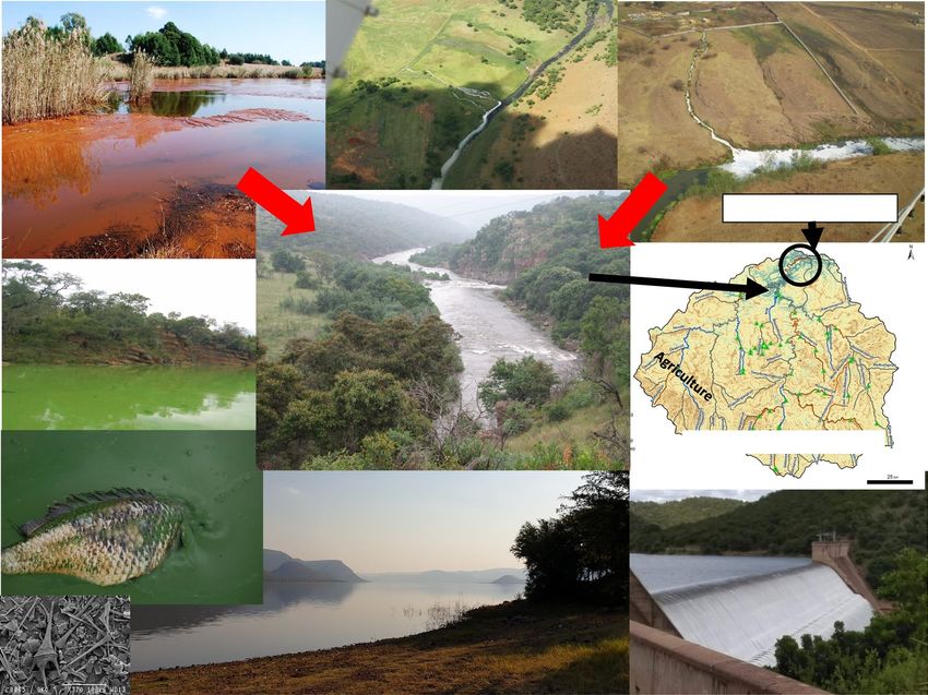
Graphic abstract
Inflow of sewage from
dysfunc
onal WWTPs up-steam in
the river catchment
Acid mine drainage
inflows because of
mining ac
vity
Loca
on of Loskop Dam
Olifants River gorge
High density coal mining
Cyanobacterial
blooms and fish Upper catchment of the Olifants River
mortali
es
Loskop Dam, South Africa
located within a nature
reserve
Ceraum sp.
Keywords Conservation area · Mixture of pollutants · Modified pollution index · Phytoplankton
Introduction Land use in the catchment is dominated by extensive coal
mining in the Witbank Coalfields, which are located in the
Over the past two decades, isolated incidents of mass fish headwaters of the Olifants River, upstream of Loskop Dam
mortality have been recorded at different times in Loskop causing Acid Mine Drainage (AMD) (Oberholster et al.
Dam, South Africa. These incidents have become more fre- 2017; Lebepe et al. 2020). Heavy metals from the latter can
quent during 2003–2008 (Dabrowski et al. 2013) and coin- be a risk to the eco-environment and human health (Kumar
cided with Nile crocodile (Crocodylus niloticus) and terrapin et al. 2020a, 2020c). With the latter background in mind, we
(Pelomedusa subrufa) mortalities. The crocodile population proposed to develop a pollution index that can assist con-
in Loskop Dam has declined from approximately 30 animals servation managers globally to monitor polluted dams in
to a total of 6 in 2008 (Dabrowski et al. 2013). Crocodile conservation areas using Loskop Dam as a case study.
mortality in Loskop Dam during this time was ascribed to Numerous biological assessment tools have been devel-
pansteatitis, which is associated with the intake of rancid oped globally for different types of aquatic ecosystems and
fish fat after a fish die-off. During 2008, the crocodile popu- for various monitoring purposes (Bain et al. 2000; Simon
lation in the Olifant’s River Gorge downstream of Loskop 2000; Kumar et al. 2020b). Making use of bio-indicators,
Dam in the Kruger National Park, which is one of the largest species may prove an accurate description of the status and
conservation areas in Africa, declined from 1000 to 400. cumulative deterioration of an aquatic ecosystem (Castro-
Furthermore, Loskop Dam also showed signs of eutrophi- Roa and Pinilla-Agudelo 2014). Phytoplankton are of key
cation conditions over the last two decades with large toxic ecological importance because of the major role they play
cyanobacterial blooms occurring sporadically (Oberholster in aquatic food web interactions. Phytoplankton communi-
et al. 2010; Dabrowski 2014). ties are extremely dynamic and respond to changes in light,
nutrients and sediment loads, rapidly changing in biomass
13International Journal of Environmental Research (2021) 15:321–333 323
distribution and species composition; thereby, making them of bio-indicators, but the index only focusses on a selected
good indicators of aquatic health and water quality (Castro- group of species which only indicates organic pollution. In
Roa and Pinilla-Agudelo 2014). a complex aquatic system where different sources of con-
Currently, there is an urgent need to generate instruments tamination (i.e., mixture of AMD and sewage effluent) are
(e.g., monitoring indices) that can help to preserve threat- present, it is important to select the best index or to modify
ened aquatic ecosystems in nature reserves and to identify an existing index to generate the best results.
and prevent the contamination of watersheds. The following Although not much is known about the mixture of AMD
characteristics are important indicators of a good index: (1) and sewage effluent under reservoir conditions, the treatment
The index must focus both on physico-chemical parameters of AMD by municipal wastewater is a well-documented
and biological indicators. Biological and chemical indica- principle (Roetman 1932; McCullough et al. 2008). An ear-
tors all provide information about a waterbody. A biologi- lier study by McCullough and Lund (2011) investigated the
cal index, in the absence of other supporting information, treatment of AMD using sewage and green yard waste as
can provide significant insight into the degree of stress to organic source to reduce sulphate concentrations in micro-
which a waterbody is subjected. (2) The index can be applied cosm experiments, containing pit lake water with a pH of
to study a complex aquatic ecosystem by giving biologi- 2.4. The authors found higher bioremediation rates in AMD
cal communities each a single numerical value to indicate treated with sewage than green yard waste. In multi-stage
their resilience towards contamination. A common occurring studies of co-treatment of synthetic AMD and municipal
problem with most indices, for example that of Kothe’s, is wastewater conducted by Strosnider et al. (2011a; b), the
that it only takes into account the response of a single taxon authors reported the decrease in Al, As, Cd, Fe, Mn, Pb
to assess the condition of a sample site, which could include and Zn by 99.8%, 87.8%, 97.7%, 99.8%, 13.9%, 87.9% and
“suspect” species that can tolerate pollution. (3) Most of the 73.4%, respectively, with a net acidic influent conversion
indices that has been developed for biological monitoring to net alkaline circumneutral effluent. The system received
focused only on river organisms. This meant that the pollu- municipal wastewater with a mean BOD5 of 265 mgl−1 and
tion index might not provide informative data for assessment produced effluent with a BOD5 below detection limit.
if applied to a stationary water body such as lakes, dams and The objectives of the current study were: (1) to apply
ponds. Therefore, a good pollution index must be flexible so a modified pollution index to determine the status of the
that it can be modified to assess different types of waterbod- water quality of a dam situated in a nature reserve receiving
ies, as well as using different indicator species. a mixture of AMD and sewage effluent, and (2) to determine
The pollution index developed by Jiang and Shen (2003) if this index tool can be used as a decision support tool for
for example, was first used to assess protozoan communities conservation managers by identifying changes in waterbody
in the River Hanjiang, China. The method was then modi- water quality over space and time.
fied by Costro-Roa and Pinilla-Agudelo (2014) to assess the
condition of five wetlands in Bogotá and one rural wetland
(Brazilia) during which they used diatoms as indicators of Materials and methods
pollution. (4) Most indices make use of limited data sets.
When using this method there is flexibility in the type of Study area
data that can be collected and combined. In the studies of
Kumar et al. (2020a and b) more than one method was uti- South Africa possesses approximately five percent of the
lised to provide a better assessment. As previously stated, global recoverable coal reserves and is also the world’s sixth
most indices only focus on one specific aspect to assess largest coal producer. The Witbank coalfields, in Mpuma-
aquatic pollution, so more than one pollution index needs to langa Province, South Africa, represent the largest area of
be implemented to have a greater understanding on the level active coal mining in the country and are located in the Olif-
of pollution (Mishra et al. 2016). When utilising the chosen ants River catchment, resulting in the river being considered
method, the assessment is more comprehensive as it incor- to be one of the most polluted rivers in southern Africa (Leb-
porates both the biological organisms that act as “indicators” epe et al. 2020). Mining activity causes mine dewatering
of pollution and the national and international standards to which results in a discharge of approximately 50 Ml per day
assess physico-chemical contamination. (5) The index must of mine water into the upper Olifants River catchment (Dab-
have the ability to make use of any organisms as “bio-indica- rowski et al. 2014). Other land use activities in the upper
tors”. According to Bellington et al. (2010) most of the other catchment that have major impacts on water resources are
indices utilising bio-indicators only use diatoms, such as the effluent from wastewater treatment plants (WWTPs). Thirty-
indices of Sládeček (1986) and Kelly and Whitton (1995). two of the WWTPs are not operated optimally according to
This means that these only focus on one specific group of the National Green Drop (GD) Report of 2010 (DWA 2010;
organisms. Palmer’s index (1969) for example makes use Oberholster et al. 2013). It was evident from this National
13324 International Journal of Environmental Research (2021) 15:321–333
Green Drop report that most of the WWTP’s in the upper three subsamples of 2 L each for the following analyses: (a)
catchment had an overall score of less than 30%, showing Two litres were filtered through 0.45 µm pore size Whatman
that many of these plants are in a critical, dysfunctional GF/filters for dissolved nutrient analyses; (b) Two litres were
state. In a previous study by Oberholster et al. (2017) the filtered through 1 µm Gelman glassfibre filters and preserved
authors demonstrated that although neutralization of AMD in nitric acid for metal analyses; and (c) Two litres was pre-
and acid precipitation by sewage effluent were evident in the served in the field by addition of acidic Lugol’s solution to
upper Olifants River catchment, the deterioration in environ- a final concentration of 0.7%, followed after one hour by the
mental conditions and associated shifts in biological com- addition of buffered formaldehyde to a final concentration
munities were distinct. In the upper Olifants catchment, the of 2.5% for phytoplankton identification. All sampled water
Loskop Dam (25º 26′ 57. 05" S; 29º 19′ 44. 36 E) acts as a was stored in polyethylene bottles that had been pre-rinsed
repository for these pollutants and was selected as current with dilute sulphuric acid (to pH 2.0). The Standard Meth-
case study (Grobler 1994) (Fig. 1). The sub-tropical dam is ods for the Examination of Water and Wastewater (APHA
surrounded by 23 612 ha of nature reserve and contains a 1992) were used to determine the physico-chemical charac-
number of protected species, e.g., the White Rhino. teristics of the collected Dam water (standards, acceptable
limits of the water quality and analytical methods are sum-
Physical, Chemical and Phytoplankton Sampling marised in Table S1).
of Loskop Dam
Phytoplankton Identification
Sampling was conducted on a monthly basis over a period
of one year (January 2016–December 2016). On each of All algal identifications were made with a compound micro-
the sampling visits water temperature, pH and electrical scope at 1250 × magnification (van Vuuren et al. 2006; Tay-
conductivity values were measured in situ, using a Hach lor et al. 2007; Wehr and Sheath 2003). Strip counts were
sensionTM 156 portable multiparameter (Loveland, USA). made until at least 300 individuals of each of the dominant
Dam water was sampled on a monthly basis using a six-litre phytoplankton species had been counted. All counts were
Von Dorn sampler at a depth of 1.5 m at the dam wall. The based on the numbers of cells observed and the individual
latter depth was selected to capture phytoplankton in the species were grouped into major algal groups (Lund et al.
photic zone. The sampled dam water was then divided in 1958; Willen 1991). The Berger–Parker dominance index
Fig. 1 Map of Loskop Dam showing the location of sampling site 1 and the position of the inflowing Olifants River. Inset shows the location of
the map area in South Africa
13International Journal of Environmental Research (2021) 15:321–333 325
(Berger and Parker 1970) was used to measure the even- of sample sites used in the study (Castro-Roa and Pinilla-
ness or dominance of each algal species using the following Agudelo 2014) and s is total months of the study period.
equation: To choose upper (most pollution tolerant algae species) and
lower (most pollution sensitive algae species) PVT limits,
D = Nmax ∕N (1) the total PI value for each month was calculated. The next
where Nmax = the number of individuals of the most abun- step was to add total months of which certain species were
dant species present in each sample and N = the total number present and then to divide this by s. According to the index
of individuals collected at each site. the PVT value represents the phytoplankton species toler-
ance towards pollution, which means the higher the phyto-
plankton species PVT value, the more tolerant it is towards
Pollution Index pollution.
The last step was to calculate the pollution value for the
To apply a pollution index (PI), a combination of the meth- algae community of the Loskop Dam for each month accord-
ods as detailed by Castro-Roa and Pinilla-Agudelo (2014) ing to the following formula:
and Jiang and Shen (2003) was applied. Jiang and Shen ∑n
(2003) first used the index to assess protozoan communities (PVT)i
PILD = i=1 (4)
in the River Hanjiang, China. The latter method was modi- ns
fied by Costro-Roa and Pinilla-Agudelo (2014) to assess the
condition of five wetlands in Bogotá and one rural wetland During the calculation ns is the total number of species,
(Brazilia) during which they used diatoms as indicators of PVT is the value calculated for each species and i represents
pollution. In the current study the index was modified to presence of the species at Loskop Dam. This value is an
be used in a sub-tropical reservoir using phytoplankton as indicator of the level of pollution of the Loskop Dam for
indicators of organisms. The index is based on three steps. the corresponding months. To have a better representation
The first step was to calculate the pollution values of the of the PILD calculated for the phytoplankton community, a
physico-chemical variables of Loskop Dam (for each month) percentage conversion was calculated, where 100% corre-
using the following formula: sponded to the highest values of the PILD site. The obtained
value was subtracted from the total phytoplankton value.
n
∑ C
PI = (2)
i=1
CL Statistical Analysis
where C is the measured value of the variable in Loskop Principal component analysis (PCA) was used to identify
Dam and CL is the limiting value of the variable and based spatial and temporal differences of the different events based
on the aquatic system guidelines [Department of Water on the abundance of the algal community, as well as the dif-
Affairs and Forestry (1996) legislation, Canadian and ferent water quality parameters measured; thus, highlighting
ANZECC (2000) guidelines]. The selected variables used in certain (dis)similarities (Shaw 2003).
this calculation were Aluminium, Copper, Iron, Manganese,
Total Phosphorus, Sulphates, Electric Conductivity, Zinc
and pH. The surface water variables were selected on the
Results
bases of their association with AMD and sewage pollution.
The sum of the PI values for each of the physico-chemical
Physico‑Chemical Parameters
variables provides an individual PI for Loskop Dam, which
can vary according to the months of the year. The PI value
The average pH values over the 12-month sampling period
for each selected variable in a month was added together to
ranges between 7.0 and 8.0. Variation in electric con-
give a total PI value of that month of the study.
nectivity (EC) concentrations was observed throughout
The next step was to calculate the pollution value for each
the study period from January 2016 to December 2016.
taxon (PVT) for all the months of the year. The formula used
Based on Table 1, EC levels were 43.9 mS/m in January
is then:
and 43.5 mS/m in February 2016. However, EC concentra-
∑n
� PI � tions increase during dam destratification (i.e., temperature
induced water column mixing, Wetzel 1983) in March to
s
i=1 n (3)
PVT = 46.5 mS/m. During the months that follow there was a steady
N
incline with some fluctuations in EC level with the month of
where n is the number of measured physico-chemical vari- July having an EC concentration of 52.7 mS/m, whilst the
ables, PI is the value calculated above, N is the number highest EC (63.5 mS/m) was measured during December
13326 International Journal of Environmental Research (2021) 15:321–333
Table 1 The average physical and chemical parameters measured from January 2016 to December 2016 (n = 12)
Parameters Units Months
Jan Feb Mar Apr May Jun Jul Aug Sept Oct Nov Dec
Ph @25 °C 7.5 8.1 7.7 7.4 7.0 7.5 7.7 7.9 7.9 8.0 7.9 7.7
EC (mS/m) 43.9 43.5 46.5 46.9 47.8 49.3 52.7 56.5 58.0 57.6 60.3 63.5
Na mg l−1 25.9 25.6 28.5 25.3 28.3 28.5 32.8 32.3 33.1 33.0 39.0 39.8
K mg l−1 6.9 7.8 6.6 6.4 7.5 6.7 7.0 7.1 6.7 7.1 6.8 8.3
Ca mg l−1 31.5 29 30.5 30.5 34.9 30.7 32.8 36.9 34.4 35.0 32.7 36.1
Mg mg l−1 19.0 16.4 17 17.7 19.1 17.5 19.7 19.6 20.3 19.1 19.2 20.4
Fe mg l−1 0.01 0.11** 0.08 0.03 0.2 0.1 0.1 0.1 0.2 1.6** 0.1 0.1
Mn mg l−1 0.03 0.007 0.004 0.009 0.05 0.04 0.05 0.19* 0.06 0.07 0.07 0.05
Cl mg l−1 18.0* 20.0* 20.0* 19.0* 20.0* 17.0* 25.0* 24.8* 29.3* 27.0* 27.0* 28.0*
SO4 mg l−1 140.0 127.0 125.0 123.0 158.0 125.0 157.0 152.0 162.0 168.0 178.0 208.0
B mg l−1 0.07 0.03 0.07 0.03 0.1 0.09 0.1 0.12 0.22 0.1 0.12 0.09
Alkalinity mg l−1 61.0 58.025 59.0 57.0 61.0 65.0 66.0 43.03 14.0 64.0 49.842 62.0
Hardness mg l−1 156.97 139.86 146.45 149.29 165.98 148.89 162.96 172.81 169.44 166.03 160.54 174.12
Al mg l−1 0.002 0.007 0.001 0.003 0.05 0.04 0.0011 0.006 0.03 0.05 0.021 0.04
Cu mg l−1 0.001 0.002 0.03 0.002 0.04 0.04 0.03 0.03 0.01 0.04 0.03 0.04
Zn mg l−1 0.005 0.008 0.02 0.01 0.05** 0.04 0.05** 0.04 0.01 0.05** 0.04** 0.05**
TP mg l−1 0.07*** 0.06*** 0.02 0.01 0.02 0.08*** 0.02 0.03 0.1*** 0.13*** 0.03 0.02
NH4-N mg l−1 0.32*** 0.14*** 0.18*** 0.3*** 0.29*** 0.3*** 0.3*** 0.32*** 0.28*** 0.59*** 0.3*** 0.11***
NO3-N mg l−1 0.009 0.03 0.01 0.06 0.37 0.38 0.38 0.37 0.39 0.44 0.39 0.41
Temp °C 6.3 9.7 9.8 7.6 8.2 6.8 9.0 0.9 6.0 7.7 9.7 9.4
Si mg l−1 0.83 0.8 0.63 0.91 1.1 0.84 0.48 0.21 0.26 0.21 0.22 0.62
TWQR Target water quality range for aquatic ecosystems according to DWAF (1996)* or CCME (2012)** for aquatic ecosystems and the
ANZECC (2000) guidelines for conservation aquatic areas ***
2016 (Table 1). The aluminum (Al) and iron (Fe) concen- lakes, ponds and reservoirs or slow-flowing eutrophic rivers.
trations remained the same at the sampling site throughout M. aeruginosa was replaced by the larger, slower-growing
the study, with the highest concentrations recorded during late summer species Ceratium hirundinella (Müller). C.
May-October (Al: 0.05 mgl−1 and Fe: 1.6 mg l−1 (Table 1) hirundinella was the dominant (Berger and Parker index,
in comparison to the other months. Copper (Cu) and Man- 3.64; 3.21; 2.98 and 2.67) phytoplankton species from
ganese (Mn), both had lower concentrations in January March to June. According to Table 2, the diatom M. varians
2016, but showed some similarity with Al concentrations (Agargh) became prominant during the mid-winter month
(also low in January) in comparison with the other months. of July and stayed dominant (Berger and Parker index, 2.91;
These start increasing from April onwards. During the study, 2.54) until August 2016. The latter species was replaced by
SO4 concentrations ranged between 123 and 208 mg l−1 Cryptomonas erosa (Ehrenberg), which became the domi-
(Table 1) while total phosphates (TP) varied between 0.02 nant (Berger and Parker index, 3.13) species during early
and 0.1 mg l−1. The TP concentration was the highest during spring in the Loskop Dam. In the month that followed a
the month of October (0.13 mg l−1) in comparison to other community of small and rapidly reproducing phytoplankton,
months, when there was a shift towards late spring early Trachelomonas intermedia (Ehrenberg), became dominant.
summer with destratification. After an increase in temperature in October, the occurrence
of the cyanobacteria Microcystis aeruginosa became more
Phytoplankton Community Structure prominent for the months of November and December when
blooms of the cyanobacteria M. aeruginosa were observed.
A clear phytoplankton species succession was recorded for The diatom M. variant was present in 10 of the 12 months
the sampling site in Loskop Dam from January to December during the study period. This species was absent in the water
2016. During January and February, the dominant (Berger column only during September and October. The months
and Parker index: 4.23; 3.34) phytoplankton species was the with the highest collection of phytoplankton species were
cyanobacterial species Microcystis aeruginosa (Kützing ex February and March, while August, September and October
Lemmermann), which is normally found in nutrient enriched had the lowest number of phytoplankton species (Table 2).
13International Journal of Environmental Research (2021) 15:321–333 327
Table 2 Dominant and present Code Algal species Months
phytoplankton species collected
over the 12-month (n = 12) Jan Feb Mar Apr May Jun Jul Aug Sep Oct Nov Dec
period (D Dominant; P Present)
Aul Aulacoseira granulate P
Cera Ceratium hirundinella P D D D D P P
Cryp Cryptomonas erosa P P P P D
Cyc Cyclotella meneghiniana P P P P P
Fra Fragilaria crotonensis p P
Mel Melosira varians P P P P P P D D p P
Mic Microcystis aeruginosa D D P P P P D D
Ooc Oocystis rupestris P P P
Ped Pediastrum duplex P P P P
Sce Scenedesmus armatus P
Tab Tabellaria flocculosa P P
Trac Trachelomonas volvocina P P P P D
The second most prominent phytoplankton species observed higher in certain months in comparison to others, as seen
was the cyanobacteria M. aeruginosa, which was present by the PI for Cu which fluctuated between the ranges of
in the samples 8 out of the 12 months. M. aeruginosa 3.33 and 133.33, while the element Mn fluctuated between
was not present during the winter and spring months of 0.02 and 0.39. Furthermore, most of the trace metals PI’s
July to October. The third most noticeable species was C. increased between the months of April and May during dam
hirundinella, which was present during 7 of the 12 months. destratification, which is linked to the evidence presented
C. hirundinella was absent during the months of January, in Table 2. The highest PI value was observed in October
July, August, September and November. The diatom Aula- while the lowest was observed during the summer month of
coseira granulata and the green algae Scenedesmus quadri- January 2016.
cauda were less common during the study period. According The PI value for the trace metal Al was the highest dur-
to Table 2, there was a variation of diatom species collected ing the months of May and October, while the metal Cu was
during the study period. However, only one diatom species the highest during the months of May, June, October and
M. variant was dominant in the winter months while the rest December. Furthermore, the PI value for Fe was the highest
of the species were resent in low numbers. during the months of May, September and October, whereas
the highest PI value for Mn was August. Additionally, the PI
Phytoplankton in Relationship value for Zn was the highest during the months of May, July,
with Physico‑Chemical Parameters October and December. The month with the highest PI for
both TP and pH was October. However, during the summer
Figure 2 illustrates phytoplankton species in association month of December the highest PI value was recorded for
with physico-chemical parameters over the time period of SO4 and EC in comparison to the other months.
12 months. The ordination plot describes 52.51% of data During the current study, it was evident that the phyto-
variations, with 37.19% on the first axis of the biplot and plankton species differed ach in their sensitivity towards
15.32% on the second axis. As illustrated by the biplot, the environmental conditions, and that some were more sus-
species M. variant, C. hirundinella and M. aeruginosa cor- ceptible to the physico-chemical parameters chosen in the
related strongly with the variables: alkalinity, Si and surface current study. As illustrated in Table 4, the less tolerant phy-
water temperature. Furthermore, there was a strong correla- toplankton species to the selected variables were S. arma-
tion between the metals Cu and Zn, and the diatom species tus (PVT 1.18), A. granulate (1.7) and Oocystis rupestris
Fragilaria crotonensis. However, the metals Al and Fe did (1.63). Nevertheless, from the species collected during the
not correlate with any of the phytoplankton species observed study period the most pollution tolerant species were the
during the study (Fig. 2). diatom M. varians (9.94), followed by the dinoflagellate C.
hirundinella (8.67) and the cyanobacteria M. aeruginosa
PILD Analyses of Loskop Dam (8.29). This observation was also supported by evidence in
Table 2 which shows the presence of each species through-
The PI calculated during the study varied between the dif- out the year.
ferent physico-chemical variables. As illustrated in Table 3, Using Table 5 to reflect the different categories of pol-
some of the values of physical and chemical parameters were lution, it was evident that there was a fluctuation in the
13328 International Journal of Environmental Research (2021) 15:321–333
Fig. 2 A principal component Biplot (axes F1 and F2: 52.51 %)
analysis (PCA) biplot indicating
the associations between algae 2.5 Dec
assemblage and selected water
quality parameters. The biplot
includes a depiction of phyto- 2
plankton species (e.g., Melo- Melosira Alkalinity Aulacoseira
sira, Microcystis, Ceratuim, K
1.5 Fragilaria
Tabellaria, Trachelomonas, Microcystis
Aulacosieira, Fragilaria, Temp May Cu Zn
Cyclotella, Oocystis, Scenedes- 1 Si SO4
Ceratium
mus and pediastrum), physical
and chemical parameters (e.g., Tabellaria Nov Al Na
0.5
pH, TP, B, Fe, Al, Mn, EC, Si, F2 (15.32 %) Cyclotella Mar Ca EC
Trachelomonas
Temp, Cl, K, NA, S O4, Cu, Ca, Hardness
Zn, NH4-H, NO3-H and Alka- 0 Apr NO3-N
ScenedesmusJun Jul Mg
linity) and the sampling months Oocystis Feb
of the year (Jan, Feb, Mar, Apr, -0.5 Cl
May, Jun, Jul, Aug, Sept, Oct, Jan Aug Fe Mn
Nov and Dec). These three vari-
pH Oct
ables were compared with one -1
another in the biplot Cryptomonas Pediastrum NH4-N B
-1.5 TP
-2
Sept
-2.5
-3 -2.5 -2 -1.5 -1 -0.5 0 0.5 1 1.5 2 2.5 3 3.5
F1 (37.19 %)
Table 3 PI values of physical and chemical parameters measured over a period of 12 months (n = 12) in Loskop Dam
PI values Months
Jan Feb Mar Apr May Jun Jul Aug Sept Oct Nov Dec
Al 0.4 1.4 0.2 0.6 10.0 0.8 0.22 1.2 6.0 10.0 4.2 0.8
Cu 3.33 23.3 100.0 6.67 133.33 133.33 3.67 100.0 33.33 133.33 100.0 133.33
Fe 0.1 1.1 0.8 0.3 2.0 1.0 1.0 1.0 2.0 2.0 1.0 1.0
Mn 0.17 0.04 0.02 0.05 0.28 0.22 0.28 0.67 0.33 0.39 0.39 0.28
Z 2.5 4.0 10.0 5.0 25.0 20.0 25.0 20.0 5.0 25.0 20.0 25.0
EC 0.63 0.62 0.66 0.67 0.68 0.7 0.55 0.81 0.83 0.82 0.86 0.91
pH 1.07 1.2 1.1 1.07 1.0 1.07 1.1 1.13 1.13 1.14 1.13 1.1
SO4 0.35 0.32 0.31 0.31 0.4 0.31 0.39 0.38 0.41 0.42 0.45 0.52
TP 1.4 1.2 0.4 0.2 0.4 1.6 0.4 0.6 2.0 2.6 0.6 0.4
Total PI values 9.95 33.18 113.49 14.87 173.09 159.03 32.61 125.79 51.03 175.7 128.63 163.34
water quality condition of Loskop Dam throughout the Discussion
year (Table 6). It was also evident that the water quality
condition of the dam had progressively deteriorated over Physico‑Chemical Parameters
the 12-month period. The month with the highest PILD
percentage was April (89%) and the worst was October It was evident from the current study that certain chemical
(29%) during the destratification period.
13International Journal of Environmental Research (2021) 15:321–333 329
Table 4 PVT value of each phytoplankton species observed over a Table 6 General classification of the Loskop Dam according to the
12-month period (January to December 2016) in Loskop Dam PILD over the study period January to December 2016
Phytoplankton Species Code PVT Months PILD (%) Interpretation based on
Phytoplankton species
Aulacoseira granulate Aul 1.7
Ceratium hirundinella Cera 8.67 January 61 Contaminated
Cryptomonas erosa Cryp 2.32 February 85 Slightly contaminated
Cyclotella meneghiniana Cyc 2.75 March 79 Moderately contaminated
Fragilaria crotonensis Fra 3.04 April 89 Slightly contaminated
Melosira varians Mel 9.94 May 86 Slightly contaminated
Microcystis aeruginosa Mic 8.29 June 81 Moderately contaminated
Oocystis rupestris Ooc 1.63 July 49 Contaminated
Pediastrum duplex Ped 2.87 August 32 Greatly contaminated
Scenedesmus armatus Sce 1.18 September 8 Greatly contaminated
Tabellaria flocculosa Tab 2.84 October 29 Greatly contaminated
Trachelomonas volvocina Trac 5.78 November 51 Contaminated
December 76 Moderately contaminated
variables sampled during the 2016 survey exceeded the
standards set by the Target Water Quality Range for increasing the DO. According to Peine and Peiffer (1998);
aquatic ecosystems according to DWAF (1996), CCME Wendt-Potthoff and Neu (1998), phytoplankton photosyn-
(2012) for aquatic ecosystems and the ANZECC (2000) thesis activity leads to an increase in alkalinity in lakes and
guidelines for conservation aquatic areas. This could pos- reservoirs. In the Sancho Reservoir, this may, in part, neu-
sibly be related to the prevailing drought conditions that tralize the acidity water received from AMD. Although in
persisted during the sampling period. These chemical vari- the current study, the metal concentrations in Loskop Dam
ables were: Fe, Zn, Cl and Mn; of which Fe is a significant were lower in comparison with that in the Cornet et al.
indicator of AMD that originated from the upper Olifants (2014) study, a previous study by Oberholster et al. (2017)
River catchment. Based on measurements in the study, showed that the high loads of untreated sewage effluent are
sulphate concentrations, also a good indicator of AMD, likely instrumental in neutralizing acidic conditions caused
were always lower than the South African Water Quality by AMD and acid precipitation in the upper catchment of
Guideline value of 400 mg l−1 for domestic water usage Loskop Dam.
(DWAF 1996). The occurrence of concentrations of Cl above the target
A previous study by Cornet et al. (2014) on the Sancho water quality range for aquatic ecosystems (5 µgl−1) (DWAF
Reservoir in Spain, also a reservoir receiving AMD, revealed 1996), over the entire sampling period, may be related to
that the waters of this reservoir present typical AMD char- point source sewage pollution. Chlorine is not normally a
acteristics, i.e., low pH and high concentrations of metals. constituent of natural waters as it is too reactive to exist in
However, pollution in the reservoir was less pronounced the aquatic environment for long (DWAF 1996). However,
than that of the River Meca, whose waters flowed into it, large quantities of chlorine constituents are being introduced
due to dilution processes that occurred in the Sancho Res- regularly into receiving waterbodies (Johnson and Jolley
ervoir. Additionally, there were various sources that caused 1990; White 1992), a consequence of the practice of apply-
an input of nutrients from the epilimnion layer of the Sancho ing chlorine as an oxidizing agent and disinfectant in water
Reservoir. Such nutrients may favour the growth of algae, purification and wastewater treatment plants. The presence
Table 5 Illustrates the different modified levels of contamination based on the findings of the PILD (Modified table after Castro-Roa and Pinilla-
Agudelo (2014)
PILD (%) Interpretation Implications
> 85 Slightly contaminated High phytoplankton diversity. Dam with good or acceptable limnological conditions
65–85 Moderately contaminated Signs of nutrient enriched. Dam with intermediate limnological conditions
33–65 Contaminated Only pollution resistant species in abundant. Sensitive species reduced. Dam with deficient limnological
conditions
< 33 Greatly contaminated Only a few tolerant phytoplankton species dominant. Very reduced phytoplankton diversity. Dam with
poor limnological conditions
13330 International Journal of Environmental Research (2021) 15:321–333
of chlorine in natural waters can have potentially severe con- are likely related to the higher water temperatures since
sequences for aquatic flora and fauna (Dallas and Day 1993). phosphorus recycling (number of phosphorus molecules
The limit guideline values exceeded by NH4 and TP recycled per unit time) is more intensive in warmer waters,
concentrations measured in Loskop Dam was possibly the while processes of phosphorus release from lake sediment
outcome of inactive and/or badly maintained wastewater and mineralization are highly temperature dependent (Ham-
treatment plants found upstream from Loskop Dam (Ober- ilton et al. 2001).
holster et al. 2013). Adding to this, non-point return flows The predominance of C. hirundinella during dam destrat-
from agricultural activities in the Olifants River catchment, ification in March could also be linked to increases in Si
may also have caused nutrient enrichment. This supported concentrations (Table 2) and may be because this element
the findings of Dabrowski (2014), which by applying the is a major constituent of C. hirundinella cell walls (Sigee
SWAT (Soil and Water Assessment Model) to predict ortho- et al. 1999). Furthermore, in the current study, a negative
phosphate loads in the upper Olifants catchment, showed relationship was observed between the dominance of C.
that poorly operating WWTWs were major contributors to hirundinella (a slow-growing inedible algae) and the lower
catchment nutrient enrichment. measured phosphate concentrations in the months March,
April and May, which most likely indicated that the higher
Phytoplankton Community Responses abundance of this species was associated with low concen-
trations of phosphate (P) enrichment (Willen 1991; Reyn-
In temperate zone lakes, oligotrophic systems support mini- olds et al. 2002). On the other hand, higher concentrations
mal phytoplankton biomass with low species diversity, while of phosphate by the end of June caused the absence of this
eutrophic and hypereutrophic lakes sustain very high average species. Supporting evidence for these findings comes from
algal biomass often dominated by very few taxa, usually Pollingher (1988). Padisák (1985) reported that at higher
cyanobacteria, diatoms or in some waterbodies, dinoflagel- phosphate concentrations, C. hirundinella abundance was
lates (Jensen and Pedersen 1994). In the current study, it was suppressed, while a study by Watson et al. (1997) showed
evident that the dominance of certain phytoplankton species that dinoflagellates have low average biomass in oligotrophic
was strongly related to specific environmental conditions. systems and increase rapidly with an increase in phosphates
Most field observations showed more than 1–3 dominant in meso-eutrophic lakes.
species at any phase of seasonal development as predicted by The dominance of the diatom M. varians (favored by
the competitive exclusion theory (Hardin 1960). The reasons higher growth rates and lower sinking losses) during the
for this dominance of the phytoplankton species is because months of July and August, may be due to low surface water
phytoplankton respond differently to frequent disturbances temperatures (Corbelas and Rojo 1994). A study conducted
or changes in abiotic resource conditions of the waterbody by Peterson and Stevenson (1989) on the Ohio River and six
(Reynolds 1984). The dominance of a phytoplankton species Kentucky tributaries, indicated that the abundant diatom M.
depends on (1) how the disturbances and change in abiotic varians correlated positively with lower surface water tem-
resource conditions between a 200 and 20 h period inter- peratures, while van Dam et al. (1994) suggested that this
act with the phytoplankton growth rate and (2) the frequent diatom species is an indicator of eutrophic to hypertrophic
occurrences of disturbances and changes during a 10 day water conditions. As illustrated in Table 2, the diatom M.
interval. The interaction between the change in condition varians was the only diatom that was dominant during the
and the phytoplankton species can eventually initiate a suc- months of July and August, while other species were only
cessional sequence in phytoplankton development and lead present during that sampling period. This phenomenon was
to one phytoplankton species being more dominated. The likely not related to a shortage of Si, as Willen (1991) stated
dominance of the cyanobacterial species M. aeruginosa dur- that Si concentrations as low as 0.2 mg l−1 should be suf-
ing the summer months of January, February and December ficient for diatom reproduction. Therefore, it seems unlikely
2016, correlated strongly with alkalinity and temperature that it was the reason for the low dominance of diatoms, but
(Fig. 2). rather the concentrations of Cl that have adverse effects on
According to Kruger and Eloff (1978) a strong correlation the development of diatom species (Willen 1991).
exists between the surface water temperature and the devel- There exists a noticeable difference in the cell-specific
opment of M. aeruginosa blooms in eutrophic reservoirs rates of nutrient-uptake and the external concentrations to
in South Africa. From their observations, Kruger and Eloff saturate each of the different phytoplankton species (Nalewa-
(1978) suggested that the low surface water temperatures jko 1958). Consequently, the uptake of nutrients by certain
in the South African Highveld reservoirs, as in the case of phytoplankton species is faster than others (i.e., they are
Loskop Dam during winter months (7–8 ℃), may be a bar- affinity-adapted). This implies that performance characteris-
rier to the growth of bloom forming cyanobacterial species. tics of nutrient uptake did not just differ among phytoplank-
The increases of M. aeruginosa during the summer months ton species but among the various nutrients as well. Some
13International Journal of Environmental Research (2021) 15:321–333 331
phytoplankton species can function better than others at met a number of criteria for dam management by providing:
lower concentrations of one nutrient (i.e., silica) but may be (1) A meaningful and accurate representation of the prevail-
less capable of taking up another (i.e., phosphorus). An addi- ing water quality conditions in the reservoir. (2) A basis for
tional outcome is that when the phytoplankton develops in a easily collectable field data. (3) Simple interpretable data for
natural waterbody where Si or P amounts are consistently or non-specialist managers. (4) A single value for each month
frequently at such low concentrations that one species has a which can be used to flag water quality problems and lastly,
consistent or frequent growth advantage over the other, then (5) The PILD clearly detected a mixture of pollutants in the
in time, it is more likely to become dominant over the other. surface water.
In dams where the nutrient levels are a growth-sustaining
requirement (limited resources), this would be in favor of
phytoplankton species which are able to maintain the best Conclusion
net performance against the environmental deficiency. This
implies that where P concentration is significantly below 1–2 Degradation of water quality in dams situated in nature
µgl−1 P, some phytoplankton species are likely to become the reserves is a global issue and impacts not only negatively
more dominant, whilst others that have a high-affinity and on the environment but can also affect ecotourism severely.
demand for P, will be less frequent. According to Reynolds From the outcome of the PILD employed in this study it was
(1999) the same principle can be applied to dams where evident that nutrient enrichment from point source pollu-
the nitrogen concentrations are substantially below 50–100 tion of WWTP’s and AMD from abandon mines upstream
µgl−1 N. In both cases, outcome is independent on nutri- of Loskop Dam, had deteriorated the water quality, causing
ent ratios (Reynolds 1999). During the months of January, a change in phytoplankton assemblage to more pollution
November and December, Loskop Dam experienced cyano- tolerant species. Furthermore, chemical variables during
bacterial blooms and can be classified as a meso-eutrophic the sampling period that exceeded the limits of the South
dam when the phytoplankton trophic spectrum of Reynolds African, Canadian, Australia and New Zealand guideline
(1999) was employed as a guideline for trophic status. levels were Zn, TP, Cl, Fe, Mn and NH4. To improve the
water quality of Loskop Dam several measures must be put
Modified Pollution Index in place in the upper catchment of Loskop Dam to improve
the inflowing of water quality. These include upgrading of
Although the PILD indicated that the species S. armatus, overloaded wastewater treatment plants, whilst AMD, from
A. granulate and O. rupestris were less pollution tolerant, the abandon mines in the area, must be treated using biore-
previous reports by Taylor et al. (2007) showed that these mediation measures such as constructed wetlands.
species are indicators of nutrient enrichment conditions.
Therefore, it was evident from the selected variables used in Supplementary Information The online version contains supplemen-
the applied PILD that their low presence over the 12-month tary material available at https: //doi.org/10.1007/s41742 -021-00315- 3.
period was related to different prevailing environmental con-
Acknowledgements This study was supported by a grant received from
ditions and not only to nutrient enrichment. Nevertheless,
the Loskop Irrigation board, South Africa.
from the species collected during the study period, the most
pollution tolerant species were the diatom M. varians (9.94),
Compliance with Ethical Standards
followed by the dinoflagellate C. hirundinella (8.67) and
the cyanobacteria M. aeruginosa (8.29). During the month Conflict of interest On behalf of all authors, the corresponding author
with the lowest PILD value (September), the most dominant states that there is no conflict of interest.
species was C. erosa. Furthermore, from the data gener-
ated in the current study, it was evident that the PILD can
successfully gauge the different levels of pollution in a sub- References
tropical reservoir over space and time. The selected index
also showed flexibility to modification to assess different American Public Health Association (APHA) American Water Works
types of waterbodies, as well as using different indicator Association (AWWA) and Water Pollution Control Federation
(WPCF) (1992) Standard Methods for the Examination of Water
species. Jiang and Shen (2003) first used the index to assess
and Wastewater. APHA, Washington
protozoan communities in the River Hanjiang, China, while Australian and New Zealand Environmental Conservation Council
Costro-Roa and Pinilla-Agudelo (2014) modify the index to (ANZECC) (2000) Guidelines for Fresh and Marine Water Qual-
assess the wetland conditions in Brasilia using diatoms as ity, vol 1. Australian and New Zealand Environmental Conserva-
tion Council, Australia and New Zealand
indicators of pollution. In the current study, we modified the
Bain MB, Harig AL, Loucks DP, Goforth RR, Mills KE (2000) Aquatic
index and used it in a sub-tropical reservoir by employing ecosystem protection and restoration: advances in methods for
phytoplankton as indicators organisms. Finally, the PILD assessment and evaluation. Environ Sci Policy 3:89–98
13332 International Journal of Environmental Research (2021) 15:321–333
Bellinger EG, Sigee DC (2010) Freshwater Algae: identification and food chain, and sustainable remediation approaches. Internat J
use as bioindicators. John Wiley & Sons, Ltd, pp 99–132 Environ Res Pub Health 17:2179
Berger WH, Parker FL (1970) Diversity of planktonic foraminifera in Kumari P, Dhadse S, Chaudhari P R, Wate S R (2008) A biomonitor-
deep sea sediments. Science 168:1345–1347 ing of plankton to assess quality of water in the lakes of Nagpur
Castro-Roa D, Pinilla-Agudelo G (2014) Periphytic diatom index for City. The 12th World Lake Conference 160–164.
assessing the ecological quality of the colombian andean urban Lally H, Gormally M, Higgins T, Gammell M, Colleran E (2012)
wetlands of Bogotá. Limnetica 33(2):297–312 Phytoplankton assemblage in four on cutaway peatlands in Ire-
CCME (2012) Canadian water quality guidelines for the protection of land. Royal Irish Acad 112(2):207–216
aquatic life Introduction. Canadian environmental quality guide- Lebepe J, Oberholster PJ, Ncube I, Smit W, Luus-Powell WJ (2020)
lines, Canada Metal levels in two fish species from a waterbody impacted by
Cerón JC, Grande ML, de la Torre ML, Borrego J, Santisteban M, metallurgic industries and acid mine drainage from coal mining
Valente T (2014) Hydrochemical characterization of an acid mine in South Africa. J Environ Sci Health 55(4):421–432
drainage-affected reservoir: the Sancho Reservoir, Huelva, south- McCullough CD, Lund MA, May JM (2008) Field-scale demonstra-
west Spain. Hydrol Sci J 59(6):1213–1224 tion of the potential for sewage to remediate acidic mine waters.
Corbelas M, Rojo C (1994) Factors influencing the share of planktonic Mine Water Environ 27:31–39
diatoms in Lakes. Algol Stud 74:73–104 Mishra S, Sharma M, Kumar A (2016) Assessment of surface water
Dabrowski J, Oberholster PJ, Dabrowski JM, Le Brasseur L, Gieskes quality in Surha Lake using a pollution index, India. J Mater
J (2013) Chemical characteristics and limnology of Loskop Dam Environ Sci 7:713–719
on the Olifants River (South Africa), in light of recent fish and Nalewajko C (1978) Release of organic substances. In: Hellebust
crocodile mortalities. Water SA 39(5):675–686 JA, Craige JS (eds) Handbook of phycological methods physi-
Dabrowski JM, Dabrowski J, Hill L, Macmillan P, Oberholster PJ ological and biochemical methods. Cambridge University Press,
(2014) Fate, transport and effects of pollutants originating from Cambridge
acid mine drainage in the Olifants River. South Africa, River Oberholster PJ, Myburgh JG, Ashton PJ, Botha A-M (2010)
Research and Applications Responses of phytoplankton upon exposure to a mixture of
Dabrowski JM (2014D) Applying SWAT to predict orto-phosphate acid mine drainage and high levels of nutrient pollution in Lake
loads in the upper Olifants catchment. Hydrol Earth Syst Sci Loskop, South Africa. Ecotoxicol Environ Saf 73:326–335
18:2629–2643 Oberholster PJ, Botha AM, Chamier J, de Klerk A (2013) Longitu-
Dallas HF, Day JA (1993) The effect of water quality variables on dinal trends in water chemistry and phytoplankton assemblage
riverine ecosystems: a review. WRC Special Report, Pretoria, downstream of the Riverview WWTP in the Upper Olifants
South Africa River. Ecohydrol Hydrobiol 13:41–51
Department of Water Affairs and Forestry (DWAF) (1996) South Afri- Oberholster PJ, Botha AM, Hill L, Strydom WF (2017) River catch-
can water quality guidelines 7 2 aquatic systems. Department of ment responses to anthropogenic acidification in relationship
Water Affairs and Forestry, Pretoria, South Africa with sewage effluent: an ecotoxicology screening application.
Grobler DC, Kempster PL, van der Merwe L (1994) A note on the Chemosphere 189:407–417
occurrence of metals in the Olifants River, Eastern Transvaal, Padisák J (1985) Population dynamics of the freshwater dinoflagel-
South Africa. Water SA 20:195–205 late Ceratium hirundella in the largest shallow lake of Central
Hamilton DP, Spillman C, Prescott KL, Kratz TK, Magnuson JJ (2001) Europe, Lake Balaton, Hungary. Freshw Biol 15:43–52
Effects of atmospheric nutrient input on trophic status of Crys- Palmer CM (1969) A composite rating of algae tolerating organic
tal Lake, Wisconsin. Verhandlungen des Internat Verein Limnol pollution. J Phytocol 5:78–82
28:467–470 Peine A, Peiffer S (1998) In-lake neutralization of acid mine lakes.
Hardin G (1960) The competitive exclusion theory. Science In: Geller W, Klapper H, Salomons W (eds) Acidic mining
131:1292–1297 lakes: acid mine drainage, limnology and reclamation. Springer
Jiang J, Shen Y (2003) Development of a biotic index using the cor- Verlag, Berlin
relation of protozoan communities with chemical water quality. Peterson CG, Stevenson RJ (1989) Seasonality in river phytoplank-
NZ J Mar Freshwat Res 37:777–792 ton: multivariate analyses of data from the Ohio River and Ken-
Johnson JD, Jolley RL (1990) Water chlorination: the challenge. In: tucky tributaries. Hydrobiologia 182(2):99–114
Jolley RL, Condie LW, Johnson JD, Katz S, Minear RA, Mattice Pollingher U (1988) Freshwater dinoflagellates: Growth, reproduc-
JS, Jacobs VA (eds) Water chlorination chemistry, environmental tion strategies and population dynamics. In: Sandgren C (ed)
impact and health effects. Lewis Publishers, London Growth and reproductive strategies of freshwater phytoplank-
Kelly MG, Whitton BA (1995) The Trophic Diatom Index: a new ton. University of Cambridge, Cambridge, pp 134–174
index for monitoring eutrophication in rivers. J Appl Phycol Reynolds CS (1984) Phytoplankton periodicity: the interactions
7(4):433–444 of form, function and environmental variability. Freshw Biol
Kruger GHJ, Eloff JN (1978) The effects of temperature on specific 14:111–142
growth rate and activation energy of Microcystis and Snechococ- Reynolds CS (1999) Phytoplankton assemblages in reservoirs. In:
cus isolates relevant to the onset of natural blooms. J Limnol Soc Tundisi JG, Straškraba M (eds) Theoretical Reservoir Ecology
Southern Africa 4:9–20 and its Applications. Backhuys, Leiden, pp 439–456
Kumar A, Cabral-Pinto M, Kumar A, Dinis KM (2020a) Estimation Reynolds CS, Huszar VLM, Kruk C, Naselli-Flores L, Melo S (2002)
of risk to the eco-environment and human health of using heavy Towards a functional classification of the freshwater phyto-
metals in the Uttarakhand Himalaya. India Appl Sci 10:7078 plankton. J Plankton Res 24:417–428
Kumar A, Mishra S, Taxak A, Pandey R, Yu Z (2020b) Nature rejuve- Roetman ET (1932) The sterilization of sewage by acid mine water.
nation: Long-term (1989–2016) vs short-term memory approach M.S. thesis. West Virginia University, Morgantown
based appraisal of water quality of the upper part of Ganga River Shaw PJA (2003) Multivariate statistics for environmental science.
India. Environ Technol Innov 20:101164 Arnold Publishers, London
Kumar A, Kumar A, Chaturvedi AK, Shabnam AA, Subrahmanyam Sigee DC, Levado E, Dodwell AJ (1999) Elemental composition of
G, Mondal R, Gupta DK, Malyan SK, Kumar SS, Khan SA, depth samples of Ceratium hirundinella (Pyrrophyta) within a
Yadav KK (2020c) Lead toxicity: health hazards, influence on
13International Journal of Environmental Research (2021) 15:321–333 333
stratified lake: an X-ray microanalytical study. Aquat Microb 600/4–79/020. USEPA Environmental Monitoring and Support
Ecol 19:177–187 Laboratory, Cincinnati
Sládeček V (1986) Diatoms as indicators of organic pollution. Acta van Dam H, Merten A, Sinkeldam J (1994) A coded checklist and
Hydrochim Hydrobiol 14(5):555–566 ecological indicator value of freshwater diatoms from the Neth-
Strosnider WH, Nairn RW (2011) Effective passive treatment of high- erlands. Nederland J Aquatic Ecol 28(1):117–133
strength acid mine drainage and raw municipal wastewater in Van Vuuren S, Taylor JC, Gerber A, Van Ginkel C (2006) Easy iden-
Potosi, Bolivia using simple mutual incubations and limestone. J tification of the most common freshwater algae. North-West Uni-
Geochem Explor 105:34–42 versity and Department of Water Affairs and Forestry, Pretoria,
Strosnider WH, Winfrey BK, Nairn RW (2011) Biochemical oxygen pp 1–200
demand and nutrient processing in a novel multi-stage raw munic- Wehr JD, Sheath RG (2001) Freshwater Algae of North America, ecol-
ipal wastewater and acid mine drainage passive co-treatment sys- ogy and classification. Academic Press, San Diego
tem. Water Res 45:1079–1086 Wendt-Potthoff K, Neu TR (1998) In-lake neutralization of acid mine
SYSTAT (1997) Systat 7.0.1 for windows statics. SPSS Inc, Chicago lakes. In: Geller W, Klapper H, Salomons W (eds) Acidic mining
Taylor JC, Harding WR, Archibald CGM (2007) An illustrated guide lakes: acid mine drainage, limnology and reclamation. Springer,
to some common diatom species from South Africa WRC Report, Berlin, pp 269–284
No TT 282/07. Water Research Commission, Pretoria, South White GC (1992) The handbook of chlorination and alternative disin-
Africa fectants, 3rd edn. Van Nostrand Reinhold, New York
Tm LK, Lund JWG, Kipling C, Le Cren EO (1958) The inverted micro- Willen E (1991) Planktonic diatoms – an ecological review. Algol Stud
scope method of estimating algal numbers and the statistical basis 62:69–106
of estimations by counting. Hydrobiology 11:143–170 Wurts W, Durborow R (1992) Interaction of carbon dioxide, pH, alka-
United States Environmental Protection Agency (USEPA) (1983) linity and hardness in fish ponds. Southern regional aquaculture
Methods for chemical analysis of water and wastes EPA centre, Stoneville
13You can also read