Avalanche Visualisation Using Satellite Radar - Aron Widforss Computer Science and Engineering, bachelor's level - Publications
←
→
Page content transcription
If your browser does not render page correctly, please read the page content below
Avalanche Visualisation Using Satellite
               Radar

                          Aron Widforss

      Computer Science and Engineering, bachelor's level
                           2019

                      Luleå University of Technology
       Department of Computer Science, Electrical and Space Engineering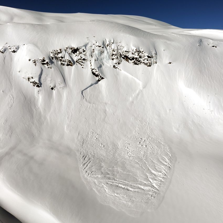
Abstract
    Avalanche forecasters need precise knowledge about avalanche activity in
large remote areas. Manual methods for gathering this data have scalability is-
sues. Synthetic aperture radar satellites may provide much needed complemen-
tary data. This report describes Avanor, a system presenting change detection
images of such satellite data in a web map client. Field validation suggests that
the data in Avanor show at least 75 percent of the largest avalanches in Scandi-
navia with some small avalanches visible as well.

                               Sammanfattning
    Lavinprognosmakare är i stort behov av detaljerad data gällande lavinaktivi-
tet i stora och avlägsna områden. Manuella metoder för observation är svåra att
skala upp, och rymdbaserad syntetisk aperturradar kan tillhandahålla ett välbe-
hövt komplement till existerande datainsamling. Den här rapporten beskriver
Avanor, en mjukvaruplattform som visualiserar förändringsbilder av sådan ra-
dardata i en webbkarta. Fältvalidering visar att datan som presenteras i Avanor
kan synliggöra minst 75 procent av de största lavinerna i Skandinavien och även
vissa mindre laviner.

                                       iii
Acknowledgements
Markus Eckerstorfer (NORCE Norwegian Research Centre) was external supervisor
and Josef Hallberg (Department of Computer Science, Electrical and Space Engineer-
ing at Luleå University of Technology) examiner for this degree project. Petter Palm-
gren (Swedish Environmental Protection Agency) and Jenny Råghall (Åre Avalanche
Center) provided valuable feedback regarding the project. Johan Jatko (Luleå Aca-
demic Computer Society) helped with computing resources and support while using
them. Nils von Sicard proofread the report.
Aron Widforss, Tromsø, May 2019
vContents
1 Introduction 1
1.1 Motivation . . . . . . . . . . . . . . . . . . . . . . . . . . . . . . . . . 1
1.2 Problem Definition . . . . . . . . . . . . . . . . . . . . . . . . . . . . 2
1.3 Delimitations . . . . . . . . . . . . . . . . . . . . . . . . . . . . . . . 4
2 Related Work 5
3 Theory 6
3.1 Avalanche Theory . . . . . . . . . . . . . . . . . . . . . . . . . . . . . 6
3.2 Avalanche Forecasting . . . . . . . . . . . . . . . . . . . . . . . . . . 6
3.3 Radar Theory for Avalanche Detection . . . . . . . . . . . . . . . . . . 10
3.4 Google Earth Engine . . . . . . . . . . . . . . . . . . . . . . . . . . . 16
4 Methods 19
4.1 System Overview . . . . . . . . . . . . . . . . . . . . . . . . . . . . . 20
4.2 Remote Analysis . . . . . . . . . . . . . . . . . . . . . . . . . . . . . . 21
4.3 Preprocessing . . . . . . . . . . . . . . . . . . . . . . . . . . . . . . . 25
4.4 Basemap . . . . . . . . . . . . . . . . . . . . . . . . . . . . . . . . . . 28
4.5 Web Client . . . . . . . . . . . . . . . . . . . . . . . . . . . . . . . . . 29
4.6 In Situ Validation . . . . . . . . . . . . . . . . . . . . . . . . . . . . . 30
5 Results 35
5.1 Validation Using the Swedish Avalanche Database . . . . . . . . . . . 35
5.2 Validation Using Tromsø Field Observations . . . . . . . . . . . . . . 37
6 Discussion 42
6.1 Validation . . . . . . . . . . . . . . . . . . . . . . . . . . . . . . . . . 42
6.2 Limitations . . . . . . . . . . . . . . . . . . . . . . . . . . . . . . . . 43
6.3 Operational Use . . . . . . . . . . . . . . . . . . . . . . . . . . . . . . 44
6.4 Dependencies . . . . . . . . . . . . . . . . . . . . . . . . . . . . . . . 45
7 Conclusions and Future Work 50
viiContents
8 References 51
A Pilot User Organisation I
A.1 Observersʼ Assessment of the System . . . . . . . . . . . . . . . . . . II
A.2 Infrastructure in Forecasting Areas . . . . . . . . . . . . . . . . . . . II
A.3 Daily Routine . . . . . . . . . . . . . . . . . . . . . . . . . . . . . . . III
B Client code overview IX
B.1 Back End . . . . . . . . . . . . . . . . . . . . . . . . . . . . . . . . . . IX
B.2 Front End . . . . . . . . . . . . . . . . . . . . . . . . . . . . . . . . . XIV
viii1
Introduction
In late 2017 the author was made aware of methods used by Swedish nordic skat-
ing enthusiasts to find ice to skate on. Skaters were using satellite-borne synthetic
aperture radar (SAR) data to determine whether specific areas were ice suitable for
skating, open water or snow covered areas (Österlund, 2017). The ice skating ap-
plication utilised radar backscatter as a tool for differentiating ground roughness
between distinct types of surfaces.
This project proposes that a similar methodology be used to detect avalanche de-
bris in mountain terrain. Avalanches are much more dramatic events than other
processes in the snowpack. As such they have the potential to create rapid and con-
siderable change in the snowʼs microwave scattering characteristics. This property
enables differentiation of avalanche debris from the surrounding area.
1.1 Motivation
Even in remote areas, mountain regions of Scandinavia are significantly populated.
Seasonal visitors add to the numbers. Recent improvements in ski equipment and
snowmobiles have attracted more people to higher and steeper terrain. According to
Hansson and Stephansen (2016) there are around 150,000 alpine tourers in Norway
alone. With the ever increasing numbers and improved access to remote areas the
risk to visitors has never been so high (Ormestad & Tarestad, 2018).
This situation has required authorities and organisations to strive to improve
measures to help visitors travel safely through mountainous regions. The Swedish
government has worked tirelessly with mountain safety ever since the catastrophic
accident in the Anaris mountains in 1978. The accident spurred the foundation of
the Mountain Safety Council of Sweden as well as the Swedish mountain rescue or-
ganisation. During their early life, mountain safety focused on relatively flat ter-
rain with higher visitor numbers. As equipment developed and habits changed the
authorities needed to keep pace. In the winter of 2016, following an updated gov-
ernment mandate, Swedish Environmental Protection Agency (SEPA) (2016) issued
its first set of avalanche forecasts covering three mountainous areas that were con-
sidered high risk. Prior to this, projects to establish forecasts had been undertaken
but scrapped due to lack of demand. The change in behaviour of skiers and the
11. Introduction
associated risks therein now made avalanche forecasting a fundamental and viable
proposition (Swedish Environmental Protection Agency (SEPA), 2016). An overview
of the SEPA operation can be found in Appendix A.
With limited resources and responsibility for vast areas, government agencies
needed effective tools for correct and reliable forecasts. Today, weather observations
and forecasts, snowpack observations and manual avalanche observations are used
extensively to produce regional avalanche forecasts. This forecast regime is essential
to skiers navigating mountain terrain as well as service personnel responsible for
operating critical infrastructure (e.g. roads and railway). Whilst a single forecast
may cover many square kilometers, current forecasters are limited to working with
only a few set of data points.
This lack of information may be remedied by providing more data points over
larger regions. Satellite based remote sensing would be an obvious tool for gathering
such detail and the European Space Agency (ESA) operates a number of satellites
which frequently cover large regions. The data gathered is of high-resolution and
readily available.
If data from forecasting areas were simplified and made available to forecasters
on a daily basis this would be hugely advantageous. Such data could be used to
provide more complete and reliable information on avalanche activity. In addition
to a tool for daily forecasting, it could be used to make statistical analysis of areas
and thereby providing insight into where and when avalanches may occur. It could
also be of use when studying the causal relationship between avalanche activity and
triggering factors. As data collection would be automated such an analysis could
potentially be done on a slope-by-slope basis.
1.2 Problem Definition
The project goal was to produce a solution for continually delivering current and
historical data on avalanche activity over large areas. In order to provide a working
model a series of distinct tasks were needed as outlined below:
• The satellite data delivered by ESA had to be calibrated, georeferenced and
orthorectified.
• An algorithm enabling the detection of avalanche debris had to be devised.
• Said algorithm needed to be implemented.
• A client presenting the generated data in a digestible manner had to be con-
structed.
The primary requirement of the system as a whole would be that trained users
were able to identify recent and historic avalanche debris.
Preprocessing Satellite data published by ESA are not referenced using geographic
coordinates. Therefore it would be necessary to fetch ESA data and calibrate, georef-
21. Introduction
erence and orthorectify it in a timely manner. To achieve this a server infrastructure
needed to continually check for published data and preprocess that data to an appro-
priate format that could then be used as input to the remote analysis algorithm. This
had to be done in near real-time as the value of the information degraded quickly.
Remote analysis algorithm The data contained information about backscatter (en-
ergy in the electromagnetic spectrum that the active radar sensor receives back from
the object it remotely senses). This was used as input to an algorithm, using backscat-
ter change over time to distinguish avalanche debris from smooth undisturbed snow.
Raster based arithmetic operations, such as subtraction of a reference image, could
be used to compare values over time and masks could delimit the areas to compute
to only cover avalanche terrain.
Remote analysis implementation The algorithm needed to be implemented in a
system that was scalable enough to cover vast areas and deliver the output to clients
in a prompt manner. An implementation using lazy evaluation would be highly
preferable since the algorithm would likely evolve over time. When an updated algo-
rithm was published, a lazy implementation would immediately serve the updated
output whereas an eager implementation would go through an enormous historic
dataset to serve the updated information.
As the solution could be used in other parts of the world the data and implemen-
tation was as generic as possible. This would, for example, mean that low-resolution
digital elevation models (DEM) would be preferred over high-resolution ones.
Client A good client should present the important data in a quick and readable way.
A low-latency presentation would likely need a caching strategy to be prepared in ad-
vance for requests. For the client to show readable information the radar data would
need to be supplemented with additional data. Such data would be topographic
basemaps and layers showing avalanche terrain.
The client would need to be usable on a variety of devices ranging from desktop
workstations to mobile devices. Whilst prospective users could have knowledge of
avalanche theory in order to assess features in the data that represent avalanche
debris, the data should not require users to know details regarding the origin and
collection of the data.
The area of interest for the project was the Scandinavian peninsula. The client
needed to present detailed data over this area in a prompt manner. The data pre-
sented needed to be both recent and historic to allow for detailed analysis.
31. Introduction
1.3 Delimitations
While this thesis depends heavily on underlying radar and avalanche theory, it is
not discussed in more detail than necessary. The subject of avalanche forecasting
is covered in Section 3.2 and Appendix A. The system developed makes no attempt
at assessing avalanche risk as this is the task of the system user and not the system
itself.
While the client will hopefully be sufficiently user-friendly to be used in oper-
ations, project success will not depend on usability but on objective measures of
avalanche debris detection. Even the best client is unable to present faulty data in
a good manner. The focus of the project will therefore be to measure how much of
the data generated is interpretable and not on the interface it is presented in.
An important part of assessing if data, or a model for interpreting data, is good is
to look at the frequency of false positives and false negatives. The plan for validat-
ing the data generated by Avanor is to compare it with observations from an external
avalanche observation database. While this makes it easy to find false negatives (the
database lists an avalanche that is not visible in the satellite data), false positives
need a more structured approach where data is interpreted first and then compared
with observations of non-occurring avalanches. Data regarding avalanches not be-
ing triggered is hard to find at the moment. A cost effective way in the future could
be to encourage avalanche forecasters to register areas where no avalanches were
present.
Other systems with the same objective as the one discussed in this thesis per-
form automated detection of avalanche debris. This is not a current priority in the
development of Avanor.
42
Related Work
Research regarding remote detection of avalanche debris has been conducted using
a variety of instruments and sensors. Eckerstorfer et al. (2016) described avalanche
debris detection using optical, laser and radar sensors from ground based, airborne
or spaceborne platforms. There has also been some detection schemes developed
using seismic (Bessason et al., 2007) as well as infrasonic sensors (Thüring et al.,
2015).
The most intuitive approach for avalanche debris detection is probably using op-
tical imagery where orthophotos are either manually interpreted or automatically
classified by an algorithm. Automatic optical methods may even exceed human ca-
pabilities in good conditions when working at scale (Lato et al., 2012). The prob-
lem with the methodology used is the dependency on the sparse resource of good
weather and in the case of airborne orthophoto, the practice of taking photos only
in the summer (Eckerstorfer et al., 2016). This dependency on good weather can be
remedied by using satellite synthetic aperture radar (SAR), which is largely weather
independent (Eckerstorfer et al., 2016). Wiesmann et al. (2001) showed the first ex-
ample of SAR being used to detect avalanche activity. They used a temporal change
detection scheme to show where avalanche debris had appeared. Since then rapid
improvements in satellite SAR technology have enabled higher-resolution data be-
ing available at a lower cost (Eckerstorfer et al., 2016). Using commercially available
data, debris from small avalanches can now be detected in individual images with-
out change detection (Eckerstorfer & Malnes, 2015).
Using radar images from ESAʼs two Sentinel-1 satellites, manual detection of the
complete avalanche activity of large areas is feasible to record over prolonged peri-
ods. (Eckerstorfer et al., 2017). Methods for automatic detection have been devised
(Vickers et al., 2016), updated (Vickers et al., 2017), and improved (Kummervold et
al., 2018).
Existing solutions provide vector representations or image files showing where
avalanche debris has been detected. This project tries to deliver the data on a map
interface instead. While Avanor will not have any automatic detection in the near
future, it may provide improvements in data discovery by allowing for a pan-and-
zoom interface instead of web server listings.
53
Theory
Avalanche forecasting and accident prevention is an interdisciplinary field covering
snow science, meteorology, physics, statistics, engineering, psychology and more.
This chapter covers what avalanches are, how they occur, the process of fore-
casting them, the relevant radar theory for detecting them and a tool for processing
radar images.
3.1 Avalanche Theory
An avalanche is a mass of snow that rapidly moves downslope (Jamieson, 2009).
Schweizer and Jamieson (2001) showed that the median slope angle for reported
human-triggered avalanches is 38° in Switzerland and 39° in Canada, with a quar-
tile distance of 4° in the union of the two datasets.
Avalanches are classified according to their type of release and the degree of
snow wetness (CAA, 2016). Dry slab avalanches release as a bulk after failure in a
weak snow layer that leads to sudden crack development and catastrophic collapse
of an overlying slab (Schweizer et al., 2016). Loose snow avalanches release from
a point after weakening of the surface snow. Both slab avalanches and loose snow
avalanches can occur in wet snow. Additionally overhanging snowdrifts, referred to
as cornices, can trigger both types of avalanche when they collapse and fall.
A slab avalanche may be triggered by artificial loading with pressure being applied
temporarily and locally (e.g. by a skier). This makes them the most dangerous type of
avalanche. Slab avalanches can also be triggered from gradual uniform loading (e.g.
precipitation) or from other natural triggers (e.g. surface warming) (Scheizer et al.,
2003). These natural processes alter the snow structure by weakening certain snow
layers or creating overburden stress on existing weak snow layers.
3.2 Avalanche Forecasting
Avalanches present a danger to travellers in steep snow covered terrain as well as
for infrastructure. Forecasts can help all affected parties to mitigate risk. Users of
avalanche forecasts can have very different objectives depending on the situation
63. Theory
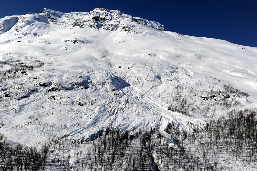
(a) Image of a wet slab avalanche that started just below the cliffs. It was triggered by a
collapsed cornice and continued downslope until the terrain was sufficiently flat to stop it at
the treeline.
(b) Image of a fracture line (the uppermost part of an avalanche) of
a dry slab avalanche visible below the cliffs. The image also shows
a stauchwall (marks the upper boundary of the debris) a small dis-
tance below the fracture line.
Figure 3.1: These avalanches were documented on April 5, 2019. The part of the avalanche detectable
by radar is the debris accumulation on the bottom of the avalanches. Photographs by Jakob Grahn,
NORCE.
73. Theory
and area. The reported forecast may include very different information depending
on the recipient.
3.2.1 Inputs
LaChapelle (1980) described avalanche forecasting as a multi-dimensional process
investigating a diverse set of factors integrated through time. The input data is often
redundant and correlated across input types. Three groups of data can be discerned:
meteorological data, snow-cover structural data and data about the mechanical state
of the snow. These groups are inherently interconnected since weather affects the
snowpack and thereby affects the movement of snow (LaChapelle, 1980).
The data samples must be collected as a time series, where data is extrapolated
into the future using external forecast services such as weather services, as well as
empirical knowledge and reasoning about processes in the snowpack. Data must be
collected over the whole area to assess the current conditions.
Most of the data collection is dependent on operators or observers, meaning that
the data density is biased to populated areas. This is where remote detection can be
of assistance, delivering data from remote areas as well as historical data, enabling
forecasters to prioritize resources in a more efficient manner.
Meteorological observations
A wide range of weather data is collected by forecasters. CAA (2016) defines obser-
vation guidelines for a range of parameters including:
• cloud cover,
• precipitation type, amount, intensity, mass and density,
• surface penetrability,
• air and snow temperatures,
• wind,
• blowing snow and
• barometric pressure.
Forecasters also make heavy use of general and specially made weather forecasts
and other organisationsʼ observations.
Meteorological data is widely available and easy to gather over large areas but
the relation between weather conditions and avalanche occurrence is not straight-
forward.
Snowpack observations
The snowpack is examined primarily by digging snow profiles and performing sta-
bility tests. Examples of such investigations are covered in Appendix A.3.2.
83. Theory
These tests provide a range of information regarding the state of degradation in
the snowpack as well as its susceptibility to collapse. The data is expensive to collect
and spatially variable (Schweizer et al., 2008). The extensive resources needed to
collect the data means that it is often extrapolated to large regions. On occasions
data from neighbouring forecasting areas may be used.
Avalanche observations
The recording of occurred avalanches is an important part of the data gathering pro-
cess. Avalanche activity is the most important indicator in assessing the current
snow stability. Avalanche activity is positively correlated with avalanche danger.
Thus frequency and type of avalanches can be used to determine snow stability on
a regional level.
Avalanche observations may be one of the more important aspects of the forecasts
for some users, specifically when planning fixed infrastructure. Such applications
require statistical data on large timescales and are not so dependent on the exact
situation at a specific time as other forecast recipients (CAA, 2016).
Both LaChapelle (1980) and CAA (2016) stress the importance of noting the non-
occurrence of avalanches. Data regarding non-occurring avalanches could be of
great importance when evaluating remote detection schemes.
3.2.2 Process
While the forecasting process varies depending on regional detail, Statham et al.
(2018) defined four sequential questions that all forecasters should tackle:
1. What type of avalanche problems exists?
2. Where are these problems located in the terrain?
3. How likely is it that an avalanche will occur?
4. How big will the avalanche be?
These questions should be sequentially applied on a range of temporal and spa-
tial scales. The question about likeliness can be phrased as, how likely are avalanche
occurrences in a specific valley over the course of a snow season? But the same question in
a different context can be more local, how likely is it that I will trigger an avalanche by
going down this gully? (Statham et al., 2018). The same scalability applies to the other
questions.
Sweden has followed a Canadian model when developing its forecasting service
(Ormestad & Tarestad, 2018). This model focuses on the hazards present in the ter-
rain, where a hazard is defined as a source of potential harm, or a situation with the po-
tential for causing harm (CAA, 2016), irrespective of the risk the hazard poses (Statham
et al., 2018). The meaning of risk in this context is defined as the probability and sever-
ity of an adverse effect (CAA, 2016). This means that the avalanche bulletin will not
93. Theory
take into account factors such as the population density or structures in avalanche
paths.
3.2.3 Outputs
Avalanche bulletins are often organized in a manner resembling an information pyra-
mid (WSL Institute for Snow and Avalanche Research SLF, 2018; Statham et al., 2018).
This means that the bulletin is fractal-like and starts with basic information that any-
one can comprehend (e.g. a five-level avalanche danger scale) and then proceed to
more detailed information to the point of almost presenting raw data. Such bul-
letins are conceptually created by taking the forecasterʼs assessment and repeatedly
streamlining the data until it reaches its simplest form.
When presenting the assessment the data must be customised to suit the receiver.
The users of the bulletins may mainly be skiers or might include those in charge
of infrastructure in the area. Such factors could affect the information included in
avalanche bulletins of different regions.
3.3 Radar Theory for Avalanche Detection
When detecting avalanches from satellite data, the debris is the part which is pos-
sible to detect. It is the depositional part of the avalanche. Detection of avalanche
debris in radar imagery is possible due to its high surface roughness, scattering more
energy back to the radar.
Synthetic aperture radar (SAR) uses a fast moving radar antenna to cover a region
with microwave signals. By using the Doppler effect experienced by the moving an-
tenna, the received signal can be processed to replicate one of a much larger station-
ary antenna (Woodhouse, 2006). The property recorded by the radar is backscatter
(the amount of the sent signal returned to the radar array from an object that is re-
motely sensed).
3.3.1 Microwave Scattering on Snow
Dry snow can be considered a low-density mesh of ice crystals. Woodhouse (2006)
tells us that the random structure of snow makes it act as spheres. The scattering
happens in all parts of the snow, both in layers and at layer boundaries. Water con-
tent will not affect the scattering characteristics of the snow due to the small relative
volume it occupies. It will however increase the dielectric constant of the medium
considerably increasing absorption and decreasing the share of the signal being scat-
tered and transmitted (Woodhouse, 2006).
Another factor affecting the scattering on snow is grain size (Woodhouse, 2006).
This is due to the changing ratio between the scattered signalʼs wave length and
the size of the scattering snow. All of the above apply to undisturbed snowpacks.
103. Theory
Eckerstorfer and Malnes (2015) inferred a model of backscatter from disturbed snow
(avalanche debris) both in wet and dry snow conditions (see Figure 3.2). In conclu-
sion, snow is a dynamic medium making it difficult to infer any one property from
the sensed backscatter (Woodhouse, 2006).
Backscatter as a proxy for surface roughness
One of the parameters that affects scattering in general is surface roughness. A
perfectly smooth surface will reflect most of the scattering in one specific direction
(the specular direction) just like a mirror (Woodhouse, 2006). The more rough a sur-
face, the more diffused the scattering becomes, scattering less in the specular di-
rection and more in other directions, such as the direction of the sensing satellite.
Woodhouse (2006) define a smooth surface according to the Rayleigh criterion as one
whose height has a standard deviation lower than a 1/4 of the wavelength used,
λ
hsmooth < (3.1)
8 cos θi
where hsmooth is the standard deviation of the surface, λ the wave length and θi the
incident angle. A more strict criterion often used is that of Fraunhoffer (Woodhouse,
2006), requiring a standard deviation lower than 1/8 of the wave length,
λ
hsmooth < . (3.2)
32 cos θi
This can be used, as the sensed backscatter will have a higher amplitude over
avalanche debris than over other areas. Provided the 5.405 GHz (ESA, n.d.-a) wave-
length used by Sentinel-1 and an inclination angle of 35°, this would mean that the
standard deviation of a smooth surface defined by the Rayleigh or Fraunhoffer cri-
terions would be no larger than 8.4 or 2.1 mm respectively. Variations in the snow
larger than this, which would be virtually any variation at all, would be measurable
as increased diffusion and sensed backscatter (see Figure 3.3).
3.3.2 Geometric Distortions
Avalanches tend to have the unfortunate property of only occurring in highly in-
clined terrain. This leads to a number of problems when trying to detect them with
radar since the local terrain scatters the signal in a non-optimal way. It is important
to understand that the perspective of a radar image is radically different from an op-
tical image due to the position of incoming data being determined by time and not
by refraction in a transparent medium.
Foreshortening
One of the distortions mentioned by Woodhouse (2006) occurs when the local in-
cidence angle is noticeably smaller than the general incidence angle. When this
113. Theory
(a) The backscatter of snow is a combination of ground and snow surface scattering as
well as scattering inside the snowpack.
(b) In dry, undisturbed snow, the bet- (c) In dry avalanche debris the signal
ter part of backscatter comes from signal still transmits through the snowpack, but
transmitted through the snowpack and the share of backscatter originating from
scattered by the ground surface. snow surface and volume scattering goes
up dramatically. This increase can be ex-
plained by the rough snow diffusing the
signal, leading to more scattering in the
direction of the receiver.
(d) Wet snow has a high dielectric (e) In wet avalanche debris, the rough
constant, severely limiting transmission surface diffuses the signal, increasing
through the medium and increasing backscatter. The medium is still impen-
absorption. This means that almost all etrable with high absorption.
of the backscatter originates from snow
surface scattering. As the surface is
smooth, most of the scattering goes in
the specular direction and backscatter
levels are low.
Figure 3.2: Diagram reproduced from Eckerstorfer and Malnes (2015).
123. Theory
(a) When the foil is smooth, almost all (b) A rough foil still reflects most of the
light is reflected away from the inclined light away from the camera, but enough is
camera and the foil appears dark. reflected back to make it appear brighter.
Figure 3.3: An aluminum foil is pictured with flash twice. The light reflected back to the camera de-
pends on the foilʼs roughness. As this happens on a sub-pixel scale when using radar, the individual
grooves are not visible in radar data, but still affect the pixelʼs overall value.
A′ B′ C′
Radar
A B C
Figure 3.4: The perspective of a radar. The front of the objects experience foreshortening, with layover
on A′. The backsides of B′ and C′ are hidden in radar shadow. Foreshortening will be most severe near
nadir, and radar shadow worst far from nadir (Woodhouse, 2006).
133. Theory
Figure 3.5: Sentinel-1 radar data showing layover (light areas) and radar shadow (dark areas). The data
is reprojected and orthorectified, so foreshortening compression and offset is mediated, with compres-
sion artefacts appearing on foreshortened areas instead.
occurs data is compressed and offset towards the nadir, the position of the satellite
projected onto the ground surface. This in turn leads to the backside of the object
taking up a disproportionately large area. The reason for this effect is the sonar-like
way SAR determines the position of the returned signal. The signal from the top of
the object will be returned in close temporal proximity to the signal from the lower
parts of the same object leading to the conclusion that the sensed parts are closer to
each other than they actually are. This effect can be of varying severity, see the dif-
ference between the projection of objects B and C in Figure 3.4. This effect is purely a
function of inclination and not the size of the object. Foreshortening is more preva-
lent close to the nadir due to the lower incidence angle (Woodhouse, 2006). This
issue can be addressed somewhat by orthorectifying the signal.
Layover
Layover is a special case where the top of an object is physically closer to the satel-
lite than the bottom. This results in data from the upper part of the object leaning
over the lower parts thereby appearing as if the top actually was strictly above the
bottom (see the projection of object A in Figure 3.4) (Woodhouse, 2006). Information
about the origin of the returned signal will be lost in such cases, a consequence of
projecting a three-dimensional environment onto a two-dimensional grid. As infor-
mation is missing the effect can not be corrected by orthorectification. The loss of
information is visible in Figure 3.5, where the bright areas contain artefacts and less
143. Theory
information.
Radar shadow
As SAR mostly uses a high general incidence angle the backside of objects will be
hidden behind their satellite-facing side. No signal will be returned from these ar-
eas and only noise will exist in imagery covering such regions, see the projection of
objects B and C in Figure 3.4 as well as Figure 3.5.
3.3.3 Sentinel-1
The Sentinel-1 mission by ESA images Earth using SAR (ESA, n.d.-a). It produces
imagery of resolutions down to 5 m/px and swath widths up to 400 km. The mis-
sion operates two satellites, Sentinel-1A and -1B. The first satellite was launched on
April 3, 2014 and the latter on April 26, 2016. They share the same orbital plane, but
are offset by half an orbital period. The satellites carry a right-looking C-band SAR
and orbit Earth in a near-polar sun-synchronous orbit. This means that the orbit
is of a high inclination, providing high-latitude areas with near-daily coverage. It
also implies that the orbit is fixed relative to the relationship between Earth and the
Sun. Specifically, the satellites always pass the time 18:00 on their southbound path,
providing imagery at dawn and dusk (ESA, n.d.-a).
The path the satellites take at dawn is south-southwest (descending path) and
the path at dusk is north-northwest (ascending path). These orbital properties de-
termine what slope aspects are affected by the geometric distortions described in
Section 3.3.2 and illustrated in Figure 3.4. As the radar is right-looking, descending
paths have eastern slopes closest to nadir, making them subject to foreshortening,
while western aspects are prone to radar shadow. The situation is reversed on as-
cending paths.
Sentinel-1 uses a radar that can send and receive using a vertically or horizon-
tally polarised signal (ESA, n.d.-c). Different materials have distinct polarisation sig-
natures and Sentinel-1 data preserves all combinations of polarisation in separate
layers. The naming scheme for these layers are a two letter combination of V and
H. For example the layer HV contains data that was transmitted horizontally and
received vertically. For Avanor, VH polarisation was arbitrarily chosen as the only
polarisation used.
This report uses the term period for the 12 days a satellite takes to cover all the
predefined tracks, effective period for the half-period it takes to cover the tracks by
both satellites and relative orbit for describing one of the 175 predefined tracks within
a period.
153. Theory
3.4 Google Earth Engine
Google Earth Engine (GEE) is a cloud-based platform for planetary-scale geospatial
analysis. It claims to bring Googleʼs massive computational capabilities to bear on
a variety of high-impact societal issues (Gorelick et al., 2017). It exposes massive
parallelism for remote analysis in a developer-friendly way by hosting most large
Earth observation datasets and exposing APIs for manipulating them.
The tool uses a special client-server model that can be confusing at first as it cre-
ates the illusion of work being done long before anything happens. In Listing 3.1 a
short example is presented of a program that runs equally well in the GEE sandbox
as by using its JavaScript (JS) API.
1 var sntl1 = ee.ImageCollection('COPERNICUS/S1_GRD_FLOAT')
2 // Select a small date range.
3 .filterDate(ee.Date('2018-12-24'), ee.Date('2018-12-27'))
4
5 // Use only the 'VH' band in the images.
6 .filter(ee.Filter.listContains('transmitterReceiverPolarisation', 'VH'))
7 .map(function(img) {
8 return img.select('VH');
9 })
10
11 // Merge all available images.
12 .mosaic()
13
14 // Scale to dB.
15 .log10()
16 .multiply(10);
17
18 // Fetch access tokens.
19 sntl1.getMap({ min: -25, max: 0 }, function(map, err) {
20 if (err) throw new Error(err);
21
22 console.log('MapId: ' + map.mapid);
23 console.log('Token: ' + map.token);
24 });
Listing 3.1: A basic GEE script.
In row 1 an ee.ImageCollection object is instantiated. This object contains no
images or even references to images. It is only an abstract representation for an
image collection available on GEEʼs servers.
Methods of this object are then used to build an abstract syntax tree of objects
around it. Elaborate programs can be assembled just by calling methods on such
objects.
As the API is written in an imperative language it is natural to believe that some
computation is done when a method is called. For example, it looks like a function
163. Theory
is mapped onto the object on row 7. Instead a JS object is returned representing
a server-side mapping of that function. A consequence of this is that doing client-
specific things such as calling console.log() within such a function will not work
correctly.
When the program is defined to our satisfaction we can register it with GEE. We
do that by calling the method getMap() in row 19. This is the first time GEE gets
to know anything about the program. The remote server parses the syntax tree and
either returns an object containing information of a newly published map service
or an error message. Even though we now have everything needed to look at the
output images, no output has yet been produced. GEE has merely parsed, validated
and cached our program in a way to enable swift, parallel execution.
The output is calculated on demand using the published map service. Using a
map viewer of our choice we can connect to the service and look at the imagery.
The tiles we request are computed when we request them, enabling us to define a
program using massive amounts of data. However as we only load so many tiles the
computational load on GEE remains low. Even if we zoom out the viewport to cover
the whole world, pyramiding will make sure that we barely use any data at all.
3.4.1 Control Flow
There are some control flow mechanisms available to us. The first argument passed
to the ee.Algorithms.If constructor decides which of the two additional argu-
ments the object evaluates to (row 16 in Listing 3.2).
1 var sntl1 = ee.ImageCollection('COPERNICUS/S1_GRD_FLOAT')
2 .filter(ee.Filter.listContains('transmitterReceiverPolarisation', 'VH'))
3
4 // We can select bands from collections. There is no need to map a function.
5 .select('VH');
6
7 // Calculate mean of all images in collection. It is incredibly expensive.
8 var heavyOp = sntl1.mean();
9
10 // This is the same operation as in Listing 3.1.
11 var normalOp = sntl1
12 .filterDate(ee.Date('2018-12-24'), ee.Date('2018-12-27'))
13 .mosaic();
14
15 // This is a control flow object analog to an if-statement.
16 var conditional = ee.Algorithms.If(
17 false, // Condition to evaluate.
18 heavyOp, // Run on true.
19 normalOp); // Run on false.
20
21 // Note the cast!
22 var db = ee.Image(conditional)
173. Theory
23 .log10()
24 .multiply(10);
25
26 db.getMap({ min: -25, max: 0 }, function(map, err) {
27 if (err) throw new Error(err);
28
29 console.log('MapId: ' + map.mapid);
30 console.log('Token: ' + map.token);
31 });
Listing 3.2: Demonstration of control flow and lazy evaluation in GEE.
As the condition is false the conditional object will evaluate to normalOp and
produce the exact same map as the code in Listing 3.1. heavyOp will never be evalu-
ated and the inclusion of such an expensive operation does therefore not affect the
performance of the returned map service. This is an example of the lazy evaluation
of GEE. As it happens with code written in an imperative language, where eager eval-
uation is almost foundational, it may be confusing to begin with and hard to debug.
As the conditional is an ee.Algorithms.If object and not an ee.Image it does
not have the methods defined for the latter. So even if the conditional will evaluate
to an ee.Image it has to be cast on row 22 for any ee.Image-specific method to be ap-
plied. This is not the case if the object is used as an argument of another method. So
ee.Image.constant(1).subtract(conditional) would have worked fine as the
receiving method casts the parameter automatically.
One more peculiarity of GEE is that a lot of code can be syntactically correct on
the client but generate an invalid processing graph on the server. One such exam-
ple would be to misspell the band name 'VH' in the argument list to the select()
method. The client side API can not know that the misspelled name is inaccurate
and so will pass it to the server which will then send the callback function an er-
ror on row 26 in Listing 3.2 even if the actual error happened on row 5. Since what
is sent to the server is a syntax tree and not literal code, information about where
the error happened is lost. The API can only tell what kind of error happened and
theoretically also some kind of stack trace, even if no such trace is implemented in
GEE.
184
Methods
In order to present the data in a timely manner a variety of software and hardware
was used to compute the various steps between the ESA delivery and final map pre-
sentation.
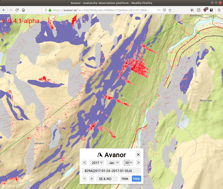
Figure 4.1: Avanor client UI, with radar signal difference (red), steep areas (purple), and a mask denot-
ing no signal due to layover or radar shadow (gray). The control panel on the bottom controls which
date data is presented for as well as which data to show if there are multiple overlapping data layers.
Basemap from Kartverket.
The result was a web client with a minimum of controls for adjusting image date,
layer selection where there was overlapping imagery and a help box (Figure 4.1).
This web client was located at https://avanor.se, and used an API at the same
web server to get information about where to fetch maps. These map sources could
be external, such as the basemap services, or served by GEE. In the case of GEE, the
194. Methods
web server had previously created and cached the location of a number of temporary
map services that it could send to the client. This process meant that the web server
never had to send any map data itself.
The user controls the client as a conventional web map by panning and zooming.
As soon as satellite data from a user-defined date intersects with the map viewport, it
is presented. The client also switches between data from different orbits seamlessly
as needed while navigating the map.
4.1 System Overview
The architectural challenge when delivering remote sensing analysis is one of scale.
Performing the analysis over a small area is relatively easy. However when expand-
ing the area of interest the system requirements quickly exceeds that of any single
albeit powerful machine. This can be addressed by building a parallel solution on
machines under ones own control or by outsourcing the problem of parallelism to a
third party. Avanor used a hybrid solution where one part of the work was performed
by a cluster of machines running at Luleå Academic Computer Society (LUDD) with
the storage, final calculations and styling of the maps outsourced to GEE using their
JS API.
Kartverket Lantmäteriet GEE Sentinel-1
Client https://avanor.se Ludd cluster ESA
Figure 4.2: The Avanor infrastructure. Dashed lines indicate metadata transfer and solid lines de-
note transfer of actual data. Google Earth Engine provided data layers. Lantmäteriet and Kartverket,
national mapping agencies of Sweden and Norway, provided basemaps for the client.
The work done locally on a cluster consisted of preprocessing the data published
by ESA, so that the location and value of each pixel in the images became known.
204. Methods
Once the preprocessing was complete, the images would be uploaded to GEE where-
upon a web server would continually instruct GEE to create routines for each im-
age, resulting in the coloured presentation seen in Figure 4.1. These routines were
then published as Web Map Tile Services (WMTS) by GEE on locations cached by
the web server. When a client later requested imagery of a given date and place, the
web server would check its cache for what WMTS service those parameters corre-
sponded to and return the location of that service together with the location of the
basemaps. The client would then assemble the different layers into a complete map
interpretable by the user. The different links between the computing resources are
illustrated in Figure 4.2.
4.2 Remote Analysis
The data available needed to be processed in a multitude of different ways. Whereas
masks delimiting avalanche terrain and geometric distortion were static and only
had to be computed once, the radar dataset needed constant updating and was com-
puted in near-real time.
4.2.1 Backscatter Difference Computation
Avalanche debris is possible to detect in individual radar images due to increased
backscatter reflected from them in comparison to surrounding, undisturbed snow.
By comparing two consecutive images sensed from an identical orbit, the change
induced by the avalanche debris can be isolated.
The whole algorithm was subject to GEEʼs lazy evaluation. This meant that the
algorithm was defined before it was run and then only evaluated for the areas the
client requested. To simplify the process Avanor did not care about single images. It
merged all images that were sensed in a single orbit since the division of data from
the same orbit into discrete images was arbitrary and of no value after ingestion
into GEE. This did not affect performance due to the lazy evaluation and general
architecture of GEE. The term image below therefore means such a merged stripe.
Avanor used a rather simple algorithm to generate its images. The first step was
to identify images to compare. Given an image i p,o in effective period p and relative
{ }
orbit o, a reference image could be found in R p,o = i p−n,o : n ∈ N, and n is small .
Avanor searched for an image i p−1,o or i p−2,o , images taken exactly one or two ef-
fective periods (6 or 12 days) before i p,o , preferring the shortest possible temporal
separation between the images. If an image r p,o ∈ R p,o was found, the image pair
was sent to the next step of the algorithm. The images used was of VH polarisation.
Only images from the same relative orbit o could be compared as the backscatter
characteristics are dependent on the geometry, i.e. the satellite had to sense from
the same location relative to ground for two images to be comparable.
214. Methods
A differential image d p,o = i p,o − r p,o was then calculated. As the value distribu-
tion was better suited for a logarithmic scale the resulting raster was logarithmised
into log10 d p,o . This also had the side-effect of discarding all negative change which
can be considered good for filtering as avalanche debris mostly exhibit a positive
backscatter change. The process of creating a differential image is illustrated in Fig-
ure 4.3.
When the raster had been logarithmised, a small number of adjustments were
made to make it better suited for presentation. The raster was scaled up, squared to
highlight larger differences and masked. All differences lower than −19.3 dB were
discarded from presentation. Differences larger than −2.9 dB were capped and pre-
sented as the strongest possible signal.
Finally, a mask was applied, delimiting avalanche runout zones where avalanches
are highly likely to occur. More specifically, the maskʼs valid areas were those within
350 m from a 20° slope and within 1 km from a 30° slope.
4.2.2 Layover and Shadow Mask Generation
As the application was focused on mountainous terrain a lot of the interesting ar-
eas were subject to layover and radar shadow (see Section 3.3.2). A mask had to be
constructed to remove unusable data from consideration. A number of different
techniques for generating such a mask were iterated over the course of the project.
This was necessary as more advanced services and hardware became accessible and
more knowledge regarding the subject was obtained.
Signal threshold layover mask When pointing a radar at a surface the backscat-
ter will decrease with an increasing angle of incident. This can be corrected using
terrain flattening which uses a terrain model to calculate the angle of incident and
scale the signal correspondingly (Braun, 2017). However such a correction can cause
problematic artefacts in mountainous terrain and is not used by GEE (2019c).
Layover mostly happens where the angle of incident is low. Therefore it was pos-
sible to create a mean from all available images in the GEE archive taken from the
same orbit and creating a layover mask using a threshold of the mean.
This mask was very coarse and removed too much information. Although it did
nothing to remove radar shadow it was better than not removing any data at all. A
part of it is presented in Figure 4.4a.
Local incident angle layover mask The GEE image archive contained bands for
angle of incidence relative to the ellipsoid. These could be combined with a ter-
rain model to generate a local angle of incidence (Greifeneder, 2018). Using such a
generated angle, a mask was created masking out everything that had an angle of
224. Methods
(a) Sentinel-1 image captured on January 24, 2017.
This was before an avalanche cycle and the image can
be used as a reference image.
(b) On January 30, 2017, multiple avalanches had oc-
curred and the debris was visible in light grey colours
due to relatively high backscatter.
(c) By subtracting the reference image Figure 4.3a
from the activity image Figure 4.3b a change detection
image can be produced. In this image, most of the sig-
nal appears to originate from avalanche debris.
Figure 4.3: Temporal change detection of avalanche debris in Sentinel-1 images of similar geometry,
with a 6-days repeat pass.
234. Methods
(a) This was the first layover mask used. It was com-
puted by taking a threshold of backscatter data. The
data was the average of all previous Sentinel-1 images
captured from relative orbit 66.
(b) This mask was generated by computing an esti-
mate of the local angle of incidence. Angles ≤ 20° was
masked.
(c) The last mask generated also included masking for
radar shadow (slightly darker gray). This was com-
puted by SNAP using Sentinel-1 metadata and terrain
models.
Figure 4.4: Masking of geometric distortions evolved over time. Gray denotes layover and radar masks
and purple covers unmasked areas with an inclination between 30–50°. The images show masks for
relative orbit 66. Basemap from Lantmäteriet.
244. Methods
incidence below 20°. This was much better than the previous mask but there was
still no masking for radar shadows, see Figure 4.4b.
SNAP layover and shadow mask When the cluster at LUDD became available in
April it was possible to use ESAʼs software suite SNAP to calculate a proper layover and
radar shadow mask using a terrain model. The terrain model used to create the mask
was the Norwegian DTM 10 Terrengmodell downsampled to a resolution of 50 m/px,
and two Swedish GSD-Höjddata, grid 50+ datasets, using the older photogrammetric
model where the newer laser scan lacked coverage. After the mask was generated it
was georeferenced and orthorectified using the ASTER and SRTM models to achieve
compatibility with GEE imagery. More information about the distinction between
the two latter terrain models is available in Section 4.3.2. For an example of this
mask, refer to Figure 4.4b.
In total over 700 recent radar images over Scandinavia were processed by SNAP
to create masks covering the whole peninsula. The masks were then combined per
relative orbit in GEE and saved as an asset available for GEE scripts.
4.2.3 Slope Layer
The Avanor client showed the user steep areas in a purple layer to assist in determin-
ing which backscatter signals occur in avalanche terrain (Figure 4.1). This layer was
generated by using the same Swedish and Norwegian merged terrain model men-
tioned in Section 4.2.2. A slope function was applied on the model and everything
between 30–50° was marked as steep. Anything steeper than 50° would most likely
be rocky and have very little snow, which is why the upper limit existed.
4.3 Preprocessing
The satellite data delivered by ESA was not georeferenced and had to go through a
thorough process before being usable.
The data used to create visualisations was of considerable size when supplying
imagery for multiple years. Due to this an already preprocessed archive maintained
by GEE was used for all visualisations older than a few days (GEE, n.d.). This archive
had a delay of a few days so it could not be used to supply daily images. Instead, up-
to-date images were produced on a server running SNAP, following the exact same
steps as GEE (2019c), to assure image compatibility since a reference image might
have been in the archive whilst the fresh image was not.
4.3.1 Downloading From ESA
Satellite images were available from ESA within hours of acquisition. A server con-
tinually polled the ESA archive looking for new images covering an area of interest.
254. Methods
This was done by a cron job running every 15 min. When a picture was published
by ESA, but missing in both the GEE long term archive as well as the short term col-
lection maintained by the author, it was logged to an on-disk datastructure so that
the next cron job would not try to process it again.1 As soon as a picture was found
it was downloaded to a server running the processing steps described below.
Download and polling was done using a Python library called sentinelsat. While
ESA provided a good API for querying the archive, the library provided batch down-
loading, checksum checking, retries on errors and conversion from GeoJSON to well-
known text (WKT) for search boundaries (Wille & Clauss, 2019, API Reference), which
made it worthwhile to add it as a dependency. It was so appealing that this part of
the project was written in Python to be able to use the sentinelsat library.
While all of the processing below was done with multiple images in parallel over
several computing nodes, the download was done sequentially due to download lim-
its imposed by ESA.
SNAP did have the capability to download restituted orbit files — describing the
satellite orbit in detail — and elevation models on demand. This functionality was
not very stable. Therefore, a complete elevation model over the processing area was
downloaded onto the servers beforehand and a short script queried ESA for the resti-
tuted orbit file, delaying the SNAP processing until the orbit file was published and
obtained.
4.3.2 Processing Images
The following steps were taken to preprocess imagery using SNAP so that it was
equivalent to archived GEE data.
Orbit file application An orbit file contains precise information about the actual
orbit the satellites were in when data was gathered. Several different orbital products
exists with varying precision and latency (Otten & Molina, 2018). The product used
for preparing images for Avanor were restituted orbit files, as they were provided in
near real-time.
The purpose of applying an orbit file was to adjust the projection of the data onto
an ellipsoid—a simplified earth model. This made sure that the boundaries of the im-
ages were correctly positioned. However, individual pixels would still be projected
to incorrect coordinates due to terrain features distorting the image.
1 This was implemented without any locks and introduced a potential race condition. The logging
was done within 30 s of job initialisation, and the jobs ran 15 min apart. However, there was a non-zero
risk of a race condition occurring involving one or more images sensed south of 60° N, as they would
be logged by a secondary script run after the northern images was all downloaded, something that
could happen at a multiple of 15 min. The worst possible scenario would lead to interference between
the two cron jobs, leading to a dropped image after retries due to incorrect checksums. Other possible
scenarios included images being processed twice. The second copy processed would then be dropped
on ingestion into GEE. The risk and consequences of such a situation were considered low.
264. Methods
GRD border noise removal When looking at Sentinel-1 data it is obvious that the
signal is incorrect near the borders of the swath. In this area, noise is abundant.
Therefore, the area within 500 meters of each edge was removed.
Thermal noise removal This operation was done to reduce discrepancies between
sub-swaths (GEE, 2019c). A sub-swath is a section of the sensing area, with a number
of sub-swaths running in parallel in the direction of travel to make up the 250 km
wide swath that is presented in the images downloaded from ESA (ESA, n.d.-c). The
radar cycled between these sub-swaths and scanned each from the back and forward
(ESA, n.d.-b).
Radiometric calibration The data in the images then had to be adjusted since a
variety of phenomena could affect the signal level at a specific point. The exact pa-
rameters were provided with the images in calibration look up tables. These specified
the parameters at given points and the areas between the points were interpolated
(ESA, n.d.-b).
Terrain correction When taking an optical aerial or satellite picture, the projec-
tion of the image is a central projection of one form of another. This means that
distances, angles and shapes are distorted in the image due to the position of the
camera. Furthermore, the terrain distorts the image, making a straight line appear
crooked. In such circumstances the images must be adjusted using a terrain model.
The operation of orthorectification takes the central projection and reproject it onto a
suitable geographical grid.
A radar image is not optical although a similar problem persists. As the situation
is purely geometrical, orthorectification has to be done in the case of radar as well.
This was a heavy operation done pixel by pixel whilst being aware of neighboring
terrain. Consequently, it is the main bottleneck of the program causing delay be-
tween the images being published on ESAʼs portal and new data being available on
Avanor.
The terrain model used by GEE (n.d.) was the Shuttle Radar Topography Mission
(SRTM) dataset, where it was available (between 56° S and 60° N), and ASTER Global
Digital Elevation Map outside of SRTM coverage. For the Avanor use-case, where im-
ages were processed for the Scandinavian peninsula, ASTER was the terrain model
used for the majority of orthorectification. This was true even if some avalanche
terrain in southern Norway had to be corrected using SRTM. These datasets were
used to assure an equal result to the images that would make itʼs way into the GEE
image archive some days later. If GEE equivalency had not been required the high-
resolution laser data and areal photogrammetric models issued by Scandinavian gov-
ernment agencies would have been used.
27You can also read