Brief communication: A double-Gaussian wake model
←
→
Page content transcription
If your browser does not render page correctly, please read the page content below
Wind Energ. Sci., 5, 237–244, 2020
https://doi.org/10.5194/wes-5-237-2020
© Author(s) 2020. This work is distributed under
the Creative Commons Attribution 4.0 License.

          Brief communication: A double-Gaussian wake model
                                 Johannes Schreiber, Amr Balbaa, and Carlo L. Bottasso
              Wind Energy Institute, Technische Universität München, 85748 Garching bei München, Germany
                                Correspondence: Carlo L. Bottasso (carlo.bottasso@tum.de)

                                   Received: 9 August 2019 – Discussion started: 23 August 2019
                        Revised: 3 December 2019 – Accepted: 8 January 2020 – Published: 14 February 2020

       Abstract. In this paper, an analytical wake model with a double-Gaussian velocity distribution is presented,
       improving on a similar formulation by Keane et al. (2016). The choice of a double-Gaussian shape function is
       motivated by the behavior of the near-wake region that is observed in numerical simulations and experimental
       measurements. The method is based on the conservation of momentum principle, while stream-tube theory is
       used to determine the wake expansion at the tube outlet. The model is calibrated and validated using large eddy
       simulations replicating scaled wind turbine experiments. Results show that the tuned double-Gaussian model is
       superior to a single-Gaussian formulation in the near-wake region.

1   Introduction                                                   ered the industry standard (Keane et al., 2016). The model
                                                                   was first introduced by Jensen (1983) and later further de-
                                                                   veloped by Katić et al. (1986). Other widely used and cited
Analytical engineering wind farm models are low-fidelity           wake models include the Frandsen model (Frandsen et al.,
approximations used to simulate the performance of wind            2006), the FLORIS model (Gebraad et al., 2014), and the
power systems. A wind farm model includes both a model             EPFL Gaussian models (Bastankhah and Porté-Agel, 2014,
of the wind turbines and a model of the modifications to           2016).
the ambient flow induced by their wakes, together with their          All such models have been designed to faithfully repre-
mutual interactions. Analytical wake models, as opposed to         sent the average flow properties of the far-wake region. How-
high-fidelity computational fluid dynamics (CFD) models,           ever, in the near wake (which is usually defined as the region
are simple, easy to implement, and computationally inexpen-        up to about 4 diameters (4 D) downstream of the rotor disk),
sive. In fact, they only simulate macroscopic average effects      the models seem to lack accuracy. Nowadays, onshore wind
of wakes and not their small scales or turbulent fluctuations.     farms tend to be closely packed, and turbine spacing often
Engineering wake models find applicability in all those cases      reaches values close to or even below 3 D (Schreiber et al.,
that do not need to resolve small spatial and fast temporal        2018; energiespektrum.de, 2015). This raises the necessity
scales, such as the calculation of the power production of a       of developing models that accurately represent the wake not
wind plant over a sufficiently long time horizon. Such models      only far away from the rotor disk but also in the near and
are also extremely useful in optimization problems, where a        mid-wake regions.
large number of simulations might be required before a so-            Keane et al. (2016) developed a wake model featuring a
lution is reached or where calculations need to be performed       double-Gaussian velocity deficit distribution in an attempt
on the fly in real time. Analytical wake models are thus of-       to formulate a model that closely resembles observed speed
ten utilized in wind farm layout planning and in the emerg-        distributions in both the near- and far-wake regions. In fact,
ing field of wind farm and wake control (Scholbrock, 2011;         while a single-Gaussian function is considered to be a good
Churchfield, 2013; Boersma et al., 2017).                          approximation of the wake velocity distribution in the far
   Because of their indisputable usefulness, engineering           wake (Bastankhah and Porté-Agel, 2014, 2016), the near
wake models have been extensively studied in the literature.       wake is better approximated using a double-Gaussian dis-
The Jensen (PARK) formulation is one of the most widely            tribution. This is due to the presence of two minima in the
used wake models, to the extent that it is sometimes consid-

Published by Copernicus Publications on behalf of the European Academy of Wind Energy e.V.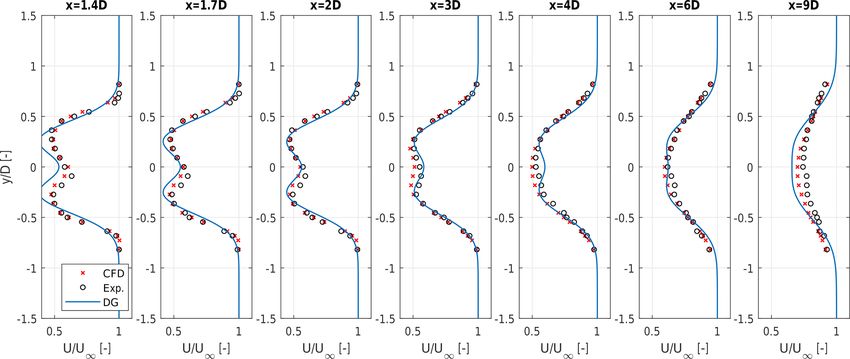
238                                                 J. Schreiber et al.: Brief communication: A double-Gaussian wake model

speed profiles close to the rotor disk, as also observed in ex-
perimental measurements and high-fidelity CFD simulations
(Wang et al., 2017). The double-Gaussian model by Keane
et al. (2016), which is referred to as the Keane model in this
paper, was developed in a similar fashion to the EPFL Gaus-
sian model (Bastankhah and Porté-Agel, 2014), and it was
intended to respect the principles of mass and momentum
conservation.
   In this short note, a double-Gaussian wake model, based
on Keane’s model and with emphasis on near-wake flow be-
havior, is derived, calibrated, and validated. The present for-
mulation addresses and resolves some issues found in the          Figure 1. Stream tube with nomenclature: U∞ is the ambient wind
original implementation of Keane et al. (2016), primarily         speed; U (x, r) is the local flow velocity in the wake at the down-
concerning momentum conservation. In addition, the wake           stream position x and radial distance r from the wake centerline;
expansion function is defined such that mass flow deficit con-    ṁ is the mass flow rate through the stream tube; AW is a planar
servation is achieved at the stream-tube outlet.                  cross-sectional area large enough to contain the wake deficit; A0 is
   This paper is organized as follows. The derivation of the      the rotor disk area; and T is the thrust force (by the principle of ac-
double-Gaussian wake model is detailed in Sect. 2, along          tion and reaction, an equal and opposite force is applied by the rotor
with the formulation of the wake expansion function. In           onto the flow).
Sect. 3, the model is tuned and validated, using both ex-
perimental measurements obtained with scaled models in a
                                                                  center, is defined as
boundary layer wind tunnel and by numerical results of high-
fidelity large eddy simulations (LESs). Additionally, the per-                    1  D+             −(r ± r0 )2
formance of the double-Gaussian model is compared to a            g(r, σ (x)) =      e + e D− , D ± =             ,                  (2)
                                                                                  2                    2σ 2 (x)
standard single-Gaussian formulation. Concluding remarks
and future work recommendations are given in Sect. 4. Fi-         where r0 is the radial position of the Gaussian extrema. The
nally, Appendix A derives some integrals appearing in the         standard deviation of the Gaussian function, noted σ (x), rep-
formulation.                                                      resents the width (cross section) of each of the two single-
                                                                  Gaussian profiles. The wake expands with downstream dis-
                                                                  tance x, causing the transformation of the initial double-
2     Wake model description                                      Gaussian profile in the near wake, through a flat-peak tran-
                                                                  sition region, into a nearly single-Gaussian profile in the far
2.1    Double-Gaussian velocity deficit                           wake. The wake expansion function is discussed in further
                                                                  detail in Sect. 2.2. A possible improvement to the present
The double-Gaussian wake model is derived in a similar way        model might include an azimuth-dependent double-Gaussian
to the Frandsen (Frandsen et al., 2006) and EPFL single-          function. This would allow one to model a non-axisymmetric
Gaussian models (Bastankhah and Porté-Agel, 2014). Fol-           double-peaked wake profile, caused by a sheared inflow
lowing their approach, the conservation of momentum prin-         and/or by the misalignment of the rotor axis with respect to
ciple is applied on an ansatz velocity deficit distribution,      the wind, at the cost of extra tuning parameters.
which includes an amplitude function. Thereby, an expres-            The conservation of momentum principle is now applied
sion for the amplitude is obtained that assures conservation      on the ansatz velocity deficit distribution, using the ampli-
of momentum.                                                      tude function C(σ (x)) as a degree of freedom. Accordingly,
   At the downstream distance x from the wind turbine ro-         the axial thrust force T is related to the rate of change of mo-
tor and at the radial distance r from the wake centerline, the    mentum p of the flow throughout the stream tube (see Fig. 1),
wake velocity deficit U∞ − U (x, r) is modeled as the prod-       i.e.,
uct of the normalized double-Gaussian function g(r, σ (x)),                               Z
                                                                        dp
which dictates the spatial shape of the deficit, with the am-     T =       = ṁ1Ũ = ρ U (x, r) (U∞ − U (x, r)) dAW , (3)
plitude function C(σ (x)). This yields                                  dt
                                                                                           AW

U∞ − U (x, r)                                                     where ṁ is the mass flow rate through the stream tube, 1Ũ
              = C(σ (x))g(r, σ (x)),                       (1)
   U∞                                                             an effective wake velocity deficit, ρ the air density, and AW a
                                                                  planar cross section at least large enough to contain the wake
where U∞ represents the ambient wind speed and U (x, r) the       deficit. Equation (3) is only valid if there is an equal pres-
local flow velocity in the wake. The double-Gaussian wake         sure and negligible flow acceleration at the inlet and outlet
shape function, which is symmetric with respect to the wake       sections of the stream tube and, additionally, if shear forces

Wind Energ. Sci., 5, 237–244, 2020                                                          www.wind-energ-sci.net/5/237/2020/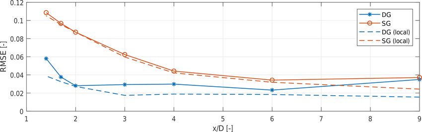
J. Schreiber et al.: Brief communication: A double-Gaussian wake model                                                       239

on the control volume can be neglected. The thrust force T         2.2   Wake expansion function
is customarily expressed through the nondimensional thrust
coefficient CT as                                                  In the previous section, following the conservation of mo-
                                                                   mentum, the shape of the double-Gaussian wake deficit has
   1     2                                                         been defined as a function of the Gaussian parameter σ . In
T = ρA0 U∞ CT ,                                             (4)
   2                                                               this section, a wake expansion function σ (x) is introduced,
                                                                   which is linear with respect to the downstream distance x.
where A0 is the rotor swept area.                                  By mass conservation, the wake expansion at the position of
   If the wake velocity, defined in Eqs. (1) and (2), is substi-   the stream tube outlet is therefore identified.
tuted into the Eq. (3), one obtains                                   In previous work by Frandsen et al. (2006) and Bastankhah
                                                                   and Porté-Agel (2014), stream tube theory was employed
                  Z∞
         2                       C(σ )                             to derive an equation for the initial wake width at the tur-
T  = ρπ U∞ C(σ )     eD+ + eD− −                                   bine rotor. Thereby, the number of tunable parameters of the
                                  2
                  0                                                wake expansion function is reduced, facilitating model cali-
                                                                   bration. However, this approach includes the assumption that

   e2 D+ + e2 D− + 2eD+ +D− r dr.                           (5)
                                                                   the stream tube outlet is located exactly at the turbine rotor
                                                                   itself, which is hardly true. Results indicate that the derived
Note that as the double-Gaussian wake expands all the way          initial wake width is too large to fit experimental measure-
to infinity, the integral boundary is set accordingly. The inte-   ments, which in turn requires a model retuning (Bastankhah
gration of Eq. (5), whose details are provided in Appendix A,      and Porté-Agel, 2014).
yields                                                                In the present work, the stream tube outlet is not assumed
        2                                                          to be located at the turbine rotor (x = 0) but at the unknown
T = ρπ U∞ C(σ ) (M − C(σ )N ) ,                             (6)
                                                                   downstream position x0 . Therefore, the expansion function is
                                                                   defined as
where

            2
                 −r02    √

                                           r0
                                                                  σ (x) = k ∗ (x − x0 ) + ,                                 (9)
M = 2σ e         2σ 2   + 2π r0 σ erf √          ,         (7a)
                                            2σ
                −r02
                         √                                         where parameter k ∗ controls the rate of expansion, while
        2                  π          r
                                        0
N =σ e          σ2     +     r0 σ erf      .               (7b)    represents the wake expansion at x0 . The wake expansion
                          2            σ                           function is assumed to be linear as in Bastankhah and Porté-
By substituting the thrust given by Eq. (4) into Eq. (6), and      Agel (2014).
solving the resulting quadratic equation for the amplitude            To derive , mass conservation between the Betz stream
function C(σ ), one obtains                                        tube and the wake model is enforced. Starting from Eq. (3),
                                                                   Frandsen et al. (2006) and Bastankhah and Porté-Agel (2014)
                                                                   show that the mass flow deficit rate at the outlet of a Betz
                          q
                       M ± M 2 − 12 N CT d02
C± (σ (x)) =                                   ,            (8)    stream tube (noted ST) can be written as
                                2N
             √
                                                                              Z
                                                                                    U∞ − UST
where d0 = 4 A0 /π is the rotor diameter. Both solutions           ṁST = ρ                  dAST
of the amplitude function C(σ ) would theoretically lead to                           U∞
                                                                              AST
the conservation of momentum at all downstream distances.                            s      !
However, the velocity profiles obtained by using C+ (σ ) are                π 2          2
                                                                         = ρ d0 β 1 − 1 − CT ,                               (10)
characterized by a negative speed (i.e., in the direction op-               8            β
posite to the ambient flow), and thus C+ (σ ) is deemed to
be a nonphysical solution. Therefore, the true solution for
                                                                   where UST is the uniform cross-sectional wake velocity. In
the amplitude function is C− (σ ). In addition, a momentum-
                                                                   this expression, β is the ratio between the stream tube outlet
conserving solution exists only if M 2 − 1/2 N CT d02 ≥ 0,
                                                                   area AST and the rotor disk area A0 , which can be expressed
which might not always be the case for large values of CT .
                                                                   as a function of the thrust coefficient CT as
   The derived expressions for M and N presented in this
paper differ from the results reported in the original publica-                  √
tion by Keane et al. (2016), even though all assumptions are          AST   1 1 + 1 − CT
                                                                   β=     =     √        .                                   (11)
identical. The expressions reported in the original paper were        A0    2     1 − CT
also evaluated numerically, yielding nonphysical results that
violate the conservation of mass and momentum underlying             At the Betz stream tube outlet (x = x0 ), the mass flow
the formulation.                                                   deficit rate of the double-Gaussian (noted DG) wake model

www.wind-energ-sci.net/5/237/2020/                                                          Wind Energ. Sci., 5, 237–244, 2020
240 J. Schreiber et al.: Brief communication: A double-Gaussian wake model
3 Model calibration and validation
3.1 Experimental and simulation setup
To calibrate and validate the double-Gaussian wake model,
time-averaged flow measurements from an LES numerical
solution have been used. The CFD simulation replicates
an experiment conducted with the scaled G1 wind turbine
(Campagnolo et al., 2017, 2019), which has a 1.1 m rotor di-
ameter and a 0.8 m hub height. Its design operating tip speed
ratio is 8 and its rated rotor speed is 850 rpm. The G1 model
is designed such that the characteristics of its wake are real-
istic in terms of shape, velocity deficit, and recovery. In ad-
dition, the model features closed-loop pitch, torque and yaw
control, and load sensors located at the shaft and tower base
(Campagnolo et al., 2017). The experiment was conducted
with a single G1 wind turbine model in the 36 m × 16.7 m ×
Figure 2. Visualization of the width of the double-Gaussian func- 3.84 m boundary layer wind tunnel at Politecnico di Milano.
tion at the stream tube outlet, as a function of the thrust coefficient The wake profile was measured using hot-wire probes at
CT and the position of the Gaussian extrema r0 . the downstream distances x/D = {1.4, 1.7, 2, 3, 4, 6, 9}
from the turbine. At each downstream location, the velocity
was measured at hub height at different lateral positions y
and then time averaged to obtain a steady-state value. The
ambient wind velocity within the wind tunnel was measured
writes as
using a pitot tube placed upwind of the G1 model. The wind
tunnel experiment was conducted with a 5 m s−1 hub height
Z wind speed, a power law exponent of 0.144, and a turbulence
U∞ − U (x0 , r) intensity of approximately 5 %, with the wind turbine oper-
ṁDG = ρ dAW
U∞ ating at CT ≈ 0.75.
AW
q A complete digital copy of the experiment was developed
M() − M()2 − 12 N()CT d02 with the LES simulation framework developed by Wang et al.
= ρπ M() . (12) (2017), which includes the passive generation of a sheared
2N() and turbulent flow, an actuator line model of the wind tur-
bine implemented with the FAST aeroservoelastic simula-
tor (Jonkman and Buhl Jr., 2005) and the tunnel walls. The
By equating both mass flow deficits (i.e., ṁDG = ṁST ), the simulation model includes also a slight lateral nonunifor-
initial wake expansion can be derived. The solution was mity of the inflow, in the form of a 2.7 % horizontal shear,
computed numerically as a function of the thrust coefficient caused by the wind tunnel internal layout upstream of the
CT and the spanwise location of the Gaussian extrema r0 . test chamber and by the tunnel fans. The proposed double-
The resulting surface is presented in Fig. 2. Note that the Gaussian wake model was calibrated and validated using
solution to stream tube theory is defined only in the range time-averaged CFD simulation results at the same down-
0 ≤ CT < 1, and tends to infinity as the thrust coefficient stream distances as the experiments, numerical and experi-
approaches the value of 1, due to mass conservation. mental measurements being in excellent agreement with each
The remaining parameters, x0 and k ∗ , in the linear wake other.
expansion function expressed by Eq. (9) are not explicitly
modeled, and they should be tuned based on experimental
measurements or high-fidelity simulations, as shown in the 3.2 Parameter identification and results
next section. Note that the underlying momentum conserva-
tion statement expressed by Eq. (3) has only been defined The double-Gaussian model proposed in this work has three
for ambient pressure. Therefore, the formulation is, strictly tunable parameters: k ∗ , x0 , and kr . Parameters k ∗ and x0 are
speaking, only valid for x ≥ x0 . However, as pressure recov- used to describe the wake expansion downstream of the tur-
ers rapidly immediately downstream of the rotor, reasonable bine rotor, as expressed by Eq. (9). The third parameter, kr ,
approximations can also be expected for x < x0 . Finally, k ∗ is defined as r0 = kr /2, and it describes the position of the
is expected to depend on atmospheric conditions (Peña et al., Gaussian extrema. When kr = 1 the curve extrema are lo-
2016) and turbine thrust (Campagnolo et al., 2019). cated at the tip of the rotor blades, while for kr = 0 the two
Wind Energ. Sci., 5, 237–244, 2020 www.wind-energ-sci.net/5/237/2020/J. Schreiber et al.: Brief communication: A double-Gaussian wake model 241
Table 1. Identified model parameters. the identified parameters, which in turn produce wake pro-
files that are fairly similar to the ones presented here. On the
Operating conditions Parameters other hand, identifying the model using only data points from
the far wake resulted in better fitting results at 9 D but with
U∞ (m s−1 ) CT (–) k ∗ (–) x0 (D) kr (–)
either very small values of r0 – which led to nearly single-
5.00 0.75 0.011 4.55 0.535 Gaussian profiles – or with high values of the k ∗ expansion
slope – which led to nonphysical solutions of Eq. (8) for the
amplitude function in the near-wake region, due to exces-
sively small Gaussian widths.
Gaussian functions coincide at the wake center, leading to a Figure 4 depicts with a solid blue line and ∗ symbols the
single-Gaussian wake profile. root mean square error (RMSE) between the DG wake model
In the original formulation by Keane, kr was fixed at 75 % (based on the parameters reported above, obtained from mea-
blade span, as it was argued that most lift is extracted from surements at 1.7, 3, and 6 D) and the reference CFD data as
the flow at this location. In the present work the parameter is a function of downstream distance. To identify a lower error
tuned based on measurements, as the assumed 75 % blade- bound, the DG wake model parameters were also tuned sep-
span position did not lead to satisfactory results. arately at each downstream distance, obtaining seven differ-
The goal of model calibration is to ensure that the wind ent local parameterizations. The corresponding RMSE with
velocity profiles match the reference data set as closely as respect to the CFD solution is reported in the same figure us-
possible. To this end, the squared error between the wake ing a dashed blue line. The small difference between the two
model and CFD-computed wake profiles is minimized with curves shows that the single (global) parameterization com-
respect to the free parameters. This estimation problem was puted using only three distances is only marginally subopti-
solved using the Nelder–Mead simplex algorithm imple- mal, in the sense that it is very close to the best possible fit-
mented in the MATLAB function fminsearch (Lagarias ting that a double-Gaussian shape function can achieve. The
et al., 1998). To ensure the generality of the results, only a plot shows also a slight increase in the difference between
subset of the reference data was used for parameter estima- the two curves in the far-wake region, which can again be
tion (namely the downstream distances 1.7, 3, and 6 D), while attributed to the fact that only one large-distance (6 D) mea-
the others were used for verification purposes. surement was used in the global tuning.
The identified parameters are presented in Table 1. The As a comparison, Fig. 4 also shows the results obtained
Gaussian extrema were found to be at approximately 53.5 % with the EPFL single-Gaussian (SG) model (Bastankhah and
of blade span (kr = 0.535), while the wake width at x0 is = Porté-Agel, 2014). The SG model was identified with the
0.23 D. Model calibration also resulted in the positioning of same procedure and measurements used for the DG model,
the stream tube outlet at x0 = 4.55 D, which appears to be a obtaining SG = 0.3177 and kSG ∗ = 0.0082; the correspond-
realistic value for the investigated turbine. ing RMSE with respect to the CFD results is reported in
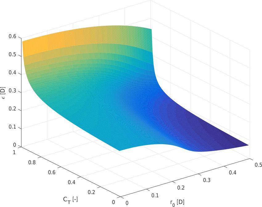
Figure 3 shows the experimental wake measurements us- the figure using a solid red line with circles. The lower er-
ing black circles, for all available downstream distances. The ror bound for the SG model, here again obtained by tun-
CFD results, shown using red × symbols, are almost identi- ing the parameters independently at each one of the seven
cal to the experimental measurements, highlighting the qual- available downstream distances, is shown using a dashed red
ity of the LES simulations. The predictions of the double- line. As expected, the SG wake model shows a significantly
Gaussian model are shown in solid blue lines. larger RMSE in the near-wake region than in the DG case.
The model exhibits good generality, as demonstrated by In fact, here the wake profile is indeed characterized by two
the good matching of the profiles at distances that were not peaks, so that the double-Gaussian shape function allows for
used for model estimation. Especially in the near-wake re- a more precise representation of the actual flow characteris-
gion up to about 3 D, the placement of the Gaussian extrema tics. Here again it should be noted that the difference between
appears to be in good agreement with the measured one. the global and local parameterizations is quite small, which
The performance of the model clearly depends on the data strengthens the conclusion that improved results are due to
used for its calibration. Using reference data close to the tur- the ansatz velocity deficit distribution and not to the specific
bine rotor is important for accurately gauging the positions of parameterizations. Comparing the SG with the DG model,
the velocity profile extrema, while a wider rage of distances Fig. 4 shows that both reach very similar RMSEs for 9 D.
leads to an improved expansion behavior. In the present case, The similarity between the two models continues for larger
more data from the near-wake region (1.7 and 3 D) were con- downstream distances.
sidered in the tuning process than in the far wake (6 D). This
leads to a slight overestimation of the velocity deficit at 9 D,
which could be attributed to an underestimation of the ex-
pansion slope k ∗ . However, tuning the model using the entire
set of reference data points leads to only small differences in
www.wind-energ-sci.net/5/237/2020/ Wind Energ. Sci., 5, 237–244, 2020242 J. Schreiber et al.: Brief communication: A double-Gaussian wake model
Figure 3. Normalized wind velocity profiles of the double-Gaussian model (solid blue line) compared to experimental measurements (black
circles) and CFD simulations (red × symbols). The distances 1.7, 3, and 6 D were used for model calibration.
Figure 4. Root mean square error between the reference CFD velocity deficit data and the engineering wake models. Double-Gaussian (DG)
wake model identified using measurements at 1.7, 3, and 6 D: solid blue line with ∗ symbols. DG wake model parameterized locally at each
downstream distance: dashed blue line. Single-Gaussian (SG) EPFL wake model identified using measurements at 1.7, 3, and 6 D: solid red
line with circles. SG EPFL wake model parameterized locally at each downstream distance: dashed red line.
4 Conclusions the far wake, a slight overestimation of the wake deficit could
be observed. It is speculated that this might be due to the
wake expansion gradient being slightly different in the near-
This short paper presented an analytical double-Gaussian
and far-wake regions. This claim, however, would need ad-
wake model. The proposed formulation corrects and im-
ditional work to be substantiated. The different shape of the
proves a previously published model proposed by Keane
wake in the near- and far-wake regions also suggests stitching
et al. (2016). The shape of the velocity deficit distribution
the two models together, the double Gaussian being used in
in the wake is described by two Gaussian functions, which
the near-wake region and the single Gaussian further down-
are symmetric with respect to the wake center, while the am-
stream. This would avoid the need for a single tuning that has
plitude of the velocity deficit is derived using the principle of
to cover such a long distance and different behaviors. Addi-
momentum conservation. A linear expansion of the width of
tional future work could extend the wake model to include
the Gaussian profiles was assumed, and stream tube theory
wake deflection, which could be done in a rather straight-
was used to estimate the conditions at the stream tube outlet.
forward manner by following Bastankhah and Porté-Agel
The model was calibrated and validated using a set of
(2016). In this case, a nonsymmetric double-Gaussian shape
time-averaged CFD simulation results, which replicate wind
function could be used to model the kidney shape of a de-
tunnel experiments performed with a scaled wind turbine in
flected wake (Bartl et al., 2018). More in general, an azimuth-
a boundary layer wind tunnel. Results show that the model
dependent double Gaussian might be used to account for the
fits the reference data with good accuracy, especially in the
effects of both misalignment and a sheared inflow.
near-wake region where a single-Gaussian wake is unable to
describe the typically observed bimodal velocity profiles. In
Wind Energ. Sci., 5, 237–244, 2020 www.wind-energ-sci.net/5/237/2020/J. Schreiber et al.: Brief communication: A double-Gaussian wake model 243
Appendix A: Integration of the momentum flux and its integral is computed as
conservation formula √ R
π r0 σ erf r−r
−(r−r0 )2 √ 0
2σ
Equation (5) can be written as I2 = lim −σ 2 e + 2σ 2 √ , (A8a)
R→∞ 2
0
2
T = ρπ U∞ C(σ ) (M − C(σ )N ) , (A1) −r02
√
2π r 0 σ −r 0
= σ 2 e 2σ 2 + erfc √ . (A8b)
2 2σ
where
Combining the previous results, one gets Eq. (7a), i.e.,
Z∞
−r02
√
M= eD+ + eD− rdr, (A2a) r0
M = I1 + I2 = 2σ 2 e 2σ 2 + 2π r0 σ erf √ . (A9)
0 2σ
Z∞
1 2 D+ A2 Derivation of N
N= e + e2 D− + 2eD+ +D− rdr. (A2b)
2
0 Term N can be split into three terms
1
In the following, integrals M and N are solved to obtain N= (I3 + I4 + 2I5 ) . (A10)
Eq. (7a) and (7b). 2
Terms I3 and I4 are collectively defined as
Z∞
A1 Derivation of M
I3 + I4 = e2 D+ + e2 D− rdr
M can be split into two terms: 0
ZR −(r+r0 )2 −(r−r0 )2
M = I1 + I2 . (A3)
= lim re σ2 + re σ2 dr. (A11)
R→∞
Term I1 is defined as 0
Solving the integral yields
Z∞ ZR −(r+r )2 !
0 h −σ 2 −(r+r0 )2 −(r−r0 )2
D+
I1 = e rdr = lim re 2σ 2 dr. (A4) I3 + I4 = lim e σ2 +e σ2
R→∞
0 0
R→∞ 2
√ i
π r + r0 r − r0 R
−(r±r0 )2 − r0 σ erf − erf , (A12a)
Noting that D± = 2σ 2 (x)
, one gets 2 σ σ 0
−r02
√ r
0
√ R = σ 2e σ2 + π r0 σ erf . (A12b)
σ
r+r
π r0 σ erf
−(r+r0 )2 √ 0
2σ
I1 = lim −σ 2 e 2σ 2
− √ , (A5a) Finally, I5 is defined as
R→∞ 2
0
Z∞ ZR
−r02
√ −(r+r0 )2 (r−r0 )2
−
2 2σ 2 2π r0 σ r0 I5 = e D+ +D−
rdr = lim re 2σ 2 2σ 2
dr, (A13)
=σ e − erfc √ , (A5b) R→∞
2 2σ 0 0
where erf is the Gauss error function, which, once integrated, gives
#R
r 2 +r02
"
Zx −σ 2 −
1 2 I5 = lim e σ2 , (A14a)
erf(x) = √ e−t dt, (A6) R→∞ 2
π 0
−x 2
σ 2 −r20
= eσ . (A14b)
and erfc(x) = 1 − erf(x) its complementary function. Simi- 2
larly, I2 writes as Therefore, one gets
−r02
√
Z∞ ZR −(r−r )2 1 2 σ2 π r
0
0 N = (I3 + I4 + 2I5 ) = σ e + r0 σ erf , (A15)
D−
I2 = e rdr = lim re 2σ 2 dr, (A7) 2 2 σ
R→∞
0 0
which corresponds to Eq. (7b).
www.wind-energ-sci.net/5/237/2020/ Wind Energ. Sci., 5, 237–244, 2020244 J. Schreiber et al.: Brief communication: A double-Gaussian wake model
Code and data availability. A MATLAB implementation of the Campagnolo, F., Petrović, V., Bottasso, C. L., and Croce, A.: Wind
wake model and the data contained in this article can be obtained tunnel testing of wake control strategies, American Control Con-
by contacting the authors. ference (ACC), Boston, MA, USA, 6–8 July 2016, IEEE, 513–
518, https://doi.org/10.1109/ACC.2016.7524965, 2016.
Churchfield, M. J.: A Review of Wind Turbine Wake Models
Author contributions. JS conducted the main research work, AB and Future Directions, in: 2013 North American Wind Energy
implemented the correct model and CLB closely supervised the Academy (NAWEA) Symposium, Boulder, Colorado, 6 August
whole research. All three authors provided important input to this 2013.
research work through discussions, feedback and by writing the pa- energiespektrum.de: Produzieren auf engem Raum,
per. available at: https://www.energiespektrum.de/
produzieren-auf-engem-raum-8918 (last access: 11 December
2019), 2015.
Competing interests. The authors declare that they have no con- Frandsen, S., Barthelmie, R., Pryor, S., Rathmann, O., Larsen, S.,
flict of interest. Højstrup, J., and Thøgersen, M.: Analytical modelling of wind
speed deficit in large offshore wind farms, Wind Energy, 9, 39–
53, 2006.
Gebraad, P. M. O., Teeuwisse, F. W., van Wingerden, J. W., Flem-
Acknowledgements. The authors express their gratitude to Jesse
ing, P. A., Ruben, S. D., Marden, J. R., and Pao, L. Y.: A data-
Wang and Filippo Campagnolo of the Technical University of Mu-
driven model for wind plant power optimization by yaw control,
nich, who respectively provided the numerical and experimental
in: 2014 American Control Conference (ACC), Portland, OR,
wake measurements.
USA, 4–6 June 2014, IEEE, 3128–3134, 2014.
Jensen, N. O.: A note on wind generator interaction, Risø National
Laboratory, Roskilde, M-2411, 1983.
Financial support. This research has been partially supported Jonkman, J. M. and Buhl Jr., M. L.: “FAST user’s guide”,
by the European Commission, H2020 Research Infrastructures NREL/EL-500-29798, National Renewable Energy Laboratory,
(CL-Windcon (grant no. 727477)). Golden, Colorado, available at: https://nwtc.nrel.gov/FAST7
(last access: 29 January 2020), 2005.
This work was supported by the German Research Founda- Katić, I., Højstrup, J., and Jensen, N. O.: A simple model for cluster
tion (DFG) and the Technical University of Munich (TUM) in the efficiency, in: European Wind Energy Association Conference
framework of the Open Access Publishing Program. and Exhibition, Rome, Italy, 7–9 October 1986, 407–410, 1986.
Keane, A., Aguirre, P. E. O., Ferchland, H., Clive, P., and Gal-
lacher, D.: An analytical model for a full wind turbine wake,
Review statement. This paper was edited by Gerard J. W. van J. Phys. Conf. Ser., 753, 032039, https://doi.org/10.1088/1742-
Bussel and reviewed by Matthew J. Churchfield and one anonymous 6596/753/3/032039, 2016.
referee. Lagarias, J. C., Reeds, J. A., Wright, M. H., and Wright,
P. E.: Convergence Properties of the Nelder–Mead Simplex
Method in Low Dimensions, SIAM J. Optimiz., 9, 112–147,
References https://doi.org/10.1137/S1052623496303470, 1998.
Peña, A., Réthoré, P.-E., and van der Laan, M. P.: On the application
Bartl, J., Mühle, F., Schottler, J., Sætran, L., Peinke, J., Adaramola, of the Jensen wake model using a turbulence-dependent wake
M., and Hölling, M.: Wind tunnel experiments on wind turbine decay coefficient: The Sexbierum case, Wind Energy, 19, 763–
wakes in yaw: effects of inflow turbulence and shear, Wind En- 776, https://doi.org/10.1002/we.1863, 2016.
erg. Sci., 3, 329–343, https://doi.org/10.5194/wes-3-329-2018, Scholbrock, A. K.: Optimizing Wind Farm Control Strategies to
2018. Minimize Wake Loss Effects, Master’s thesis, University of Col-
Bastankhah, M. and Porté-Agel, F.: A new analytical model for orado, Boulder, USA, 2011.
wind-turbine wakes, Renew. Energ., 70, 116–123, 2014. Schreiber, J., Salbert, B., and Bottasso, C. L.: Study of
Bastankhah, M. and Porté-Agel, F.: Experimental and theoretical wind farm control potential based on SCADA data, J.
study of wind turbine wakes in yawed conditions, J. Fluid Mech., Phys. Conf. Ser., 1037, 032012, https://doi.org/10.1088/1742-
806, 506–541, 2016. 6596/1037/3/032012, 2018.
Boersma, S., Doekemeijer, B., Gebraad, P., Fleming, P., Annoni, Wang, J., Foley, S., Nanos, E., Yu, T., Campagnolo, F., Bottasso, C.,
J., Scholbrock, A., Frederik, J., and van Wingerden, J.: A tutorial Zanotti, A., and Croce, A.: Numerical and Experimental Study of
on control-oriented modeling and control of wind farms, in: 2017 Wake Redirection Techniques in a Boundary Layer Wind Tunnel,
American Control Conference (ACC), Seattle, WA, USA, 24–26 J. Phys. Conf. Ser., 854, 012048, https://doi.org/10.1088/1742-
May 2017, IEEE, 1–18, 2017. 6596/854/1/012048, 2017.
Campagnolo, F., Schreiber, J., Garcia, A. M., and Bottasso, C. L.:
Wind Tunnel Validation of a Wind Observer for Wind Farm Con-
trol, International Society of Offshore and Polar Engineers, San
Francisco, California, USA, ISOPE-I-17-410, 2017.
Wind Energ. Sci., 5, 237–244, 2020 www.wind-energ-sci.net/5/237/2020/You can also read