Memristive Electromagnetic Induction Effects on Hopeld Neural Network
←
→
Page content transcription
If your browser does not render page correctly, please read the page content below
Memristive Electromagnetic Induction Effects on Hop eld Neural Network Chengjie Chen ( chenchengjie77@163.com ) Nanjing Normal University https://orcid.org/0000-0002-6181-3756 Fuhong Min ( minfuhong@njnu.edu.cn ) Nanjing Normal University Yunzhen Zhang Xuchang University Bocheng Bao Changzhou University Research Article Keywords: Dynamical effect, electromagnetic induction, Hop eld neural network (HNN), hardware experiment, memristor, neuron Posted Date: July 20th, 2021 DOI: https://doi.org/10.21203/rs.3.rs-722277/v1 License: This work is licensed under a Creative Commons Attribution 4.0 International License. Read Full License Version of Record: A version of this preprint was published at Nonlinear Dynamics on October 18th, 2021. See the published version at https://doi.org/10.1007/s11071-021-06910-5.
Memristive electromagnetic induction effects on Hopfield neural
network

Chengjie Chen ꞏ Fuhong Min* ꞏ Yunzhen Zhang ꞏ Bocheng Bao

School of Electrical and Automation Engineering and the School of Computer Science and Technology, Nanjing
Normal University, Nanjing 210023, China

Received: * ** 2021 / Accepted: * ** 2021 / Published online: * ** 2021

Abstract    Due to the existence of membrane potential differences, the electromagnetic induction flows can be
induced in the interconnected neurons of Hopfield neural network (HNN). To express the induction flows, this
paper presents a unified memristive HNN model using hyperbolic-type memristors to link neurons. By
employing theoretical analysis along with multiple numerical methods, we explore the electromagnetic
induction effects on the memristive HNN with three neurons. Three cases are classified and discussed. When
using one memristor to link two neurons bidirectionally, the coexisting bifurcation behaviors are disclosed with
respect to the memristor coupling strength. When using two memristors to link three neurons, the
antimonotonicity phenomena of periodic and chaotic bubbles are yielded, and initial-related multistable
patterns are emerged. When using three memristors to link three neurons end to end, the extreme event owning
riddled basin of attraction is demonstrated. In addition, we develop the printed circuit board (PCB)-based
hardware experiments by synthesizing the memristive HNN and the experimental results well confirm the
memristive electromagnetic induction effects.

Keywords: Dynamical effect ꞏ electromagnetic induction ꞏ Hopfield neural network (HNN) ꞏ hardware
experiment ꞏ memristor ꞏ neuron

________________________________________
F. H. Min (Author for correspondence)
School of Electrical and Automation Engineering and the School of Computer Science and Technology,
Nanjing Normal University, Nanjing 210023, China
e-mail: minfuhong@njnu.edu.cn

C. J. Chen
School of Electrical and Automation Engineering and the School of Computer Science and Technology,
Nanjing Normal University, Nanjing 210023, China

Y. Z. Zhang
School of Information Engineering, Xuchang University, Xuchang 461000, China

B. C. Bao
School of Microelectronics and Control Engineering, Changzhou University, Changzhou 213164, China
1. Introduction

  Memristor, a known nonlinear circuit element, is defined by Leon O. Chua for describing the relationship
between flux and charge [1]. In virtue of the quasi-static expansion of Maxwell’s equations, an electromagnetic
field interpretation of this unique relationship has been presented. Till now, the memristor has been applied in
wide scientific domains due to its distinct natures, such as nanoscale dimensions [2], nonlinearity [3, 4],
synaptic plasticity effect [5], and so on. In neuroscience, from the point of view of electricity, we know that one
neuron can be seen as a multichannel input- and output-signal processor or a non-autonomous nonlinear system
that can modulate the external stimulus and thereby responses to it [6, 7]. Also, synapse can be seen as a
two-port memristive device to connect two systems so as to realize the complex memory transmission
characteristic [8]. Thus, memristor-based neurons or neural networks are now playing a vital effect in
neuromorphic computation and brain-like applications [9–11].
  In the past few years, availing of the memristor to express the electromagnetic induction that induced by
membrane potential or electromagnetic radiation is a hot topic. In [11], Ma et al. thought that due to the
transformation of intercellular and extracellular ion concentration or the differences of spatial distribution of
ions, membrane potential of a neuron would be waved and thereby the time-changing electromagnetic flows
were induced, the effects of which could be imitated by a flux-controlled memristor coupling with a neuron. On
account of these, some memristive neuron models were proposed, from which mode transition or selection [6,
12], synchronous behaviors [13, 14], spatiotemporal patterns [15, 16], and coexisting modes [17] are uncovered
profoundly. For some examples, in [6], to describe the membrane potential of Hindmarsh-Rose (HR) neuron
model under the electromagnetic induction, Lv et al. constructed a memristive HR neuron model, where
different electric modes of bifurcation, spiking, and chaotic bursting state were observed. In [16], based on a
FitzHugh-Nagumo (FHN) neuron model, Takembo et al. constructed an n-neuron FHN chain network model
under electromagnetic radiation, and the dynamical simulations proved that the function of the brain may
impaired when it was driven to the external electromagnetic environments with strong radiation intensities.
  Many researchers not only concentrated on the dynamical effects of a single neuron but also explored
interactions of neurons in a network. In the neural network, electromagnetic induction flows can be induced
when membrane potential differences are existed between each two interconnected neurons, whose effects are
equivalent to the bidirectional induced currents emerged by a flux-controlled memristor linking each two
neurons [8, 18, 19]. Accordingly, to pay attention to the electromagnetic induction effects on a unified network
is a burning question.
  Manifold dynamics of biological neurons and neural networks are concerned for further understanding the
complex nonlinear structures and functional behaviors of the brain [11, 20, 21]. Different from biological
neurons, conductance-independent artificial neural network has received more and more attention for its high
degree of flexibility and practicability. Hopfield neural network (HNN) is a classical neural network possessing
simple algebraic expression but can display complex dynamical states, which is widely applying in numerous
domains [22–24]. Because the dynamical behaviors are closely related to its applications, over the past years, a
mass of modified HNN models were proposed, including fractional-order HNN model [23], time delayed HNN
models [25], and hidden HNN model [26], and multiple dynamical characterizations are revealed accordingly.
  By contrast, memristive HNN model brings some new views for cognizing the brain, and it has got
long-term attention by scholars. Because some properties of memristor bear striking resemblance to synaptic
plasticity of neurons, by replacing the resistive weight with the memristive synaptic weight, some memristive
HNN models were established to achieve the variable connection weight for neurons [26, 27]. Followed by, in
recent years, considering the complex electromagnetic environment, a neural network under electromagnetic
radiation was reported [28, 29]. Furthermore, when considering the membrane potential difference between two
interconnected neurons in HNN, a memristive HNN model with the electromagnetic induction was raised. The
authors of the manuscript [30, 31] have discussed a memristive HNN model with two neurons under the action
of electromagnetic induction, where coexisting behaviors triggered by different initial conditions were revealed
and were validated by hardware experiments. Nevertheless, we are ignorant of the electromagnetic induction on
HNN induced by membrane potential differences of multiple neurons. Accordingly, it is necessary to establish
a unified memristive HNN model to express the electromagnetic induction effects roundly, which has not been
reported until now.
In this paper, based on the hyperbolic-type memristor, a unified memristive HNN model is presented. For
simplicity, a classical tri-neuron HNN model is taken as an example, based on which memristor-coupled HNN
model with three cases is considered in succession. Interesting dynamical effects and intricate dynamical
evolutions are uncovered. The main contributions for this paper are threefold. i) A unified memristive HNN
model is presented and its boundedness is proved theoretically. ii) Multiple dynamical methods are employed to
numerically reveal the bifurcations and coexisting attractors’ behaviors, which is helpful for us to mimic the
real dynamical behaviors of collective neurons and to cognize the brain. iii) PCB-based memristive HNN
circuit experiments are developed, and the results well confirm the dynamical effects.
The remaining contents are listed as follows. In Sec. 2, a unified memristive HNN model is established and
its boundedness is proved. In Sec. 3, memristive electromagnetic induction effects on HNN are numerically
revealed. In Sec. 4, an electronic neuron circuit platform is built and the dynamical effects are validated. And
lastly, we summarize our work in Sec. 5.
2. Memristor-coupled network model
In this section, availing of an example of the HNN model and a threshold hyperbolic-type memristor model,
we construct a unified memristive HNN model to express the electromagnetic induction effects. Besides, the
model uniform boundedness is proved theoretically.
2.1. An example of the HNN model
The mathematical model of a Hopfield neural network (HNN) with n neurons is generally described as
X X W tanh( X ) I (1)
where X = [x1, x2, …, xn]T represents the n-neuron membrane potentials, W is an n × n synaptic weight matrix,
and I = [i1, i2, … , in]T is an external current matrix.
The tri-neuron HNN has been widely studied. Thus, an example of HNN, with a 3 × 3 asymmetric synaptic
weight matrix, can be referred to [32]. Herein, to facilitate the following analysis and calculation, two minute
values, including inter-connection weight w22 and self-connection weight w33, are neglected, and the weight w21
is adjusted as 2.8. A simplified synaptic weight matrix is thereby denoted as
3.8 1.9 0.7
W 2.8 0 1 (2)
6.6 1.3 0
Utilizing the weight matrix (2) and taking no account of the external currents, the numerical simulations of
the HNN model are shown in Fig. 1. One can see from Fig. 1(a), the phase portraits of two symmetric
period-1 limit cycles initiated from the initials (−0.01, 0, 0) (red) and (0.01, 0, 0) (blue) are coexisting in the x1
− x2 − x3 phase space. Besides, as shown in Fig. 1(b), two attracting domains depicted by local attraction
basins are located in x1(0) − x2(0) initial plane, where ‘LP1’ and ‘UP1’ represent the lower period-1 and upper
period-1 behaviors, respectively. As a result, this HNN model takes on bistable period-1 behaviors.
x2
x1
x1(0)
(a) (b)
Fig. 1 Based on (2), coexisting symmetric period-1 patterns in the HNN a phase portraits on the x1 − x2 − x3 phase space b
local attraction basin in the x1(0) − x2(0) initial plane when x3(0) = 0
2.2. Unified memristive HNN model
Referring to [18], a monotone, differentiable, and threshold memristor is used to express the electromagnetic
induction, and the mathematical form is written as
I M kG ( )VM k tanh( )VM
(3)
f (VM , ) VM
where k, G(φ) = tanh(φ), VM, and IM stand for the memristor coupling coefficient, memductance function,
output voltage of memristor, and input current of memristor, respectively. In this expression, VM and IM stand
for the membrane potential difference between two interconnected neurons and the induced current flowing
through the memristor.
Using one flux-controlled memristor model to link each two neurons bidirectionally and taking no account of
the external currents, a unified memristive HNN mathematical model with n neurons and n memristor arrays
can be established as
X X W tanh( X ) KVM tanh(Φ )
(4)
Φ VM Φ
where K and VM denote the memristor coupling strength matrix and the membrane potential difference matrix.
For n = 3, the two matrixes can be denoted as
k1 0 k3 VM 1 0 0
K k1 k2 0 , VM 0 VM 2 0 (5)
0 k2 k3 0 0 VM 3
where VM1 = x1 − x2, VM2 = x2 − x3, and VM3 = x3 − x1.
Note that, the hyperbolic-type memristor is used to express the electromagnetic induction induced by themembrane potential difference between two interconnected neurons. Thus, in (4), the KVMtanh(Φ) term can be
regarded as the induction current of the memristor. Besides, Φ = (φ1, φ2, φ3)T represents a magnetic flux matrix
in the memristor array.
To intuitively express the electromagnetic induction flows induced by potential differences between the
interconnected neurons, the abridged general view of the memristive HNN model with three neurons is
depicted in Fig. 2, where the two-way induction currents are flowing through one memristor to mimic the
electromagnetic induction flows. Therefore, each memristor is used to link two neurons bidirectionally and six
induction currents ±IMi (i = 1, 2, 3) are yielded thereby.
M3
2
M
Fig. 2 Abridged general view of a memristor-coupled HNN model
In this paper, memristor is used to express the electromagnetic induction induced by membrane potential
difference between two neurons. In neuroscience, as a matter of fact, a memristor can also be employed to
express the synaptic plasticity of neurons, i.e., to replace the resistive weight with the memristive synaptic
weight, and to express the electromagnetic induction induced by the external electromagnetic radiation or the
inner membrane potential of neurons. To sum up, several examples of three expressions of the memristive HNN
models are listed in Table 1.
Table 1 Comparison of pivotal indexes for the memristive HNN models.
Memductance
References Memristor functions Physical directions Memristor models
functions
[26] Synaptic plasticity effect Scalar I M kG ( )VM , VM G ( ) a b 2
[27] Synaptic plasticity effect Scalar I M kG ( )VM , sin( ) VM G ( )
Electromagnetic Single-directional I M kG ( )VM , VM
[28] G ( ) a 3b 2
induction effect vector
Electromagnetic Single-directional I M kG ( )VM , VM G ( ) a b
[29]
induction effect vector
Electromagnetic Bi-directional I M kG ( )VM , VM
[30] G ( )
induction effect vector
Electromagnetic Bi-directional I M kG ( )VM , VM
[31] G ( ) a 3b 2
induction effect vector
Electromagnetic Bi-directional I M kG ( )VM , VM
This paper G ( ) tanh( )
induction effect vector
One can see from Table 1 that due to the different nonlinear properties of memductance function, various
memristor models can be adopted to construct memristive HNN model. Besides, when using a memristivemodel to express the synaptic plasticity effects, the memristive synaptic weight is a scalar, and when using a
memristive model to express the electromagnetic induction effects, the physical direction of induction currents
flowing through the memristor is a vector. In this paper, we use non-ideal memristors to connect neurons end to
end, thus the induction currents are the bi-directional vectors.
2.3. Model uniform boundedness
Boundedness is a vital property of a nonlinear dynamical system. In this paper, for n = 3, uniform
boundedness of the model (4) is deduced in theory, proving that all the motions, including chaotic motions, are
trapped into a bounded region.
1) Basic Definition of Uniform Boundedness: Consider a general nonlinear dynamical system as
x h(t , x) (6)
where h: R+ B → Rn is continuous, and B Rn is a domain that contains the origin.
Definition 1 [33]: The solutions of system (6) are uniformly bounded if there exists a positive constant c1,
independent of t0 ≥ 0, and for every c2 (0, c1), there is h1 = h1(c2) > 0, independent of t0, such that
x(t0 ) c2 x(t ) h1 , t t0 (7)
2) Uniform Boundedness Analysis: Denote Y = [X, Φ], and take
I 0
A (8a)
B I
W tanh( X ) KVM tanh(Φ )
g (Y ) (8b)
0
where I is a unit matrix, A is the linearized matrix of (4), and B can be regarded as the linearized matrix of the
state equation Φ against the state variable X, which is a 3 × 3 matrix denoted as
1 1 0
B 0 1 1 (9)
1 0 1
Then the memristive HNN model (4) is rewritten by
Y AY g (Y ) (10)
For the initial condition Y(t0), by the variation of parameters formula, any solution Y(t) of system (10) can be
written as
t
Y (t ) Y (t0 )e A(t t0 ) e A(t s ) g (Y ( s ))ds (11)
t0
It is easy to know that all the characteristic roots of constant matrix A have negative real parts, so there exist
positive constants L and α, if there is a constant D with g (Y ) D , then for t ≥ t0, we have
Y (t ) L Y (t0 ) e (t t0 ) LD (12)
Therefore, it is concluding that, for the tri-neuron memristor-coupled HNN model, the model (4) is uniform
boundedness.
3. Memristive electromagnetic induction effects
In this section, three cases are classified in succession, including the memristive HNN model with M1, the
memristive HNN model with M1 and M2, and the memristive HNN model with three memristors, correspondingto the values of matrix K. On account of the example of the HNN model, memristive electromagnetic induction
effects are thoroughly revealed by multiple numerical methods.
3.1. Case I: Memristive HNN model with M1
Firstly, one memristor M1 used to link neurons 1 and 2 is taken into account, the memristor coupling strength
matrix in this case is denoted as
k1 0 0
K k1 0 0 (13)
0 0 0
where k1 stands for the memristor coupling strength between neurons 1 and 2.
Stability of the equilibrium point is also a vital property of the HNN dynamical system, which is closely
related to the application of itself [34]. Setting the left side of (4) to zero and configuring the equilibrium points
as P (η1, η2, η3, ηφ1, ηφ2, ηφ3), then there are η3 = − 6.6 tanh(η1) + 1.3 tanh(η2), ηφ1 = η1 − η2, ηφ2 = η2 − η3, and ηφ3
= η3 − η1.
Accordingly, the equilibrium points P are able to be solved as long as two variables η1 and η2 are determined.
Two transcendental equations with respect to two parameters are confirmed as
H1 1 2 6.6 tanh(1 ) 1.9 tanh(2 ) 1.7
(14)
H 2 2 2.8 tanh(1 ) a k1 (1 2 ) tanh(1 2 )
where a = tanh[− 6.6 tanh(η1) + 1.3 tanh(η2)].
Due to the difficulty of obtaining the arithmetic solutions, a graphic analysis method is employed to obtain
the analytical solutions of (14) using MATLAB platform. When the memristor coupling intension k1 is set as
0.12 and 0.18 respectively, the equilibrium points P can be determined by examining the intersections of
functions, as shown in Fig. 3.
k1 = 0.12 H1(η1, η2)
H2(η1, η2)
P0
k1 = 0.18
η2
*
P1 P1 P2 *
P2
* *
η1
Fig. 3 For k1 = 0.12 and k1 = 0.18, two parameters η1 and η2 achieved by examining the intersections of functions in (14)
Observing Fig. 3, when η1 and η2 are in the regions [−0.6, 0.6] and [−0.9, 0.7], the black H1 curve with
determined function remains unchanged, but the red and blue H2 curves involve two different values of k1.
Therefore, three examined intersections including one zero equilibrium point P0 as well as two nonzero
equilibrium points P1 and P2 can be precisely calculated respectively.
Availing of the K matrix in (13), when the Jacobin matrix of the model (4) in case I is deduced, the
equilibrium points, eigenvalues, and stabilities for two representatives k1 = 0.12 and k1 = 0.18 can be calculated.
Two zero eigenvalues at P0 are both calculated as −1, −1, −1, 1.0124, −0.1062±j2.0600. Besides, nonzero
eigenvalues at P1 and P2 for k1 = 0.12 are calculated as −1, −1, −0.9765, −0.9637, 0.4442±j1.2647 and −1, −1,
−1.0201, −0.9645, 0.4973±j1.2445 respectively, and the ones at P1 and P2 for k1 = 0.18 are calculated as −1, −1,0.4356±j1.2685, −0.9642±j1.2396 and −1, −1, −1.0295, −0.9651, 0.5089±j1.4838 respectively. These
equilibrium points all behave unstable saddle-foci (USF), indicating that the spiral chaotic attractors can be
formed theoretically according to Shil’nikov theorem [35].
Numerical simulation methods are valid to disclose the dynamical behaviors. When selecting four sets of
initial conditions, the max-spike bifurcation diagrams of x2 and first three Lyapunov exponents (LEs) are
plotted in Figs. 4(a) and 4(b), respectively. Note that, ODE23 (built in MATLAB) is employed to simulate the
phase portraits, bifurcation diagrams, and local attraction basins. Besides, the Wolf-based algorithm is adopted
to simulate the LE spectra in the whole paper.
(–0.4, 0, 0, 0, 0, 0)
L1
L2 Solid line (0.4, 0, 0, 0, 0, 0)
(0.4, 0, 0, 0, 0, 0) L3 Dotted line (–0.4, 0, 0, 0, 0, 0)
L2 L1
(0.5, 0, 0, 0, 0, 0) L3 (0.5, 0, 0, 0, 0, 0)
L3 L2 L1
(0.9, 0, 0, 0, 0, 0) (0.9, 0, 0, 0, 0, 0)
k1 k1
(a) (b)
Fig. 4 Coexisting bifurcation behaviors with respect to memristor coupling strength k1 when selecting four sets of initial
conditions a bifurcation diagrams of x2 b first three LE spectra
In Fig. 4(a), with the increase of memristor coupling strength k1 in the region [0.08, 0.18], the memristive
HNN model behaves as the globally periodic states when selecting two sets of initial conditions (±0.4, 0, 0, 0, 0,
0). By contrast, the memristive HNN model has a reverse period-doubling bifurcation route to chaos when
considering two other sets of initial conditions. Taking the memristive HNN model with the initial conditions
(0.5, 0, 0, 0, 0, 0) as an example, its orbit starts with period-1, enters into chaos at k1 = 0.109 via chaos crisis,
and then degrades into period-6 at k1 = 0.144 and period-3 at k1 = 0.179 successively via reverse
period-doubling bifurcation. In addition, some periodic windows and chaos crisis scenarios can be also found
in the chaotic regions. Furthermore, there are at least three different attractors’ states coexisting in the
memristive HNN model for a determined memristor coupling strength, demonstrating that the multistable
patterns appear in case I [30]. As can be found in Fig. 4(b), the first three Lyapunov exponents (LEs) are
precisely matching with the bifurcation diagrams.
For k1 = 0.12, the phase portraits initiated by four sets of initial conditions are plotted in Fig 5. The results
show that multiple attractors with different locations and topological structures coexist in the phase space,
including the lower period-1 limit cycle, upper period-1 limit cycle, period-8 limit cycle, and spiral chaotic
attractor. The local attraction basins can be used to better explore the influences of initial conditions on the
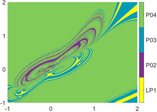
model (4) in case I. Two representative examples for k1 = 0.12 and k1 = 0.18 with (x3(0), x4(0), x5(0), x6(0)) = (0,
0, 0, 0) are shown in Figs. 6(a) and 6(b), where seven colors are used to represent different types of attractors.
Here, LP1, UP1, P02, P03, P04, P08, and CH represent lower period-1, upper period-1, period-2, period-3,
period-4, period-8, and chaos, respectively, indicating the coexisting multistable patterns. Observed from Fig.
6(a), four types of attractors are revealed when k1 = 0.12 is fixed. The orange, blue, and banded yellow regionsdominate the initial plane. In addition, the riddled basins of attraction are exhibited in a small region, implying
that the model in this case is sensitive to the initial conditions and the inconspicuous extreme events are yielded
[36, 37]. When k1 is increased to 0.18, as seen in Fig. 6(b), complex stability evolutions happen, leading to that
period-2 along with the riddled domain is embedded in period-4. As a result, the memristive HNN model
displays coexisting multistable patterns related to the initial conditions.
x3
Fig. 5 For k1 = 0.12, the phase portraits initiated by four different sets of initial conditions
x1(0) x1(0)
(a) (b)
Fig. 6 For two memristior coupling strengths, local attraction basins in the x1(0) − x2(0) initial plane a k1 = 0.12 b k1 =
0.18
3.2. Case II: Memristive HNN model with M1 and M2
Two memristors M1 and M2 used to link three neurons are taken into account in case II. Hence, the memristor
coupling strength matrix can be denoted as
k1 0 0
K k1 k2 0 (15)
0 k2 0
where, k1 and k2 are two parameters representing two different memristor coupling strengths. To investigate the
bifurcation scenarios with these two parameters, two-dimensional bifurcation diagram is plotted in the regions
k1 = [0.08, 0.18] and k2 = [−0.005, 0.065] under the determined initial conditions (−0.4, 0, 0, 0, 0, 0), as shown
in Fig. 7(a). Besides, when setting four representative values of k1 as 0.08, 011, 0.15, and 0.18, respectively,one-dimensional bifurcation diagrams are plotted with respect to k2, as shown in Fig. 7(b).
k1 = 0.08
k1 = 0.11
k1 = 0.15
k1 = 0.18
k1 k2
(a) (b)
Fig. 7 Bifurcation plots under the determined initial conditions (−0.4, 0, 0, 0, 0, 0) in case II a two-dimensional
bifurcation diagram with respect to k1 and k2 b one-dimensional bifurcation diagrams with respect to k2
As can be seen from Fig. 7(a), there exist eight types of attractors. Here the P00, P01, P02, P04, P08, P12,
P16, and CH represent the stable point, period-1, period-2, period-4, period-8, period-12, period-16, and chaos
respectively. The period-8, period-16, chaos, and period-12 are embedded in successive, resulting in the
occurrence of the marvelous bifurcation structure.
Glanced at Fig. 7(b), the phenomena of antimonotonicity appear distinctly. For fixed k1 = 0.08, when
increasing k2 in the region [−0.05, 0.065], the orbit of the memristive HNN model in case II begins with
period-1, goes into period-2 and period-4 via the forward period-doubling bifurcations, then degrades into
period-2 and period-1 via the reverse period-doubling bifurcations, and finally settle down stable point at k2 =
0.0614. When increasing k1 from 0.08 to 0.18, the period-4, period-8, period-12, and chaos bubbles are formed
respectively. Thus, the forward and reverse period-doubling bifurcation routes are obviously visible in
bifurcation processes for the model (4), which are affected by two memristor coupling strengths.
For k1 = 0.17 and k2 = 0.005 with fixed (x3(0), x4(0), x5(0), x6(0)) = (0, 0, 0, 0), Fig. 8 depicts the local
attraction basins related to the coexisting multiple patterns in case II. Here, P01, P02, P03, P05, and CH
represent the period-1, period-2, period-3, period-5, and chaos, respectively. There are five different colors
distributing in the x1(0) − x2(0) initial plane and the purple and yellow regions are relatively sparse. What’s
more, the red region is riddled and mixed in the blue region, which means that the extreme events also exist in
case II.
x2(0)
Fig. 8 For k1 = 0.17 and k2 = 0.005, local attraction basin in the x1(0) − x2(0) initial planeAccording to the aforementioned analysis, Fig. 9 shows the phase portraits under five sets of initial
conditions (0.4, 0, 0, 0, 0, 0), (−0.4, 0, 0, 0, 0, 0), (0.7, 0, 0, 0, 0, 0), (0.2, 0, 0, 0, 0, 0), and (−1, 1, 0, 0, 0, 0) for
the model (4) in case II. Five different types of attractors are triggered, including period-1, period-2, period-3,
period-5, and chaos.
x3
Fig. 9 For k1 = 0.17 and k2 = 0.005, the phase portraits initiated by five different sets of initial conditions
3.3. Case III: Memristive HNN model with M1, M2, and M3
In this case, three memristors from M1 to M3 are used to link three neurons end to end. Three memristor
coupling strengths from k1 to k3 are set as three adjusting parameters. And the matrix K can be referred to (5).
Considering the special situation in case III that memristive electromagnetic inductions between three
neurons are the same, i.e., k1 = k2 = k3 = k, thereby k is chosen as a single adjustable parameter in case III. For
this special situation, the bifurcation diagrams with respect to k are plotted in Fig. 10, where three sets of initial
conditions are set as (0.01, 0, 0, 0, 0, 0), (−0.01, 0, 0, 0, 0, 0), and (−0.07, 0, 0, 0, 0, 0), respectively. Observed
from Fig. 10, when increasing k from 0 to 0.04, the phenomena of cascaded chaotic bubbles, chaos crisis
scenarios, and coexisting bifurcations emerge in the memristive HNN model.
x3
Fig. 10 Bifurcation diagrams of x3 in case III under three sets of initial conditions
Specifically, when setting the initial conditions as (−0.07, 0, 0, 0, 0, 0), the forward and reverse
period-doubling bifurcation routes are also visible in bifurcation processes. Accordingly, when we endow four
sets of parameter k for the model (4) in case III, the phase portraits of chaotic attractor, periodic limit cycles,
and stable point are plotted in Fig. 11.x3
Fig. 11 For different k with fixed initial conditions (−0.07, 0, 0, 0, 0, 0), the phase portraits of the memristive HNN model
under the special situation of case III
In this special situation of case III, to uncover the initial-dependent dynamics, the value of k is kept as 0.005.
The local attraction basin is plotted in Fig. 12 and the coexisting tri-stable patterns are displayed, such as the
blue period-1 (P01), light cyan period-2 (P02), and red chaos (CH). Note that all the red regions are fully mixed
and riddled in the light cyan periodic regions, meaning the occurrence of the rare, recurrent, and irregular
dynamics of extreme event.
x2(0)
Fig. 12 For k = 0.005, the local attraction basin in the x1(0) − x2(0) initial plane, indicating the occurrence of the
initial-related extreme event
In summary, the dynamical effects on the memristive HNN model given in (4) are listed in Table 2. As can
be seen, when the number of memristors increases from zero to two, the number of coexisting attractors goes
from two to four and to five. However, when the memristive HNN model involves three memristors with the
aforesaid special situation, the coexisting tri-stable patterns with extreme event appear distinctly. Besides, the
anti-monotonicity behavior displays in case II, which is related to two memristor coupling strengths. Notably,
we remark that when three memristors utilized in the memristive HNN model are endowed with three different
memristor coupling strengths, some more intriguing and intricate dynamical effects need to be further
investigated.Table 2 Dynamical effects under different cases.
Cases Dimensionality Coexisting types Dynamical effects
Example 3 2 Bistability
Case I 4 4 Multistability
Case II 5 5 Antimonotonicity
Case III 6 3 Extreme event
4. PCB-based analog circuit validation
Electronic neuron circuit is nowadays regarded as an excellent artificial block to implement the VLSI
applying in neuromorphic computing [38]. It can be achieved in three ways, namely, analog, digital, and hybrid
analog/digital circuits [39–42]. In this section, the memristive HNN model is implemented in analog circuit and
the PCB-based hardware experiments are carried out to validate the memristive electromagnetic induction
effects.
4.1. Circuit synthesis for the memristive HNN model
Based on the unified memristive HNN model given in (4), an electronic neuron circuit can be implemented
and its circuit equations are described as
dv
RC dt v RW tanh(v ) RK vVM tanh(vΦ )
(16)
RC dvΦ v v
dt
M Φ
where v and vΦ are n × 1 voltage variable matrixes, and the integrating time constant τ = RC = 10 kΩ × 10 nF =
0.1 ms. In addition, for n = 3, on account of the synaptic weight matrix W, memristor coupling strength weight
K, and matrix VM in (5), three 3 × 3 resistance arrays are presented as
R R1 R R2 R R3
RW R R4 0 R R5 (17a)
R R 0
6 R R7
R Rk1 0 R Rk 3
RK R Rk1 R Rk 2 0 (17b)
0 R Rk 2 R Rk 3
vVM 1 0 0
vVM 0 vVM 2 0 (17c)
0 0 vVM 3
where RW represents the determined resistance array, RK represents the adjustable resistance array whose values
change with different cases, and vVM represents the voltage matrix of membrane potential difference. Notice
that, because the resistances are positive in the real circuit, the negative signs in (17) are adjusted by changing
the connection way of the circuit. According to (17), the resistances in RW are configured as R1 = R/3.8 =
2.6316 kΩ, R2 = R/1.9 = 5.2632 kΩ, R3 = R/0.7 = 14.2857 kΩ, R4 = R/2.8 = 3.5714 kΩ, R5 = R/1 = 10 kΩ, R6 =
R/6.6 = 1.5152 kΩ, and R7 = R/1.3 = 7.6923 kΩ, respectively.
Circuit schematic is designed synthetically using Multisim 12.0 software, the screenshot of which can beseen in Fig. 13, where three cases of circuit modules can be controlled by six-pin DIP switch with S1 ~ S3 keys.
Therefore, the states of these three keys for the electronic neuron circuit and theoretical resistances for RK are
summarized in Table 3. Besides, three different functional circuits denoted by fourteen hierarchical blocks
(HBs) are shown in Fig. 13, where six HBs from ‘−T1’ to ‘−T6’ represent the hyperbolic tangent function
circuit modules with negative output, five HBs from ‘−H1’ to ‘−H5’ represent the inverting operation circuits,
and three HBs from ‘I1’ to ‘I3’ represent the subtraction operation circuits. Notice that, global connectors are
employed to connect the common port for simplifying the circuital connection.
Memristor 1
Memristor 2
Memristor 3
Circuit module for the memristive HNN Circuit modules for three memristors
Fig. 13 Schematic diagram for implementing the memristive HNN model given in (16)
Table 3 Four cases of circuit modules controlled by a DIP switch and theoretical resistances for RW and RK.
S1 S2 S3 Cases of memristive HNN model Theoretical resistances in RW and RK
off off off An example of the HNN model RW = R/|wij|, W = 1,…,7
on off off Case I: Memristive HNN model with M1 Rk1 = R/k1 = 83.33 kΩ
on on off Case II: Memristive HNN model with M1 and M2 Rk1 = R/k1 = 58.82 kΩ, Rk2 = R/k2 = 2000 kΩ
on on on Case III: Memristive HNN model with three M Rk = R/k = 2MΩ, 500 kΩ, 333.33 kΩ, and 250 kΩ
4.2. PCB-based hardware circuit validation
The designed PCB is made using the Altium designer 10.0 software. The off-the-shelf commercial
components contain bipolar junction transistor MPS2222, operational amplifier TL082CP, operational amplifier
AD633JNZ, chip resistor, precision potentiometer, and monolithic ceramic capacitor. And the phase portraits
are captured by Tektronix digital oscilloscope in the X-Y mode.
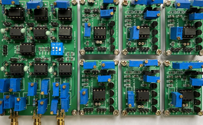
The photograph of the electronic neuron circuit is displayed in Fig. 14, where the HNN circuit module is in
the left, and six same and independent −tanh(ꞏ) modules are in the right dotted box. ‘S’ is a six-pin DIP switch
that is used to control the circuit connection states. For instance, when S1 and S2 are on and S3 is off in thisfigure, the circuit is in the state of case II.
Fig. 14 PCB-based electronic neuron circuit for implementing the memristive HNN model
On account of Table 3, when three keys are all off, the example of the HNN model given in (1) can be
denoted by a third-order analog circuit. Besides, when case I and case II are classified, the adjustable resistance
arrays RK are configured as
R Rk1 0 0
RK R Rk1 0 0 (18a)
0 0 0
R Rk1 0 0
RK R Rk1 R Rk 2 0 (18b)
0 R Rk 2 0
respectively, where Rk1 and Rk2 are two adjustable resistances for each case. When configuring the two
resistances in turn, the phase portraits for the first two cases are experimentally captured, as shown in Fig. 15.
Note that due to the difficulty in achieving specific capacitor initial voltages in analog circuit, power supply
should be on-and-off switched to endow the initial conditions in the real circuit [31, 43]. In Fig. 15, three types
of attractors coexisted in case I and three types of attractors coexisted in case II can be captured. And the
initial-related coexisting behaviors can be availably realized by circuit simulations [27, 30].
v3, 1V/div
v3, 1.25V/div
Fig. 15 The phase portraits captured by adjusting the states of keys and the resistances RK a experimental resistance Rk1 =
83.33 kΩ in case I b experimental resistances Rk1 = 58.82 kΩ and Rk2 = 2012 kΩ in case II
Furthermore, when three keys are all on, the adjustable resistance array RK is configured as (17b). For the
special situation in case III, the adjustable resistances need to be the same, i.e., Rk = Rk1 = Rk2 = Rk3 = R/k1 = R/k2
= R/k3. Thus, the experimental phase portraits can be captured and shown in Fig. 16. As can be seen, dynamicalevolutions from chaos to period-2, to period-1, and to stable point can be readily observed and the experimental
results validate the simulation results given in (11). Besides, the photograph of PCB-based hardware circuit for
case III is shown in Fig. 16(b), in which the chaotic attractor is cropped by Tektronix digital oscilloscope.
v3, 1V/div
Fig. 16 When S1 ~ S3 are all on, experimental phase portraits and photograph a four captured phase portraits by setting Rk1
= Rk2 = Rk3 = 2000 kΩ, 600 kΩ, 430 kΩ, and 250 kΩ, respectively b photograph for PCB-based hardware circuit linked with
a digital oscilloscope
Due to the parasitic resistances and inner interferences in the real circuit, PCB-based experiment results are
consistent with the numerical results basically though possessing some errors. In general, we can say that the
electronic neuron circuit for implementing the memristive HNN model well validates the memristive
electromagnetic induction effects on HNN. And in the next step, we may try to use simple activation function
in HNN, or find some alternative schemes for the complex activation functions so as to investigate the unified
HNN model with n neurons.
5. Conclusions
Using the threshold hyperbolic-type memristors to link the interconnected neurons, this paper presented a
unified memristive HNN model to simulate electromagnetic induction effects. The uniform boundedness of the
unified memristive HNN model was deduced in theory, proving that all the motions are trapped into a bounded
region. With the consideration of three cases, the dynamical effects were revealed in succession using multifold
dynamical analysis methods. In case I, stability analysis proved that the equilibrium points are all unstable
saddle-foci, and numerical simulations disclosed the coexisting bifurcation behaviors and coexisting
multistable patterns herein. In case II, the antimonotonicity phenomena appeared with the creation and
annihilate of periodic and chaotic bubbles, which was controlled by two memristor coupling strengths. Besides,
coexisting five-stable patterns were induced by the initial conditions. In the special situation of case III, when
three memristor coupling strengths were the same, the extreme event with complex riddled basins taken place
distinctly, meaning that the memristive HNN model is increasingly sensitive to the initial conditions.
The electronic neuron circuit of the memristive HNN model was constructed by a PCB hardware platform,
and the results beautifully validated the numerical simulations for three cases. Accordingly, the study of the
memristive electromagnetic induction effects on HNN not only reveals the interactions of neurons, but also
provides a potential application in the neuromorphic computation. Furthermore, we emphasize that, based on
the other examples of memristive HNN models, the electromagnetic induction effects may not the same and
need to be explored in the future.Acknowledgements
This work was supported by the National Natural Science Foundation of China under Grant Nos. 61971228
and 51777016, the Natural Science Foundation of Henan Province under Grant No. 202300410351, and the
Key Scientific Research of Colleges and Universities in Henan Province under Grant No. 21A120007.
Compliance with ethical standards
Conflict of interest The authors declare that they have no conflicts of interest. These authors contribute
equally to this work.
Availability of data and materials
The datasets supporting the conclusions of this article are included within the article and its additional files.
References
1. Chua, L.O.: Memristor-The missing circuit element. IEEE Trans. Circuit Theory 18(5), 507−519 (1971)
2. Kumar, S., Strachan, J., Williams, R.: Chaotic dynamics in nanoscale NbO2 Mott memristors for analogue computing.
Nature 548, 318−321 (2017)
3. Li, C., Min, F.H., Li, C.B.: Multiple coexisting attractors of the serial-parallel memristor-based chaotic system and its
adaptive generalized synchronization. Nonlinear Dyn. 94, 2785−2806 (2018)
4. Xie, W.L., Wang, C.H., Lin, H.R.: A fractional-order multistable locally active memristor and its chaotic system with
transient transition, state jump. Nonlinear Dyn. 104, 4523−4541 (2021)
5. Miranda, E., Milano, G., Ricciardi, C.: Modeling of short-term synaptic plasticity effects in ZnO nanowire-based
memristors using a potentiation-depression rate balance equation. IEEE Trans. Nanotechnol. 19, 609−612 (2020)
6. Lv, M., Wang, C.N., Ren, G.D., Ma, J., Song, X.L.: Model of electrical activity in a neuron under magnetic flow effect.
Nonlinear Dyn. 85(3), 1479−1490 (2016)
7. Bao, H., Chen, C.J., Hu, Y.H., Chen, M., Bao, B.C.: Two-dimensional piecewise-linear neuron model. IEEE Trans.
Circuits Syst. II, Exp. Briefs 68(4), 1453−1457 (2021)
8. Xu, Y., Jia, Y., Ma, J., Alsaedi, A., Ahmad, B.: Synchronization between neurons coupled by memristor. Chaos Solit.
Fractals 104, 435−442 (2017)
9. Sun, J.W, Xiao, X., Yang, Q.F., Liu, P., Wang, Y.F.: Memristor-based Hopfield network circuit for recognition and
sequencing application. AEÜ-Int. J. Electron. Commun. 134, 153698 (2021)
10. Hong, Q.H., Yan, R., Wang, C.H, Sun, J.R.: Memristive circuit implementation of biological nonassociative learning
mechanism and its applications. IEEE Trans. Biomedical Circuits Syst. 14(5), 1036−1050 (2020)
11. Ma, J., Tang, J.: A review for dynamics in neuron and neuronal network. Nonlinear Dyn. 89(3), 1569−1578 (2017)
12. Ge, M.Y., Jia, Y., Xu, Y., Yang, L.J.: Mode transition in electrical activities of neuron driven by high and low frequency
stimulus in the presence of electromagnetic induction and radiation. Nonlinear Dyn. 91(1), 515−523 (2017)
13. Parastesh, F., Azarnoush, H., Jafari, S., Hatef, B., Perc, M., Repnik, R.: Synchronizability of two neurons with
switching in the coupling. Appl. Math. Comput. 350, 217−223 (2019)
14. Fang, T.T., Zhang, J.Q., Huang, S.F., Xu, F., Wang, M.S., Yang, H.: Synchronous behavior among different regions of
the neural system induced by electromagnetic radiation. Nonlinear Dyn. 98(17), 1267−1274 (2019)
15. Parastesh, F., Rajagopal, K., Alsaadi, F.E., Hayat, T., Pham, V.T., Hussain, I.: Birth and death of spiral waves in a
network of Hindmarsh-Rose neurons with exponential magnetic flux and excitable media. Appl. Math. Comput. 354,
377−384 (2019)
16. Takembo, C.N., Mvogo, A., Fouda, H.P.E., Kofané, T.C.: Effect of electromagnetic radiation on the dynamics of
spatiotemporal patterns in memristor-based neuronal network. Nonlinear Dyn. 95, 1067−1078 (2018)
17. Bao, H., Hu, A.H., Liu, W.B., Bao, B.C.: Hidden bursting firings and bifurcation mechanisms in memristive neuron
model with threshold electromagnetic induction. IEEE Trans. Neural Netw. Learn. Syst. 31(2), 502−511 (2020)
18. Bao, H., Liu, W.B., Hu, A.H.: Coexisting multiple firing patterns in two adjacent neurons coupled by memristive
electromagnetic induction. Nonlinear Dyn. 95, 43−56 (2019)
19. Li, R.H., Wang, Z.H., Dong, E.Z.: A new locally active memristive synapse-coupled neuron model. Nonlinear Dyn. 104,
4459−4475 (2021)
20. Ma, J., Yang, Z.Q., Yang, L.J., Tang, J.: A physical view of computational neurodynamics. J. Zhejiang Univ. Sci. A20(9), 639−659 (2019)
21. Zhou, Q., Wei, D.Q.: Collective dynamics of neuronal network under synapse and field coupling. Nonlinear
Dyn. (2021). https://doi.org/10.1007/s11071-021-06575-0
22. Yang, K., Duan, Q.X., Wang, Y.H., Zhang, T., Yang, Y.C., Huang, R.: Transiently chaotic simulated annealing based on
intrinsic nonlinearity of memristors for efficient solution of optimization problems. Sci. Adv. 6(33), eaba9901 (2020)
23. Pu, Y., Yi, Z., Zhou, J.: Fractional Hopfield neural networks: Fractional dynamic associative recurrent neural networks.
IEEE Trans. Neural Netw. Learn. Syst. 28(10), 2319−2333 (2017)
24. Cai, F.X., Kumar, Suhas., Vaerenbergh, T.V., et al.: Power-efficient combinatorial optimization using intrinsic noise in
memristor Hopfield neural networks. Nat. Electron. 3(7), 409−418 (2020)
25. Wang, Z., Parastesh, F., Rajagopal, K., Hamarash, I.I., Hussain, I.: Delay-induced synchronization in two coupled
chaotic memristive Hopfield neural networks. Chaos Solit. Fractals 134, 109702 (2020)
26. Pham, T., Jafari, S., Vaidyanathan, S., Volos, C., Wang. X.: A novel memristive neural network with hidden attractors
and its circuitry implementation. Sci. China Tech Sci. 59(3), 358−363 (2016)
27. Lin, H.R., Wang. C.H., Hong, Q.H., Sun, Y.C.: A multi-stable memristor and its application in a neural network. IEEE
Trans. Circuits Syst. II, Exp. Briefs 67(12), 3472−3476 (2020)
28. Hu, X.Y., Liu, C.X., Liu, L., Ni, J.K., Yao, Y.P.: Chaotic dynamics in a neural network under electromagnetic radiation.
Nonlinear Dyn. 91, 1541−1554 (2018)
29. Lin, H.R., Wang, C.H., Tan, Y.M.: Hidden extreme multistability with hyperchaos and transient chaos in a Hopfield
neural network affected by electromagnetic radiation. Nonlinear Dyn. 99, 2369−2386 (2020)
30. Chen, C.J., Chen, J.Q., Bao, H., Chen, M., Bao, B.C.: Coexisting multi-stable patterns in memristor synapse-coupled
Hopfield neural network with two neurons. Nonlinear Dyn. 95(4), 3385−3399 (2019)
31. Chen, C.J., Bao, H., Chen, M., Xu, Q., Bao, B.C.: Non-ideal memristor synapse-coupled bi-neuron Hopfield neural
network: Numerical simulations and breadboard experiments. AEÜ-Int. J. Electron. Commun. 111, 152894 (2019)
32. Zheng, P.S., Tang, W.S., Zhang, J.X.: Dynamic analysis of unstable Hopfield networks. Nonlinear Dyn. 61(3), 399−406
(2010)
33. Khalil, H. K.: Nonlinear systems, Third edition. Upper Saddle River, NJ, USA: Prentice-Hall, 2002
34. Chen, T.P., Amari, S. I.: Stability of asymmetric Hopfield networks. IEEE Trans. Neural Netw. Learn. Syst. 12(1),
159−163 (2001)
35. Silva, C.P.: Shil’nikov’s theorem-a tutorial. IEEE Trans. Circuits Syst. I, Fundam. Theory Appl. 40(10), 675−682 (1993)
36. Saha, A., Feudel, U.: Riddled basins of attraction in systems exhibiting extreme events. Chaos 28(3), 033610 (2018)
37. Wang, G.Y., Yuan, F., Chen, G.R., Zhang, Y.: Coexisting multiple attractors and riddled basins of a memristive system.
Chaos 28(1), 013125 (2018)
38. Ribar, L., Sepulchre, R.: Neuromodulation of neuromorphic circuits. IEEE Trans. Circuits Syst. I, Reg. Papers 66(8),
3028−3040 (2019)
39. Haghiri, S., Naderi, A., Ghanbari, B., Ahmadi, A.: High speed and low digital resources implementation of
Hodgkin-Huxley neuronal model using base-2 functions. IEEE Trans. Circuits Syst. I, Reg. Papers 68(1), 275−287 2021
40. Jokar, E., Abolfathi, H., Ahmadi, A., Ahmadi, M.: An efficient uniform-segmented neuron model for large-scale
neuromorphic circuit design: Simulation and FPGA synthesis results. IEEE Trans. Circuits Syst. I, Reg. Papers 66(6),
2336−2349 (2019)
41. Li, K.X., Bao, H., Li, H.Z., Ma, J., Hua, Z.Y., Bao, B.C.: Memristive Rulkov neuron model with magnetic induction
effects. IEEE Trans. Ind. Informat. (2021). https://doi.org/10.1109/TII.2021.3086819
42. Lin, H.R., Wang, C.H., Chen, C.J., Sun, Y.C., Zhou, C., Xu, C., Hong, Q.H.: Neural bursting and synchronization
emulated by neural networks and circuits. IEEE Trans. Circuits Syst. I, Reg. Papers (2021).
https://doi.org/10.1109/TCSI.2021.3081150
43. Bao, B.C., Jiang, T., Wang, G.Y., Jin P.P., Bao, H., Chen, M.: Two-memristor-based Chua’s hyperchaotic circuit with
plane equilibrium and its extreme multistability. Nonlinear Dyn. 89(2), 1157−1171 (2017)You can also read