Carroll Collected John Carroll University

John Carroll University
Carroll Collected

Senior Honors Projects                                                        Honor's Program

2023

Time Series Forecasting for Stock Market Prices
Albert Zhou

Follow this and additional works at: https://collected.jcu.edu/honorspapers

   Part of the Computer Sciences Commons, and the Data Science Commons

Albert Zhou

Elena Manilich

DATA 470

15 December 2022

                         Time Series Forecasting for Stock Market Prices

INTRODUCTION

       The stock market has attracted customers over the years with its built-in high risk and

high reward system. With an endless increase in market capitalization, stock trading has become

the center of investment for many investors. The savings and investments that the system can

potentially generate have vitalized the continuously growing national economy. However, this

system has proven to be dynamic and complex, which supplies to the risk factor involved. In

order to reduce risk, experienced investors have found it advantageous to use technology that

predicts future stock prices.

       A classic approach to Stock Market Prediction (SMP) includes fundamental and technical

analysis, but a more modern approach includes machine learning and sentiment analysis. In this

paper, time series forecasting for SMP will be explored. The Auto-Regressive Integrated Moving

Average (ARIMA), which is a classical statistical method, will be the primary method and

described in detail. The Long-Short Term Memory (LSTM) method, which is under deep

machine learning, will be the secondary method and described briefly. The stock market price

time series data that expands over six years for a group of high tech companies will be used and

prediction of each stock price will be presented by both ARIMA and LSTM models.

       ARIMA is a statistical analysis model that uses time series data to either better

understand the data set or to determine future trends, predicting future values based on past

values. For example, an ARIMA model might seek to predict a stock's future prices based on its

past performance or forecast the earnings of a company based on past periods. The LSTM model

is a powerful recurrent neural network (RNN) approach that has been used to achieve the

best-known results for many problems on sequential data. LSTM cells are used in recurrent

neural networks to predict future values from sequences of variable lengths. Recurrent neural

networks work with any kind of sequential data and, unlike ARIMA and Prophet, are not

restricted to time series data. The main idea behind LSTM is to learn the important parts of the

sequence seen so far and disregard the parts that are not as significant. This is achieved by the

so-called functions that have different learning objectives such as representing the time series in

a compact manner, combining the past representation of the series with new inputs, forgetting the

insignificant parts of the series while generating a prediction for the next time step.

DATA

       Our data was sourced from Yahoo Finance, a public domain that provides financial news,

data, and commentary updated in real time. Originating from the United States Securities and

Exchange Commision (SEC), the data supports over 40,000 stock quotes across multiple

exchange markets and is provided in statement categories such as income, balance, and cashflow.

For this paper, we will target the historical price data pertaining to certain stocks we have

hand-picked in order to predict the future values of those stocks.

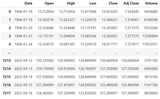
       Our data contains the daily historical price data over the past 28 years, from 1994 to

2022. Data for each individual stock quote is downloaded as a dataframe, which provides 1) the

daily opening price of the stock (Open), 2) the daily maximum price of the stock (High), 3) the

daily minimum price of the stock (Low), 4) the daily closing price of the stock (Close), 5) the

daily adjusted closing price (Adj Close), and 6) the daily total number of shares traded (Volume).

Figure 1: IBM Closing Price Data from 1994-2022

Figure 2: Head of IBM Historical Price Data

ANALYTICAL METHODS - ARIMA MODEL AND RESULTS

       We want to construct a model that can investigate patterns in the stock market by

reviewing the trends constructed from the data we collected and concatenated. The ARIMA

model uses time series data to predict future points in the series (also known as time-series

forecasting).

       There are three integers that are typically used to parametrize nonseasonal ARIMA

models. They are p, the number of autoregressive terms (AR order), d, the number of

nonseasonal differences (differencing order), and q, the number of moving-average terms (MA

order). One method to select these values for the ARIMA model is by using the auto_arima

function from the pmdarima package. This machine learning approach chooses values in such a

way that the Akaike Information Criterion (AIC) score is minimized. We can store this model as

a variable for future reference. Another method that is more complex and subjective involves

differencing the data to determine the d parameter and then generating autocorrelation (ACF) and

partial autocorrelation (PACF) plots to determine the q and p parameters, respectively. We will

explore this method shortly.

       The ARIMA model, among other models such as linear regression, assumes that the data

is stationary, meaning that the data and its variance should not be a function of time. In other

words, the dependent values of an observation should not depend on when it is observed. By

removing any obvious correlation and collinearity within past data, we can ensure that the data

will have the same behavior at some later point in time and is therefore predictable. We can

determine whether or not our data is stationary by running an Augmented Dicky-Fuller (ADF)

Test from the statsmodels package. For instance, we ran the test on the daily closing price for our

selected stocks. Since the p-value in each output was far greater than the threshold of 0.05, we

cannot reject the null hypothesis of the test, which concludes the data is nonstationary. We would

expect this data to be nonstationary as stock prices have naturally changed over time, and there

would be no trend to predict if this was not the case. If we were to continue using this data

without transformation, we would most likely run into bias within our results. A simple method

to make the data stationary involves taking the log of one of the dependent variables (we

performed this operation on the daily adjusted closing price of the stock). This lowers the rate at

which the dependent variable changes, removing any signs of correlations within the data.

Another method which is more necessary for determining the ARIMA parameters is differencing

the data. This involves taking the difference between the dependent values of the two data points

adjacent to each point. This value then becomes the new value of the dependent variable. We can

graph these new values as “first-order differencing.” Differencing can be iterated on the same

data multiple times if necessary, which would allow plots for “second-order differencing,”

“third-order differencing,” and so on.

       When the ADF test was run again after first-order differencing, the p-value was slightly

below 0.05, indicating the time series had become more stationary than with the original data.

The stationary nature could be further enhanced by applying second-order differencing. We

could further confirm that our data is stationary by plotting the rolling mean and standard

deviation. This meant taking the mean of the dependent values of a certain number of data points

before each point and recording this mean as the new dependent value (shown in Figure 3). After

second-order differencing was applied, the ADF test generated p-values well below 0.05 for each

of the stocks. Therefore, we were safe to assume that this data was now stationary and that a

value of 2 for the d parameter was acceptable for each stock. There were other methods that

could be implemented to make the data stationary, and although they made the data more

stationary than the original, they performed worse than taking the log of the dependent variable

and then differencing.

Figure 3: Rolling Mean and Standard Dev. of the Transformed Data for TSLA

        Once a time series has been made stationary by differencing, we will need to split the

data into training and testing datasets. The training dataset will be used to prepare the ARIMA

model and generate a prediction. The testing dataset, which is much smaller than the training

dataset, will be the part of the data that we will try to predict. The size of our testing dataset, with

dates ranging from October 2020 to February 2021, is about 7 percent of the size of our training

dataset, which ranges back to the beginning of 2015 (shown below).

Figure 4: The Train and Test Data for TSLA

        The next step in fitting the ARIMA model is to determine the p and q parameters. Of

course, we could use the auto_arima function that was discussed earlier to determine these

values, or we could also test various combinations of p and q values and see what works best.

However, observing the autocorrelation function (ACF) and partial autocorrelation (PACF) plots

is probably the most systematic (if not accurate) method. With these plots generated from the

statsmodels package, we can tentatively identify the values of AR and/or MA terms that are

needed. They calculate the mean correlation between points that are a certain number of lags

apart, with the number of lags being the independent variable. A lag refers to the time period

between each point in the original data, with two adjacent points being one lag apart, for

example.

       Shown in Figures 5-6, Both the ACF and PACF plots start at a lag value of 0, which

always has a correlation value (the dependent variable) of 1. This is because we are essentially

calculating the correlation between identical points at this stage. With a lag value of 1, we can

determine the relation between adjacent observations and whether or not this relation is

significant. The ACF and PACF plots can differ starting at the lag value of 2. This is because the

ACF takes into account indirect correlations from previous lags in the calculation. The PACF,

meanwhile, does not consider the common correlation involving data points that are between the

points being evaluated (lower-order lags). Therefore, the PACF is expected to decay much faster.

A region that depicts the 95% confidence interval for correlation is displayed within each plot.

Correlation values are deemed statistically close to zero if they fall inside this region. Whether or

not certain points fall within the confidence interval will determine our prediction for the p and q

parameters.

       The PACF plot is used to estimate the p parameter. We can take the order of the AR term

to be equal to the number of a lag that is outside the 95% confidence interval. By selecting a lag

in this manner, we are implying that the selected lag explains the autocorrelations of all lags of a

higher order (number), most of which we are assuming are within the confidence interval. We

can do the same for the ACF plot to estimate the q parameter and take the order of the MA term.

Figures 5A-B: ACF and PACF plots of Transformed Data for TSLA Before Differencing

Figures 6A-B: ACF and PACF plots of Transformed Data for TSLA After 2nd Order
Differencing

       The ARIMA model can be constructed with the p, d, and q parameters that were

determined by the auto_arima function or with the ACF and PACF plots. Going back to

auto_arima, the function outputs the ARIMA model with the parameters that minimize the

Akaike Information Criterion (AIC) score. We can feed these parameters along with our data into

the ARIMA function from the statsmodels package, which will return a trained model used for

evaluation and inference. This process can be repeated with the parameters determined by the

ACF and PACF plots, or for the sake of experimentation and adjusting the AIC score, parameters

of our own choosing as long as they are positive integers. The model summary accepts and

displays the parameters in the form ( p, d, q ) and will provide several measures that can evaluate

the performance of the model. A number of coefficient values equal to the value of the p and q

parameters are also provided for each. For instance, if the value of the p parameter was 2, there

would be two coefficient values provided in the model for that parameter, as shown in Fig. 7.

Figure 7: Example of ARIMA Model Output for TSLA

       These coefficients are taken into account when the forecast() function from the

statsmodels package is run. This function generates predictions for the dependent variable for the

timespan of the test data. The output is stored as a series of values which we can convert into a

two-column pandas dataframe. We can plot our predictions along with the train and test data to

compare them visually, reverting any transformations done on the data if necessary by applying

the inverse of those transformations. Once the train, test, and predictions data have been plotted

together on the correct scale, we can calculate the root mean squared error (RMSE) of the

prediction data and repeat this process for other combinations of the p, d, and q parameters. A

smaller RMSE indicates that the prediction data aligns better with the test data, therefore we will

want to compare RMSE values associated with various parameter combinations, including the

ones calculated by the auto_arima function as well as the ACF and PACF plots.

Figure 8A: TSLA Model Prediction with Parameters (5, 2, 2)

       We can objectively compare the results taken from our prediction dataframe with the

original test data. From the example in Figure 8A (in which the prediction data used the

parameters suggested by the auto_arima function), we can observe that the prediction data

follows the overall trend of the test data. The root mean square error (RMSE) provided by this

prediction data was determined to be 102.60. When using the parameters suggested by the ACF

and PACF plots instead, the prediction data also followed a positive trend. However, some of the

predicted values strayed beyond the range of the dependent values of the test data. Furthermore,

the RMSE of this data was calculated to be greater than the previously mentioned RMSE.

Therefore, we can conclude that the auto_arima function offers a better model prediction for the

Tesla (TSLA) stock. In this case, the prediction was accurate enough to the point that further

experimentation with combinations of parameters was not necessary. This would be done with

data involving other stocks where the model predictions offered by both of the two previously

discussed methods were inadequate.

       The similar practices are performed to the stock price data of APPLE, Google, Microsoft,

Amazon, Gamestop, Costco, GE and the corresponding best results are shown in Figs. 8B-8H.

Figure 8B: APPL Model Prediction with Parameters (2, 2, 2)

Figure 8C: GOOG Model Prediction with Parameters (2, 2, 0)

Figure 8D: MSFT Model Prediction with Parameters (2, 2, 2)

Figure 8E: AMZN Model Prediction with Parameters (0, 1, 0)

Figure 8F: GME Model Prediction with Parameters (5, 2, 2)

Figure 8G: COST Model Prediction with Parameters (2, 2, 2)

Figure 8H: GE Model Prediction with Parameters (2, 2, 0)

ANALYTICAL METHODS - LSTM MODEL AND RESULTS

       The LSTM model is an artificial Recurrent Neural Network (RNN) used in deep learning

that can process entire sequences of data. The model has become a trending approach to time

series forecasting. RNNs typically have short term memory, persistently using previous

information in the current neural network. They can frequently experience a loss of information

due to the repeated use of the Recurrent Weight Matrix (RWM). This is sometimes referred to as

the “Vanishing Gradient Problem.”

Other time series forecasting models can predict future values based on previous,

sequential data using the LSTM model. This provides greater accuracy for demand forecasters

which can result in better decision making for the business. The model provides nonlinear

forecasts but requires more computation than other RNNs. This is mainly due to the additional

parameters used for demand forecasts. Advanced theory on the LSTM model will not be

provided in this study. We have instead described the major steps of the modeling process and

visually presented the model results (shown below). The model generates a prediction over the

test data in a similar manner to the ARIMA model. The corresponding results are shown in Figs.

9A-9H, which provided much more details of the trend of the stock price.

Figure 9A: TSLA LSTM Model Prediction

Figure 9B: AAPL LSTM Model Prediction

Figure 9C: GOOG LSTM Model Prediction

Figure 9D: MSFT LSTM Model Prediction

Figure 9E: AMZN LSTM Model Prediction

Figure 9F: GME LSTM Model Prediction

Figure 9G: COST LSTM Model Prediction

Figure 9H: GE LSTM Model Prediction

DISCUSSION

       In summary, the ARIMA model is a statistical technique that can be used to forecast time

series data. It is a linear model. The LSTM could predict the nonlinear relationship for

forecasting. It can predict the trend more accurately. The RMSE results for eight stocks are

summarized in Table 1 from both ARIMA and LSTM models. However the LSTM approach

requires more computation than other recurrent neural networks. The main reason is that it has

more parameters, which are used for demand forecasts. Both techniques can be effective and

valuable to investigate trends in stock market prices over large periods of time and provide some

important information for investors to make decisions when investing in the stock market.

Table I: The Root Mean Square Errors (RMSEs) for Model Predictions

Stock                           RMSE (ARIMA)                RMSE (LSTM)

TSLA                                 102.60                     65.14

APPL                                  5.40                      4.69

GOOG                                 80.69                      70.76

MSFT                                  7.32                      5.87

AMZN                                 105.70                    154.76

GME                                  14.59                      14.05

COST                                 16.44                      8.44

GE                                   11.17                      5.21

References

Agarwal, Divyant. “Time Series Part 3 - Stock Price Prediction Using ARIMA Model with

       Python.” LinkedIn, 14 May 2022.

Angadi, Mahantesh C., and Amogh P. Kulkarni. "Time Series Data Analysis for Stock Market

       Prediction using Data Mining Techniques with R." International Journal of Advanced

       Research in Computer Science, vol. 6, no. 6, 2015.

Brownlee, Jason. “How to Make Out-of-Sample Forecasts with ARIMA in Python.” Machine

       Learning Mastery, 24 Mar. 2017.

Drelczuk, Krzysztof. “ACF (Autocorrelation Function) - Simple Explanation with Python

       Example.” Medium, 7 May 2020.

Gamboa, John Cristian Borges. "Deep Learning for Time-Series Analysis." arXiv, 7 Jan. 2017.

Kannan, K. Senthamarai, et al. "Financial stock market forecast using data mining techniques."

       Proceedings of the International Multiconference of Engineers and Computer Scientists,

       vol. 1, 2010.

Khedr, Ayman E., and Nagwa Yaseen. "Predicting Stock Market Behavior Using Data Mining

       Technique(s) and News Sentiment Analysis." International Journal of Intelligent Systems

       and Applications, vol. 9, no. 7, 2017.

Kutzkov, Konstantin. “ARIMA vs Prophet vs LSTM for Time Series Prediction.” MLOps Blog,

       14 Nov. 2022.

Lianne, Justin. “How to Build ARIMA Models in Python for Time Series Prediction.” Just into

       Data, 25 Aug. 2022.

Malkin, Cory. “ARIMA Model Python Example - Time Series Forecasting.” Towards Data

       Science, 25 May 2019.

Montenegro, Carlos, and Marco Molina. "Improving the Criteria of the Investment on Stock

       Market Using Data Mining Techniques: The Case of S & P 500 Index." International

       Journal of Machine Learning and Computing, vol. 10, no. 2, 2020, pp. 309-315.

Prabhakaran, Selva. “ARIMA Model - Complete Guide to Time Series Forecasting in Python.”

       Machine Learning +, 22 Aug. 2021.

Vaidya, Ajinkya M., Nikunjkumar H. Waghela, and Sneha S. Yewale. "Decision Support System

       for the Stock Market Using Data Analytics and Artificial Intelligence." International

       Journal of Computer Applications, vol. 117, no. 8, 2015.

Zvornicanin, Enes. “Choosing the Best q and p from ACF and PACF Plots in ARMA-type

       Modeling.” Baeldung, 8 Nov. 2022.