How fast could Usain Bolt have run? A dynamical study
←
→
Page content transcription
If your browser does not render page correctly, please read the page content below
How fast could Usain Bolt have run? A dynamical study
H. K. Eriksena兲
Institute of Theoretical Astrophysics, University of Oslo, P.O. Box 1029 Blindern, N-0315 Oslo, Norway
and Centre of Mathematics for Applications, University of Oslo, P.O. Box 1053 Blindern,
N-0316 Oslo, Norway
J. R. Kristiansenb兲 and Ø. Langangenc兲
Institute of Theoretical Astrophysics, University of Oslo, P.O. Box 1029 Blindern, N-0315 Oslo, Norway
I. K. Wehusd兲
Department of Physics, University of Oslo, P.O. Box 1048 Blindern, N-0316 Oslo, Norway
共Received 1 September 2008; accepted 3 November 2008兲
Since that memorable day at the Beijing 2008 Olympics, a big question has been, “What would the
100 m dash world record have been had Usain Bolt not celebrated at the end of his race?” Bolt’s
coach suggested that the time could have been 9.52 s or better. We consider this question by
measuring Bolt’s position as a function of time using footage of the run, and then extrapolate the last
2 s with two different assumptions. First, we conservatively assume that Bolt could have maintained
the runner-up’s acceleration during the end of the race. Second, based on the race development prior
to the celebration, we assume that Bolt could have kept an acceleration of 0.5 m / s2 greater than the
runner-up. We find that the new world record in these two cases would have been 9.61⫾ 0.04 and
9.55⫾ 0.04 s, respectively, where the uncertainties denote 95% statistical errors. © 2009 American
Association of Physics Teachers.
关DOI: 10.1119/1.3033168兴
I. INTRODUCTION these videos, we printed ⬇30 screen shots at different times,
from which we estimate the runners’ positions as a function
On Saturday, 16 August 2008, Usain Bolt shattered the of time.
world record of the 100 m dash at the Beijing Olympics This task is made considerably easier by the presence of a
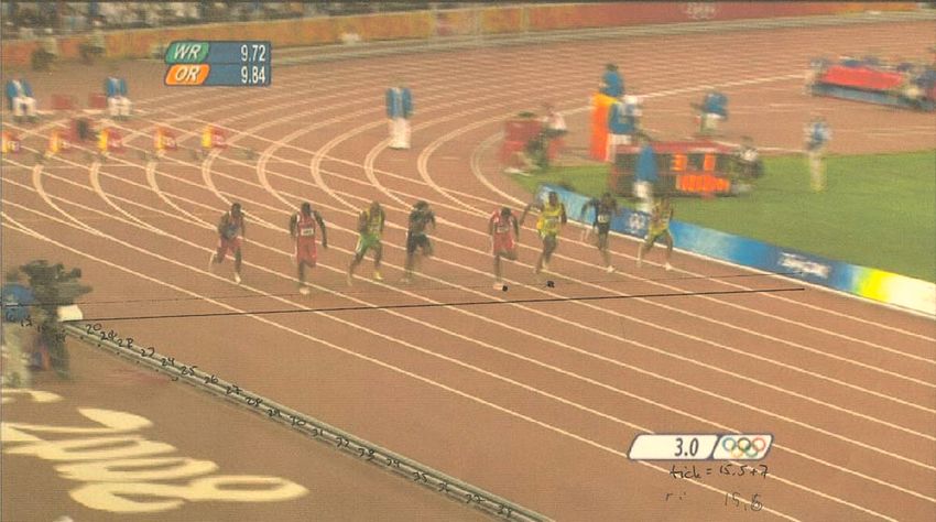
2008. In a spectacular run dubbed, “the greatest 100 meter moving camera mounted to a rail along the track 共see Fig. 1兲.
performance in the history of the event” by Michael Johnson, This rail is bolted to the ground at regular intervals, and
Bolt finished at 9.69 s, improving his own previous world thereby provides the required standard ruler. We then cali-
record set earlier in 2008 by 0.03 s. However, the most im- brated this standard ruler by counting the total number of
pressive fact about his new world record was the way in
bolts 共called “ticks” in the following兲 on the rail of the mov-
which he did it. After accelerating away from the rest of the
ing camera along the 100 m track 共see Fig. 1兲. We assumed
field, he looked to his sides when 2 s and 20 m remained and
started celebrating! He extended his arms, and appeared to the distance between the ticks to be constant.
almost dance along the track. This celebration left spectators Next, we drew lines orthogonal to the track, using what-
and commentators wondering, “What would the world ever means was most accurate for a given screen shot. For
record have been had he not celebrated the last 20 m?” the early and late frames, lines in the actual track 共for ex-
Bolt’s coach, Glen Mills, later suggested that the record ample, starting and finishing lines兲 were most useful; for
could have been 9.52 s, or even better. some intermediate frames the lower front edge of the camera
In this paper we check this suggestion by measuring Bolt’s mount was utilized 共see Fig. 1兲. When reliable parallel lines
position as a function of time and extrapolate from his dy- were available, we used the method illustrated in Fig. 2 to
namics before his celebration to the last 2 s of the race. estimate positions. We first found the vanishing point in the
Based on reasonable assumptions, we obtain an estimate of horizon where two known parallel lines appear to converge
what the new world record could have been. 共that is, point P in the horizon in Fig. 2兲. Then, we drew a set
Earlier work on similar topics have typically revolved of auxiliary parallel lines from this point onto the track.
around the construction of a dynamical model of the 100 and These lines were then propagated to earlier or later frames
200 m dashes.1–3 In our work we employ strictly empirical using fixed features in the pictures.
data, and fit a nonparametric model to the observations. For a given frame we then read off the positions of Usain
Compared to the dynamical approaches, our analysis mini- Bolt and Richard Thompson, the runner-up, with the ruler,
mizes the number of required assumptions and makes the and recorded their positions together with the time from the
procedure more transparent and less prone to systematic and screen clock. We then assigned an uncertainty to each posi-
model-dependent errors. tion measurement by estimating how many ticks we believed
we were off in a given frame. For later frames, when the
camera angle is almost orthogonal to the track, this uncer-
II. METHOD tainty is smaller than in the beginning of the race because of
the camera perspective.
To make our predictions we analyze footage of the run Based on these uncertainties we fitted a smooth spline4
obtained from the Norwegian Broadcasting Corporation with inverse variance weights to the data. This fit provided
共NRK兲 and from the internet 共NBC and BBC兲. Based on us with a smooth approximation to the runners’ positions as a
224 Am. J. Phys. 77 共3兲, March 2009 http://aapt.org/ajp © 2009 American Association of Physics Teachers 224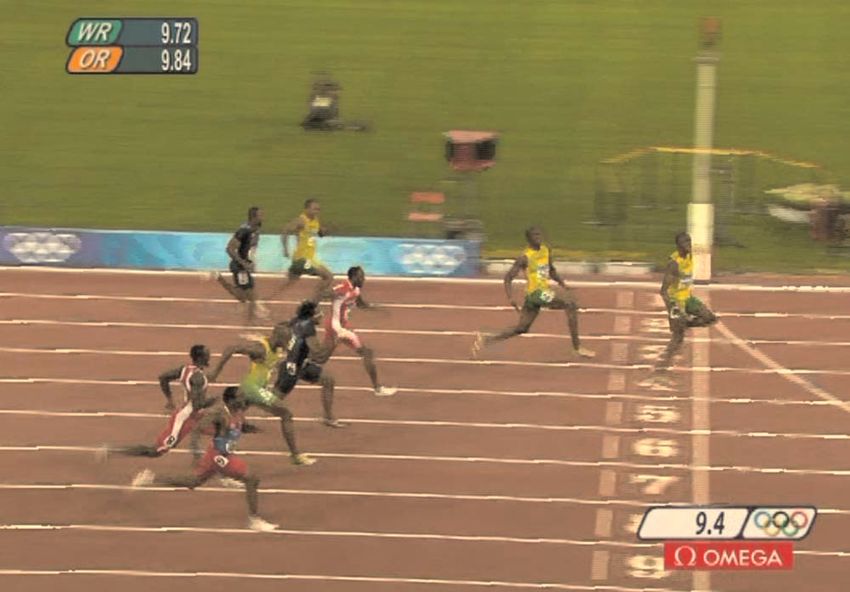
P

                                                                                                                                Bolt
                                                                                                            Thompson

                                                                            camera rail
Fig. 1. Example screen shot used to estimate the runners’ position as a
function of time.
                                                                              85
                                                                                    86
                                                                                          87
function of time, from which the first and second derivatives                                  88
                                                                                                     89
共i.e., speeds and accelerations兲 may be derived.                                                            90
   To make the projections we consider two scenarios. We                                                           91
first conservatively assume that Bolt would have been able to                                                              92
keep up with Thompson’s acceleration profile in the race                                                                               93
after 8 s of elapsed time and project a new finishing time.
Given his clearly higher acceleration around 6 s, we also                 Fig. 2. Schematic illustration of the main procedure for estimating the run-
consider a scenario in which he is able to maintain a                     ners’ positions: Two known parallel lines, orthogonal to the track, are ex-
                                                                          tended to find the horizon crossing point P for each frame. Auxilliary lines
⌬a = 0.5 m / s2 greater acceleration than Thompson to the fin-            are drawn from P onto the track, corresponding to each of the runners’
ish.                                                                      current positions. The positions are read off from the rail. This method was
   The new projected world record is found by extrapolating               used in the second half of the race. In the first half, in which there were
the resulting motion profile to 100 m. We estimate the uncer-             strong camera perspective effects, other methods were also used. See the
tainty in this number by repeating the analysis 10 000 times,             text for details.
each time adding a random fluctuation with specified uncer-
tainties to each time and tick count.
                                                                          synchronized, while in the rest the screen clock lags behind
III. DATA AND CALIBRATION                                                 by 0.1 s. We assume that the stadium clock is the correct
                                                                          one, and recalibrate the screen clock by adding an additional
   The data used for this analysis consist of three clips filmed          0.04 s to each time measurement. With these assumptions it
by three cameras located along the finishing line at slightly             is straightforward to calibrate both the clock and distance
different positions. Unfortunately, the NRK and BBC clips                 measurements, as is shown in the corresponding columns in
were filmed with cameras positioned fairly close to the track,            Table I.
and the rail of the moving camera therefore disappears out-
side the field of view after about 6 s. This problem does not             IV. ESTIMATION OF MOTION PROFILES
occur for the NBC clip, which was filmed from further away.
Using these data sets, we measured the position of Usain                     It is straightforward to make the desired projections using
Bolt and Richard Thompson at 16 different times in units of               the calibrated distance information. First, we compute a
ticks 共see Table I兲.                                                      smooth spline, s共t兲, through each of the two runners’ mea-
   There are three issues that must be addressed before the               sured positions. A bonus of using splines is that we automati-
tick counts listed in Table I can be converted into proper                cally obtain the first and second derivatives of s at each time
distance measurements. First, the camera rail is not entirely             step. To obtain a well-behaved spline we impose several
visible near the starting line, because the very first part is            constraints. We add two auxiliary data points at t = 0.01 s and
obscured by a cameraman. The tick counts in Table I are                   t = 13.0 s. These points are included to guarantee sensible
therefore counted relative to the first visible tick. Fortunately,        boundary conditions at each end. The first point implies that
it is not very problematic to extrapolate into the obscured               the starting velocity is zero, and the last one leads to a
region by using the distance between the visible ticks, and               smooth acceleration at the finishing line. We also adopt a
knowing that the distance between the starting line for the               smooth spline stiffness parameter of ␣ = 0.5 to minimize un-
100 m dash and 110 m hurdles is precisely 10 m. We esti-                  physical fluctuations.4 The results are fairly insensitive to the
mate the number of obscured ticks to be 7 ⫾ 1.                            value of ␣.
   Second, the precision of the screen clock is only a tenth of              The resulting functions are plotted in Fig. 3. Notice that
a second, and the clock appears to truncate the time, rather              Bolt and Thompson are almost neck by neck up to 4 s, cor-
than to round it off. We therefore add 0.05 s to each time                responding to a distance of 35 m. Bolt’s gold medal is essen-
measurement, and assume that our time uncertainty to be                   tially won between 4 and 8 s. At 8 s Bolt decelerates notice-
uniform between −0.05 and 0.05 s.                                         ably, and Thompson equalizes and surpasses Bolt’s speed.
   Finally, the screen clock on the clips is not calibrated per-          However, Thompson is not able to maintain his speed to the
fectly with the stadium clock 共see Fig. 1 for an example                  finish, but slows down after about 8.5 s. Still, his accelera-
frame兲. A little more than half of all frames appear to be                tion is consistently higher than Bolt’s after 8 s.

225         Am. J. Phys., Vol. 77, No. 3, March 2009                                                                       Eriksen et al.         225
Table I. Compilation of distance 共m兲 versus time 共s兲 for Usain Bolt and Richard Thompson in the 100 m dash
at Beijing 2008. The data for the second and last rows are not real observations, but ensure sensible boundary
conditions for the smooth spline. The second row ensures zero starting velocity, and the last row gives a smooth
acceleration at the finishing line. The data for t = 0.0 are taken from the known starting position and therefore
have zero uncertainty, and the data for t = 9.69 and t = 9.89 are taken from a high-resolution picture of the finish.
These times are not read from the screen clock, but are adopted from official sources. Zero uncertainties are
assigned to these points.
Bolt Thompson
Elapsed time Ticks Distance Ticks Distance Uncertainty Data set
0.0 −7.0 0.0 −7.0 0.0 0.0 None
0.01 −7.0 0.0 −7.0 0.0 0.0 None
1.1 −2.0 5.0 −2.1 4.9 0.5 NRK
3.0 15.5 22.5 15.6 22.6 0.5 NRK
4.0 27.0 34.0 27.0 34.0 0.4 NRK
4.5 34.3 41.3 34.1 41.1 0.5 NRK
5.4 45.1 52.1 44.3 51.3 0.5 NBC
5.8 48.9 55.9 48.3 55.3 0.5 BBC
6.2 54.5 61.5 53.8 60.8 0.5 NBC
6.5 57.8 64.8 56.9 63.9 0.4 BBC
6.9 62.6 69.6 61.5 68.5 0.2 NBC
7.3 66.3 73.3 65.1 72.1 0.2 NBC
7.7 71.5 78.5 70.1 77.1 0.2 NBC
8.0 74.7 81.7 72.9 79.9 0.2 NBC
8.3 78.6 85.6 76.8 83.8 0.2 NBC
8.6 82.2 89.2 80.5 87.5 0.2 NBC
8.8 84.3 91.3 82.4 89.4 0.2 NBC
9.4 91.6 98.6 89.4 96.4 0.2 NBC
9.69 93.0 100.0 ¯ ¯ 0.0 None
9.89 ¯ ¯ 93.0 100.0 0.0 None
13 105 112 105 112 5.0 None
100
It is important to note that there are significant uncertain- Usain Bolt
Distance (m)
80 Richard Thompson
ties related to these measurements, as indicated by the 68%
confidence regions 共gray bands兲 in Fig. 3. The acceleration 60
profile is particularly noisy 共that is, it exhibits unphysical
40
fluctuations兲, because it is estimated by numerically differen-
tiating the observed distance versus time data twice. 20
Another point is the fact that the velocity and acceleration
20
profiles for Bolt and Thompson correspond very closely with
each other. The reason is that the two main uncertainties in
Speed (m/s)
15
determining the position and time for each runner in a given
frame are common. We have to define a proper reference line
10
normal to the track in each frame, and the screen clock has a
temporal resolution of 0.1 s. These two effects result in large
5
and common uncertainties. These errors are modeled by a
Monte Carlo simulation, and the resulting uncertainties are
therefore properly propagated to the final results. 10
Acceleration (m/s )
2
5
V. WORLD RECORD PROJECTIONS
We can now answer the original question: How fast would 0
Bolt have run if he had not celebrated the last 2 s? To make
this projection we consider two scenarios: -5
共1兲 Bolt matches Thompson’s acceleration profile after 8 s. -10
共2兲 Bolt maintains a 0.5 m / s2 higher acceleration than 0 2 4 6 8
Thompson after 8 s. Elapsed time (s)
Fig. 3. Estimated position 共top兲, speed 共middle兲, and acceleration 共bottom兲
The justification of the first scenario is obvious, as Bolt out- for Bolt 共solid curves兲 and Thompson 共dashed-dotted curves兲 as a function
ran Thompson between 4 and 8 s. The justification of the of time. Actual distance measurements are indicated in the top panel with 5
second scenario is more speculative, because it is difficult to error bars. Gray bands indicate the 68% confidence regions for the spline
quantify exactly how much stronger Bolt was. If we look at estimators as estimated by Monte Carlo simulations.
226 Am. J. Phys., Vol. 77, No. 3, March 2009 Eriksen et al. 226Celebration begins World record
100
Distance (m)
90
80
70
7.6 7.8 8 8.2 8.4 8.6 8.8 9 9.2 9.4 9.6 9.8 10
(a) Elapsed time (s)
Fig. 5. Photo montage showing Bolt’s position relative to his competitors
Potential world records Actual world record
for the real 共left Bolt兲 and projected 共right Bolt兲 world records.
100
actual trajectory, s共t兲. For comparison, Thompson’s trajec-
tory is also indicated.
Distance (m)
The projected new world record is the time at which ŝ共t兲
equals 100 m. We include 95% statistical errors estimated by
98
Monte Carlo simulations as described in Sec. II and find that
the new world record would be 9.61⫾ 0.04 s in the first sce-
nario and 9.55⫾ 0.04 s in the second scenario.
Usain Bolt (optimistic projection)
Usain Bolt (conservative projection)
96
Richard Thompson (measured)
VI. CONCLUSIONS
Usain Bolt (measured)
Glen Mills, Usain Bolt’s coach, suggested that the world
9.4 9.45 9.5 9.55 9.6 9.65 9.7 9.75 9.8 9.85 record could have been 9.52 s if Bolt had not danced along
(b) Elapsed time (s) the track in Beijing for the last 20 m. According to our cal-
culations, this suggestion seems like a good, but probably an
Fig. 4. 共a兲 Comparison of real and projected distance profiles at the end of optimistic, estimate. Depending on assumptions about Bolt’s
the race. The point where the profiles cross the horizontal 100 m line is the
new world record for a given scenario; 共b兲 is a zoomed version of 共a兲. The
acceleration at the end of the race, we find that his time
dashed line shows the first scenario, and the dotted line shows the second would have been somewhere between 9.55 and 9.61 s, with a
scenario; the actual trajectory, s共t兲 is shown as a solid line. For comparison, 95% statistical error of ⫾0.04 s. The uncertainties due to the
Thompson’s trajectory is indicated by a dashed-dotted line. assumptions about the acceleration are comparable to or
larger than the statistical uncertainties. Therefore, 9.52 s is
not out of reach.
the acceleration profiles in Fig. 3 and note that Bolt is con- In Fig. 5 we show an illustration of how such a record
sidered a 200 m specialist, a value of 0.5 m / s2 seems realis- would compare to the actual world record of 9.69 s, relative
tic. 共Negative accelerations are always observed in 100 m to the rest of the field: The left version of Bolt shows his
races; nobody is able to maintain their full speed to the fin- actual position at ⬃9.5 s, while the right version indicates
ishing line.5 Assuming for instance constant speed during the his position in the new scenarios.
last 2 s would therefore predict an unrealistically good time.兲 There are several potential systematic errors involved in
For each scenario we computed a trajectory for Bolt by these calculations. For instance, it is impossible to know for
choosing the initial conditions s0 = s共8 s兲 and v0 = v共8 s兲 and sure whether Usain Bolt might have tired at the end, which
an acceleration profile as described. The computation of would increase the world record beyond our estimates. Judg-
these trajectories are performed by integrating the kinematic ing from his facial expressions as he crossed the finishing
line, this hypothesis does not strike us as very plausible.
再 冎
equations with respect to time,
Another issue to consider is the wind. It is generally
aThompson共t兲 共Scenario 1兲 agreed that a tail wind speed of 1 m / s improves a 100 m
â共t兲 = 共1兲
aThompson共t兲 + 0.5 m/s 共Scenario 2兲, time by 0.05 s.6,7 For the International Association of Athlet-
ics Federations to acknowledge a run as a record attempt, the
v̂共t兲 = v0 + 冕 t0
t
â共t兲dt, 共2兲
wind speed must be less than +2 m / s. When Bolt ran in
Beijing, there was no measurable wind speed, and we can
therefore safely assume that the world record could have
冕 t
been further decreased, perhaps by as much as 0.1 s, under
more favorable wind conditions.
ŝ共t兲 = s0 + v̂共t兲dt. 共3兲
t0
It is interesting to note that Usain Bolt had the slowest
start reaction time of the field, 0.025 s slower than Richard
In Fig. 4 we compare the projected trajectories, ŝ共t兲, with the Thompson according to official measurements found on
227 Am. J. Phys., Vol. 77, No. 3, March 2009 Eriksen et al. 227a兲
IAAF’s webpage. All of these issues considered together Electronic mail: h.k.k.eriksen@astro.uio.no
b兲
suggests that a new world record of less than 9.5 s is within Electronic mail: j.r.kristiansen@astro.uio.no
c兲
Electronic mail: oystein.langangen@astro.uio.no
reach by Usain Bolt in the near future. d兲
Electronic mail: i.k.wehus@fys.uio.no
1
J. B. Keller, “A theory of competitive running,” Phys. Today 26共9兲,
43–47 共1973兲.
ACKNOWLEDGMENTS 2
R. Tibshirani, “Who is the fastest man in the world?,” Am. Stat. 51共2兲,
106–111 共1997兲.
First and foremost, the authors would like to thank Chris- 3
J. R. Mureika, “A realistic quasi-physical model of the 100 m dash,” Can.
tian Nitschke Smith at NRK Sporten for providing very use- J. Phys. 79共4兲, 697–713 共2001兲.
4
ful high-resolution footage of the Beijing 100 m run, and P. J. Green, and B. W. Silverman, Non-Parametric Regression and Gen-
BBC and NBC for making their videos available on their eralized Linear Models 共Chapman and Hall, London, 1994兲.
5
F. Mathis, “The effect of fatigue on running strategies,” SIAM Rev.
web pages. The authors would also like to thank John D. 31共2兲, 306–309 共1989兲.
Barrow and Dmitris Evangelinos for useful feedback, and 6
J. D. Barrow, “Frank’s fastest,” Athletics Weekly, 6 August, 1997.
Steve Alessandrini for reproducing the authors’ spline fits 7
J. R. Mureika, “The legality of wind and altitude assisted performances in
and providing them with his MATLAB code. the sprints,” New Studies Athletics 15共3/4兲, 53–60 共2000兲.
228 Am. J. Phys., Vol. 77, No. 3, March 2009 Eriksen et al. 228You can also read