CBP: Backpropagation with constraint on weight precision using pseudo-Lagrange multiplier method
←
→
Page content transcription
If your browser does not render page correctly, please read the page content below
CBP: Backpropagation with constraint on weight
                                             precision using pseudo-Lagrange multiplier method

                                                                             Guhyun Kim, Doo Seok Jeong∗
                                                                      Division of Materials Science and Engineering
                                                                         Hanyang University, Republic of Korea
arXiv:2110.02550v2 [cs.LG] 25 Oct 2021

                                                                 guhyunkim01@gmail.com, dooseokj@hanyang.ac.kr

                                                                                         Abstract

                                                     Backward propagation of errors (backpropagation) is a method to minimize objec-
                                                     tive functions (e.g., loss functions) of deep neural networks by identifying optimal
                                                     sets of weights and biases. Imposing constraints on weight precision is often
                                                     required to alleviate prohibitive workloads on hardware. Despite the remarkable
                                                     success of backpropagation, the algorithm itself is not capable of considering such
                                                     constraints unless additional algorithms are applied simultaneously. To address
                                                     this issue, we propose the constrained backpropagation (CBP) algorithm based on
                                                     the pseudo-Lagrange multiplier method to obtain the optimal set of weights that
                                                     satisfy a given set of constraints. The defining characteristic of the proposed CBP
                                                     algorithm is the utilization of a Lagrangian function (loss function plus constraint
                                                     function) as its objective function. We considered various types of constraints
                                                     — binary, ternary, one-bit shift, and two-bit shift weight constraints. As a post-
                                                     training method, CBP applied to AlexNet, ResNet-18, ResNet-50, and GoogLeNet
                                                     on ImageNet, which were pre-trained using the conventional backpropagation. For
                                                     most cases, the proposed algorithm outperforms the state-of-the-art methods on
                                                     ImageNet, e.g., 66.6%, 74.4%, and 64.0% top-1 accuracy for ResNet-18, ResNet-
                                                     50, and GoogLeNet with binary weights, respectively. This highlights CBP as a
                                                     learning algorithm to address diverse constraints with the minimal performance
                                                     loss by employing appropriate constraint functions. The code for CBP is publicly
                                                     available at https://github.com/dooseokjeong/CBP.

                                         1       Introduction
                                         Currently, deep learning-based methods are applied in a variety of tasks, including the classification
                                         of static data, e.g., image recognition [1, 2]; classification of dynamic data, e.g., speech recogni-
                                         tion [3–6]; function approximations, which require the output of precise predictions, e.g., electronic
                                         structure predictions [7] and nonlinear circuit predictions [8]. All of the aforementioned tasks require
                                         discriminative models. Additionally, generative models, including generative adversarial networks [9]
                                         and variants [10–13], comprise another type of deep neural network. Despite the diversity in applica-
                                         tion domain and model type used, almost all deep learning-based methods use backpropagation as a
                                         common learning algorithm.
                                         Recent developments in deep learning have primarily focused on increasing the size and depth
                                         of deep neural networks (DNNs) to improve their learning capabilities as in the case of state-of-
                                         the-art DNNs like VGGNet [14] and ResNet [15]. Given that the memory capacity required by a
                                         DNN is proportional to the number of parameters (weights and biases), memory usage for DNN
                                         becomes severe. Additionally, a significant number of multiply-accumulate operations during the
                                             ∗
                                                 Corresponding author

                                         35th Conference on Neural Information Processing Systems (NeurIPS 2021), Sydney, Australia.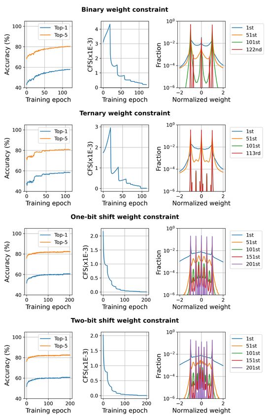
training and inference stages impose prohibitive workload on hardware. Thus, efficient hardware-
resource consumption is critical to the optimal performance of deep learning. One way to address
this requirement is the use of weights of limited precision, such as binary [16, 17] and ternary
weights [18, 19]. To this end, particular constraints are applied to weights during training, and
additional algorithms for weight quantization are used in conjunction with backpropagation. This is
because such constraints are not considered during the minimization of the objective function (loss
function) when backpropagation is executed.
We adopt the Lagrange multiplier method (LMM) to combine basic backpropagation with additional
constraint algorithms and produce a single constrained backpropagation (CBP) algorithm. We refer
to the adopted method as pseudo-LMM because the constraint functions cs (x) are nondifferentiable
at xm (= arg minx cs (x)), rendering LMM inapplicable. Nevertheless, pseudo-LMM successfully
attains the optimal point under particular conditions as for LMM. In the CBP algorithm, the optimal
weights satisfying a given set of constraints are evaluated via a basic backpropagation algorithm.
It is implemented by simply replacing the conventional objective function (loss function) with
a Lagrangian function L that comprises the loss and constraint functions as sub-functions that
are subjected to simultaneous minimization. Therefore, this method is perfectly compatible with
conventional deep learning frameworks. The primary contributions of this study are as follows.

       • We introduce a novel and simple method to incorporate given constraints into backpropa-
         gation by using a Lagrangian function as the objective function. The proposed method is
         able to address any set of constraints on the weights insomuch as the constraint functions
         are mathematically well-defined.
       • We introduce pseudo-LMM with constraint functions cs (w) that are nondifferentiable at
         wm (= arg minw cs (w)) and analyze the kinetics of pseudo-LMM in the continuous time
         domain.
       • We introduce optimal (sawtooth-like) constraint functions with gradually vanishing
         unconstrained-weight windows and provide a guiding principle for the stable co-optimization
         of weights and Lagrange multipliers in a quasi-static fashion.
       • We evaluate the performance of CBP applied to AlexNet, ResNet-18, ResNet-50, and
         GoogLeNet (pre-trained using backpropagation with full-precision weights) with four
         different constraints (binary, ternary, one-bit shift, and two-bit shift weight constraints) on
         ImageNet as proof-of-concept examples. The results highlight the classification accuracy
         outperforming the previous state-of-the-art results.

2   Related work
The simplest approach to weight quantization is the quantization of pre-trained weights. Gong et
al. [20] proposed several methods for weight quantization and demonstrated that binarizing weights
using a sign function degraded the top-1 accuracy on ImageNet by less than 10%. Mellempudi et
al. [21] proposed a fine-grained quantization algorithm that calculates the optimal thresholds for the
ternarization of pre-trained weights. The expectation backpropagation algorithm [22] implements a
variational Bayesian approach to weight quantization. It uses binary weights and activations during
the inference stage. Zhou et al. [23] proposed the incremental network quantization method (INQ)
that iteratively re-trains a group of weights to compensate for the performance loss caused by the rest
of weights which are quantized using pre-set quantization thresholds.
Several methods of weight quantization utilize auxiliary real-valued weights in conjunction with
quantized weights during training. The straight-through-estimator (STE) comprises the conduction of
forward and backpropagation using quantized weights but relies on the auxiliary real-valued weights
for the update of weights [3]. BinaryConnect [16] utilizes weights binarized by a sign function for
forward and backpropagation, and the real-valued weights are updated via backpropagation with
binary weights. The binary-weight-network (BWN) [17] identifies the binary weights closest to
the real-valued weights using a scaling factor, and it exhibits a higher classification accuracy than
BinaryConnect on ImageNet. The binarized neural nets [24] and XNOR-Nets [17] are extensions of
BinaryConnect and BWN, respectively, which utilize binary activations alongside binary weights.
Lin et al. [18] proposed TernaryConnect and Ternary-weight-network (TWN), which are similar to
BinaryConnect and BWN but use weight-ternarization methods instead. Trained ternary quantization

                                                   2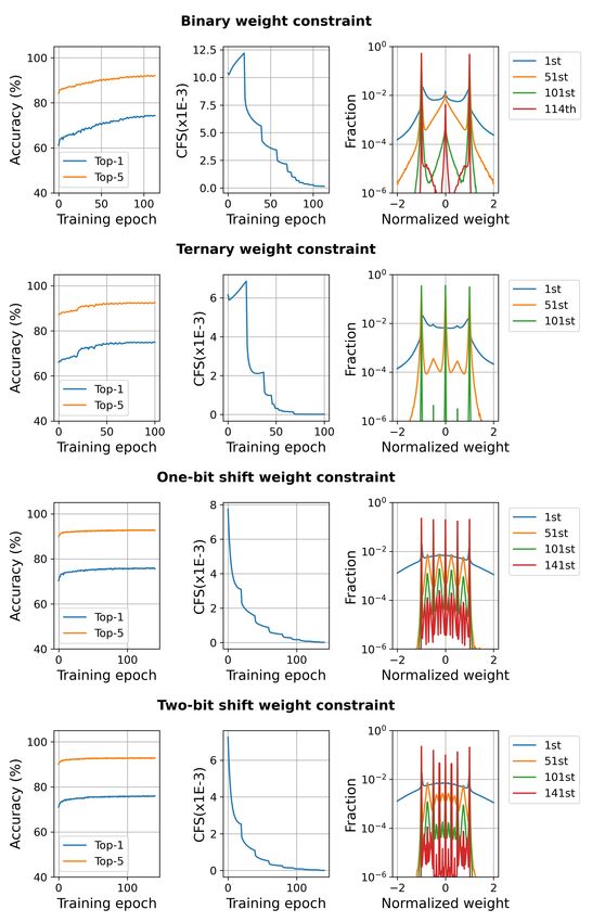
(TTQ) [25] also uses ternary weights that are quantized using trainable thresholds for quantization.
LQ-Nets proposed by Zhang et al. [26] utilize activation- and weight-quantizers considering the
actual distributions of full-precision activation and weight, respectively. DeepShift Network [27]
includes the LinearShift and ConvShift operators that replace the multiplications of fully-connected
layers and convolution layers, respectively. Qin et al. [28] introduced IR-Nets that feature the use
of error decay estimators to approximate sign functions for weight and activation binarization to
differentiable forms. Gong et al. [29] and Yang et al. [30] employed functions similar to step functions
but differentiable. Pouransari et al. [31] proposed the least squares quantization method that searches
proper scale factors for binary quantization. Elthakeb et al. [32] attempted to quantize weights and
activations by applying sinusoidal regularization. The regularization involves two hyperparameters
that determine weight-quantization and bitwidth-regularization strengths.
To take into account the constraint on weight precision, Leng et al. [33] used an augmented Lagrangian
function as an objective function, which includes a constraint-agreement sub-function. The method
was successfully applied to various DNNs on ImageNet; yet, the method failed to reach the accuracy
level for full-precision models even when 3-bit precision was used.
The CBP algorithm proposed in this study also utilizes LMM; but CBP essentially differs from
[33] given that (i) the basic differential multiplier method (BDMM), rather than ADMM, is used to
apply various constraints on weight precision, (ii) particularly designed constraint functions with
gradually vanishing unconstrained-weight windows are used, and (iii) substantial improvement on
the classification accuracy on ImageNet is achieved.

3     Optimization method
3.1   Pseudo-Lagrange multiplier method

LMM calculates the maximum or minimum value of a differentiable function f under a differentiable
constraint cs = 0. [34] Let us assume that a function f (x, y) attains its minimum (or maximum)
value m satisfying a given constraint at (xm , ym ), i.e., f (xm , ym ) = m. Further, cs (xm , ym ) = 0
as the constraint is satisfied at this point. In this case, the point of intersection between the graphs of
the two functions, f (x, y) = m and cs (x, y) = 0, is (xm , ym ). Because the two functions have a
common tangent at the point of intersection, the following equation holds:
                                          ∇x,y f = −λ∇x,y cs,                                          (1)
at (xm , ym ), where λ is a Lagrange multiplier [35].
The Lagrangian function is defined as L (x, y, λ) = f (x, y) + λcs (x, y). Consider a lo-
cal point (x, y) at which the gradient of L (x, y, λ) is zero. Therefore, ∇x,y,λ L (x, y, λ) =
∇x,y [f (x, y) + λcs (x, y)] + ∇λ [λcs (x, y)]. Thus, ∇x,y,λ L (x, y, λ) = 0 is equivalent to the
following equations.

                                                ∇x,y [f (x, y) + λcs (x, y)] = 0,
               ∇x,y,λ L (x, y, λ) = 0 ⇔
                                                             ∇λ [λcs (x, y)] = 0

                                                ∇x,y f (x, y) = −λ∇x,y cs (x, y)
                                       ⇔                                                      (2)
                                                   cs (x, y) = 0

This satisfies the condition in Eq. (1) as well as the constraint cs (x, y) = 0. Therefore, the local
point (x, y) corresponds to the minimum (or maximum) point of the function f under the constraint.
We define pseudo-LMM to address similar minimization tasks but with continuous constraint func-
tions that are nondifferentiable at (xm , ym ) = arg minx,y cs (x, y). Thus, Eq. (1) cannot be satisfied
at the optimal point. Nevertheless, pseudo-LMM enables us to minimize the function f (x) subject to
the constraint condition cs (x) = 0 using the Lagrangian function L (x, λ).
Definition 3.1 (Pseudo-LMM). Pseudo-LMM is a method to attain the optimal variables xm that
minimize function f (x) subject to the constraint condition cs (x) = 0, where the function cs (x) is
nondifferentiable at xm but reaches the minimum at xm , i.e., cs (xm ) = 0.
Theorem 3.1. Minimizing the Lagrangian function L (x, λ), which is given by L (x, λ) = f (x) +
λcs (x), is equivalent to minimizing the function f (x) subject to cs (x) = 0

                                                    3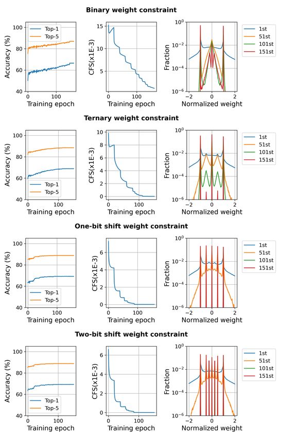
Proof. The Lagrangian function L (x, λ) is always differentiable with respect to the Lagrangian
multiplier λ, so that the equation cs (x) = 0 holds at the optimal point xm . Thus, we have
                                                (
                                                  minimize L(x; λ)
                           minimize L (x, λ) ⇔         x                                    (3)
                              x,λ                 subject to cs (x) = 0.

When the constraint is satisfied, i.e., cs (x) = 0, the Lagrangian function L (x; λ) equals the function
f (x), so that the task to minimize L (x, λ) with respect to x and λ corresponds to the task to
minimize f (x) subject to cs (x) = 0.

Given Theorem 3.1, pseudo-LMM can attain the optimal point by minimizing the Lagrangian function
L in spite of the nondifferentiability of the constraint function cs (x) = 0 at the optimal point xm .
Note that not all functions have zero gradients at their minimum points; for instance, the function
y = |x| attains its minimum at x = 0 but the gradient at the minimum point is not defined. However,
all convex functions have zero gradients at their minimum points. Thus, LMM to minimize the
function f (x) subject to the constraint convex function cs (x) with minimum point xm is a subset
of pseudo-LMM. In this case, the constraint function has zero gradient at the minimum point, so that
Eq. (2) becomes

                                                             ∇x f (x) = 0
                        ∇x,λ L (x, λ) = 0 ⇔                                                        (4)
                                                      subject to cs (x) = 0.

We will consider continuous constraint functions with a few nondifferentiable points in their variable
domains, including their minimum points. Other than such nondifferentiable points, we will use the
gradient descent method to search for the minimum points within the framework of pseudo-LMM.
Hereafter, when the gradient of the Lagrangian L function is remarked, its variable domain excludes
such nondifferentiable points.
The optimal solution to Eq. (4) can be found using the basic differential multiplier method
(BDMM) [36] that calculates the point at which L (x, λ) attains its minimum value by driving
x toward the constraint subspace x̄ (cs (x̄) = 0). The BDMM updates x and λ according to the
following relations.
                                    x ← x − ηx ∇x L (x, λ) ,                             (5)
and
                                      λ ← λ + ηλ ∇λ L (x, λ) .                                      (6)
BDMM is cheaper than Newton’s method in terms of computational cost. Additionally, Eq. (5) is
identical to the solution used in the gradient descent method during backpropagation, except for
the use of a Lagrangian function instead of a loss function. This indicates the compatibility of
pseudo-LMM with the optimization framework based on backpropagation.

3.2   Constrained backpropagation using the pseudo-Lagrange multiplier method

We utilize pseudo-LMM to train DNNs with particular sets of weight-constraints. We define a
Lagrangian function L in the context of feedforward DNN using the following relation.

                 L y (k) , ŷ (k) ; W , λ   = C y (k) , ŷ (k) ; W + λT cs (W ) ,       (7)
                                                                                T
                                      cs =      [cs1 (w1 ) , . . . , csnw (wnw )]
                                                                 T
                                       λ    =   [λ1 , . . . , λnw ] .

where y (k) and ŷ (k) denote the actual output vector for the kth input data and correct label, respec-
tively. The set W denotes a set of weight matrices, including nw weights in aggregate, and the
function C denotes a loss function. Each weight wi (1 ≤ i ≤ nw ) is given one constraint function
csi (wi ) and one multiplier λi .
We chose sawtooth-shaped constraint functions. We quantize the real-valued weights into nq values in
                 nq
the set Q = {qi }i=1 , where qi < qi+1 for all i. We also employ a set of the medians of neighboring

                                                   4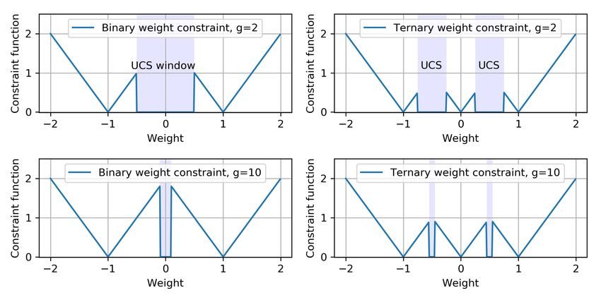
Figure 1: Binary- and ternary-weight constraint functions for g = 2 and 10. Blue-filled regions
indicate unconstrained-weight windows.

                                     n −1
                                     q
values in the set Q: M = {mi }i=1       , where mi = (qi + qi+1 ) /2. Using Q and M , we define a
partial constraint function yi for i = 0, 1 ≤ i < nq , and i = nq ,

                                    −2 (w − q1 ) if w < q1 ,
                  y0 (w) =
                                          0           otherwise,

                                    −2 |w − mi | + qi+1 − qi if qi ≤ w < qi+1 ,
                   yi (w) =
                                                0                otherwise,

                                    2 w − q nq    if w ≥ qnq ,
                 ynq (w) =                                                                    (8)
                                          0           otherwise,
respectively.
Pnq           The constraint function cs is the summation of the partial constraint functions Y (w) =
   i=0 yi (w), gated by the unconstrained-weight window ucs (w) parameterized by a variable g.
                                   cs (w; Q, M , g) = ucs (w) Y (w) ,                                      (9)
where
                                       nq −1
                                        X               1
                      ucs (w) = 1 −            H          (qi+1 − qi ) − |w − mi + | ,                   (10)
                                        i=0
                                                       2g
where  → 0+ , and H denotes the Heaviside step function. The function ucs (w) realizes the
unconstrained-weight window as a function of g (≥ 1). When g = 1, the function outputs zero for
q1 ≤ w < qnq , merely confining w to the range q1 ≤ w < qnq without weight quantization, whereas,
when g → ∞, the window vanishes, allowing the constraint function to quantize the weight in the
entire weight range. Examples of function ucs (w) are shown in Fig. 1.
The unconstrained-weight window variable g is initially set to one and updated such that it keeps
increasing during training, i.e., the window gradually vanishes. The window gradually vanishing
allows sequential weight quantization such that the further the initial weights from their nearest qi ,
the later their weights are subject to quantization, which is otherwise subject to simultaneous (abrupt)
quantization. It is likely that the further the initial weights from their nearest qi , the larger the increase
in loss function C when they are quantized. Thus, the sequential quantization from the weights close
to their qi likely avoids an abrupt increase in the loss. Further, while the closer weights are being
quantized, the further weights (not subject to quantization yet) are being updated to reduce the loss
given the partially quantized weights. This effect will be discussed in Sections 3.3 and 5.
For every training batch, the weights are updated following a method similar to conventional back-
propagation. Nevertheless, the use of the Lagrangian function in Eq. (8), rather than a loss function

                                                          5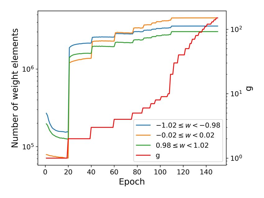
only, as an objective function constitutes a critical difference. The Lagrange multipliers λ are sub-
sequently updated using the gradient ascent method in Eq. (6). Updating cross-coupled variables,
such as W and λ, often experiences difficulties in convergence toward the optimal values because of
oscillation around the optimal values. A feasible solution involves quasi-static update. To this end,
we significantly reduce the update frequency of the Lagrange multipliers λ compared with weights
W.
Weight update: Weights W are updated once every iteration as for the conventional backpropagation
but using the Lagrangian function L.
Lagrange multiplier update: Lagrange multipliers λ are conditionally updated once every training
epoch. The update is allowed if the summation of all L in a given epoch (Lsum ) is not smaller than
Lsum for the previous epoch (Lpresum ) or the multipliers λ have not been updated in the past pmax
epochs. This achieves the convergence of W for a given λ in a quasi-static manner.
Unconstrained weight window update: Unconstrained-weight window variable g is updated on
the same condition as for the Lagrange multipliers λ. Unlike weights W and multipliers λ, the
variable g (initialized to one) constantly increases when updated such that ∆g = 1 when g < 10,
∆g = 10 for 10 ≤ g < 100, and ∆g = 100 otherwise.
The detailed learning algorithm is shown in the pseudocode in Appendix A.2.

3.3   Learning kinetics

Learning with BDMM using the Lagrangian function is better understood in the continuous time
domain. We first address the kinetics of learning without the unconstrained-weight window ucs (w).
The change in the Lagrangian function L at a given learning step in the discrete time domain is
equivalent to the derivative of L with time at time t in the continuous time domain, which is given by
                                       nw                    2         nw
                         dL        −1
                                       X     ∂C         ∂csi            X
                             = −τW                 + λi          + τλ−1     cs2i .                 (11)
                          dt           i=0
                                             ∂w  i       ∂w i           i=0

The Lagrange multiplier λi at time t is given by
                                                              Z   t
                                     λi (t) = λi (0) + τλ−1           csi dt.                        (12)
                                                              0

Eqs. (11) and (12) are derived in Appendix A.1. The constraint functions csi approach zero as the
weights approach their corresponding quantized values qi , and thus the Lagrange multipliers in Eq.
(12) asymptotically converge to their limits.
At equilibrium, the Lagrange function is no longer time-dependent, i.e., dL/dt = 0. This requires
the Lagrange multipliers reaching their limits, which in turn requires the weights reaching their
corresponding quantized values W ∗cs , leading to cs = 0. For convenience, we define the integration
of csi in Eq. (12) as ∆csi (≥ 0).
                                    Z t
                             ∆csi =      csi dt, if csi → 0 as t → ∞.                           (13)
                                          0

Thus, the equilibrium Lagrange multiplier λ∗cs
                                           i   can be expressed as
                                        λ∗cs
                                         i   = λi (0) + τλ−1 ∆csi .                                  (14)
Therefore, it is evident from Eq. (11) that the equilibrium leads to
                                     ∂C                          ∂csi
                               ∀i,       = − λi (0) + τλ−1 ∆csi        .                             (15)
                                     ∂wi                          ∂wi
We consider sawtooth constraint functions with slopes ±s, i.e., ∂csi /∂wi = ±s, where s > 0.
Eq. (8) is the case of s = 2. Generally, the Lagrange multiplier is initialized to zero, i.e., λi (0) = 0.
Therefore, the gradient of loss function C at the equilibrium point W ∗cs is given by
                                        ∂C
                                  ∀i,       = ±τλ−1 s∆csi = ±λ∗cs
                                                              i s.                                   (16)
                                        ∂wi

                                                    6
Consider that the loss function C has the equilibrium point W ∗ = arg minW C . Eq. (16) eluci-
dates the increase of loss by attaining the equilibrium point W ∗cs . In this regard, λ∗cs
i corresponds
to the cost of weight quantization. Assuming the convexity of the loss function C in a domain D
including W ∗ and W ∗cs , C (W ∗cs ) keeps increasing as λ∗cs i increases. If the initial pre-trained
weights equal their corresponding quantized weights, i.e., wi∗ = wi∗cs , then ∆csi = 0, and thus
λ∗cs
i = 0 according to Eq. (14). Eq. (16) consequently yields ∂C/∂wi = 0, indicating zero cost of
quantization.
Considering the gradually vanishing unconstrained-weight window ucs (w) yields the derivative of
L with time at time t in the continuous time domain as follows.
nw 2 nw
dL −1
X ∂C ∂Yi X 2
= −τW + λi ucsi + τλ−1 (ucsi Yi ) . (17)
dt i=0
∂w i ∂wi i=0
The derivation of Eq. (17) is given in Appendix A.3. Distinguishing the weights in the unconstrained-
weight window Ducs from the others at a given time t, Eq. (17) can be written by
" #
dL X ∂C 2 X
∂C ∂Yi
2
−1 −1 −1 2
= −τW − τW + λi − τλ Yi . (18)
dt ∂wi ∂wi ∂wi
wi ∈Ducs wi ∈D
/ ucs
The latter term on the right-hand side of Eq. (18) indicates that the weights outside the window Ducs
are being quantized at the cost of increase of loss. However, as indicated by the former term, the
weights in the window Ducs are being optimized only to decrease the loss function with partially
quantized weights. Compare this gradual quantization with abrupt quantization without the gradually
vanishing unconstrained-weight window, where all weights are subject to simultaneous (abrupt)
quantization. The gradual quantization allows the weights in the window to further reduce the loss
function regarding the weights that have already been quantized or are being quantized, and thus the
eventual cost of quantization is likely smaller than the simultaneous quantization case.
4 Experiments
To evaluate the performance of our algorithm, we trained three models (AlexNet, and ResNet-18
and 50) on the ImageNet dataset [37] with four different weight constraints (binary, ternary, and
one-bit, and two-bit shift weight constraints). ImageNet consists of approximately 1.2 million training
images and 50 thousands validation images. All training images were pre-processed such that they
were randomly cropped and resized to 224 × 224 with mean subtraction and variance division.
Additionally, random horizontal flipping and color jittering were applied. For validation, the images
were resized to 256 × 256 and their centers in 224 × 224 were cropped. We evaluated the top-1 and
top-5 classification accuracies on the validation set.
We considered binary, ternary, one-bit shift and two-bits shift weight constraints to validate the
CBP algorithm as a general weight-quantization framework. For all cases, we introduced layer-wise
scaling factors a such that a(l) (for the lth layer) is given by a(l) = kW (l) k1 /n(l) , where W (l) and
n(l) denote the weight matrix of the lth layer and the number of elements of W (l) , respectively. As
for [17] and [19], the weight matrices of the first and last layers were not quantized. The quantized
weights employed for each constraint case is elaborated as follows.
Binary-weight constraint: A set of quantized weights Q is {−a, a}.
D
The other weight constraints: A set of quantized weights Q is 0, ±2−d a d=0 , where D = 0, 1
and 2 for the ternary, one-bit shift, and two-bit shift weight constraints. Each ternary weight needs
2-bit memory while each of one-bit and two-bit shift weight needs 3-bit memory.
We adopted the STE [38] to train the models such that the forward pass is based on quantized weights
wq ,
nq −1
X
wq = q1 + (qi+1 − qi ) (sign (w − mi ) + 1) /2,
i=1
whereas the backward pass uses the real-valued weights w that are subject to quantization, ∂L/∂w =
∂L/∂wq .
7For all cases, the DNN was pre-trained using conventional backpropagation with full-precision
weights and activations, which was followed by post-learning using CBP. We used the stochastic
gradient descent with momentum to minimize the Lagrangian function L with respect to W and
Adam [39] to maximize L with respect to λ. The initial multiplier-learning rate ηλ and pmax were
set to 10−4 and 20, respectively. The weight-learning rate ηW decreased to 10−1 times the initial rate
when g reached 20 for all cases except GoogLeNet with the binary-weight constraint (the weight-
learning rate decayed when g = 200). The hyperparameters used are shown in Appendix A.5, which
were found using manual searches.
By asymptotically minimizing the Lagrangian function L, the constraint function cs (W ) approaches
0. The degree of constraint-failure per weight was evaluated based on the constraint-failure score
(CF S), which is defined as
nw
1 X
CF S = Yi (wi ; Q, M ) , (19)
nw i=1
where nw denotes the total number of weights. The CBP algorithm was implemented in Python on a
workstation (CPU: Intel Xeon Silver 4110 2.10GHz, GPU: Titan RTX).
It should be noted that we used CBP as a post-training method, so that the random seed effect is
involved only when organizing the mini-batches. The accuracy deviation is consequently marginal.
Table 1: Top-1/Top-5 accuracy of AlexNet, ResNet-18, ResNet-50, and GoogLeNet on ImageNet
Algorithm Binary Ternary One-bit shift Two-bit shift Full-precision
AlexNet
BWN [17] 56.8%/79.4% - - -
ADMM [33] 57.0%/79.7% 58.2%/80.6% 59.2%/81.8% 60.0%/82.2%
LQ-Nets [26] - 60.5%/82.7% - - 60.0%/82.4%
TTQ [25] - 57.5%/79.7% - -
CBP 58.0%/80.6% 58.8%/81.2% 60.8%/82.6% 60.9%/82.8%
ResNet-18
BWN [17] 60.8%/83.0% - - -
TWN [19] - 61.8%/84.2% - -
INQ [23] - 66.0%/87.1% - 68.1%/88.4%
ADMM [33] 64.8%/86.2% 67.0%/87.5% 67.5%/87.9% 68.1%/88.3%
69.6%/89.2%
QN [30] 66.5%/87.3% 69.1%/88.9% 69.9%/89.3% 70.4%/89.6%
IR-Nets [28] 66.5%/86.8% - - -
LQ-Nets [26] - 68.0%/88.0% - 69.3%/88.3%
TTQ [25] - 66.6%/87.2% - -
DSQ [29] 63.71%/- - - -
LS [31] 66.1%/86.5 - - -
CBP 66.6%/87.1% 69.1%/89.0% 69.6%/89.3% 69.6%/89.3%
ResNet-50
BWN [17] 63.9%/85.1% - - -
TWN [19] - 65.6%/86.5% - -
76.0%/93.0%
ADMM [33] 68.7%/88.6% 72.5%/90.7% 73.9%/91.5% 74.0%/91.6%
QN [30] 72.8%/91.3% 75.2%/92.6% 75.5%/92.8% 76.2%/93.2%
CBP 74.4%/92.1% 75.1%/92.5% 76.0%/92.9% 76.0%/92.9%
GoogLeNet
BWN [17] 59.0%/82.4% - - -
TWN [19] - 61.2%/86.5% - -
71.0%/90.8%
ADMM [33] 60.3%/83.2% 63.1%/85.4% 65.9%/87.3% 66.3%/87.5%
CBP 64.0%/86.0% 66.0%/87.3% 69.8%/89.7% 70.5%/90.1%
4.1 AlexNet
AlexNet is a simple convolutional networks which consists of five convolutional layers and three
fully-connected layers [2]. We used AlexNet with batch normalization [40] as in [17, 19, 33]. The
initial weight-learning rate ηW was set to 10−3 for the binary- and ternary-weight constraints and
810−4 for the other constraints. The batch size was set to 256. We used a weight decay rate (L2-
regularization) of 5 × 10⁻⁴ . The CBP algorithm exhibited state-of-the-art results as listed in Table. 1.
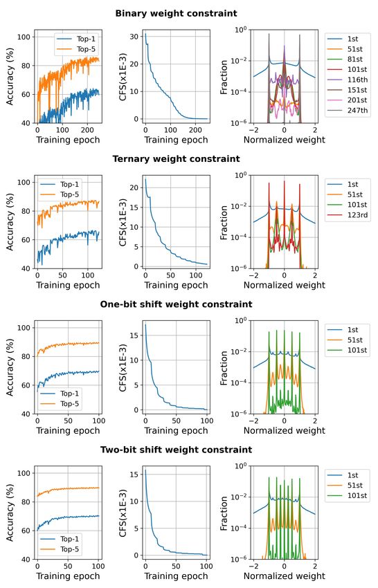
The detailed behaviors of networks with binary- and ternary-weight constraints are addressed in
Appendix B. The behaviors highlight asymptotic increases in the top-1 and top-5 recognition accuracy
with asymptotic decrease in CF S. Consequently, the weight distribution bifurcates asymptotically,
fulfilling the constraints imposed on the weights.
4.2 ResNet-18 and ResNet-50
We also evaluated our algorithm on ResNet-18 and ResNet-50 [15] which were pre-trained using
conventional backpropagation. For ResNet-18, the initial weight-learning rate ηW was set to 10−3
for all constraint cases. The batch size was 256. For ReNet-50, the initial weight-learning rate ηW
was set to 10−3 for binary- and ternary-weight constraints and 10−4 for the other cases. The batch
size was set to 128. The weight decay rate (L2-regularization) was set to 10−4 for both ResNet-18
and ResNet-50. The results are summarized in Table 1, highlighting state-of-the-art performance
compared with previous results. Notably, CBP with the one- and two-bit shift weight constraints
almost reaches the performance of the full-precision networks. Particularly, for ResNet-50, CBP
with the binary-weight constraint significantly outperforms other methods. The detailed behaviors of
weight quantizations for ResNet-18 and ResNet-50 are addressed in Appendix B.
4.3 GoogLeNet
GoogLeNet consists of 22 layers organized with the inception modules [41]. We evaluated our
algorithm on GoogLeNet which was pre-trained using conventional backpropagation. The weight-
learning rate ηW was initially set to 10−3 for all constraint cases. The batch size, pmax , and weight
decay rate were set to 256, 10 and 10−4 , respectively. For the binary-weight constraint case, the
weight-learning rate ηW decreased to 10−1 times the initial rate when g reached 200. The results are
summarized in Table 1. Notably, CBP significantly outperforms the previous results for all constraint
cases. The detailed behaviors of weight quantizations for GoogLeNet are addressed in Appendix B.
5 Discussion
To evaluate the effect of the constraint function on training performance, we considered three different
cases of post-training a DNN using CBP (i) with and (ii) without the unconstrained-weight window,
and (iii) without the constraint function at all, i.e., conventional backpropagation with STE only.
Because all DNNs in this work include STE, the comparison between these three cases highlights
the effect of the constraint function in addition to STE. For all cases, pre-training using conventional
backpropagation preceded the three different post-training schemes. Table 2 addresses the comparison,
highlighting accuracy and CF S improvement in Case (i) over Case (iii). This indicates that CBP
allows the DNN to learn features while the weights are being quantized by the constraint function
with the gradually vanishing unconstrained-weight window. On the contrary, CBP without the
unconstrained-weight window (Case (ii)) rather degraded the accuracy compared with Case (iii),
whereas the improvement on CF S was significant. This may be because the constraint function
without unconstrained-weight window strongly forced the weights to be quantized without learning
the features.
Table 2: Top-1 accuracy of ResNet-18 trained in various conditions
Post-training algorithm Accuracy CF S
CBP with update of g 66.6%/87.1% 1.19 ×10⁻³
CBP without unconstrained-weight window 60.2%/82.7% 1.05×10⁻⁵
Backpropagation+STE 64.6%/85.9% 3.58×10⁻²
We used manual searches for the hyperparameters, weight-learning rate ηW , multiplier-learning
rate ηλ , multiplier update scheduling variable pmax , and unconstrained-weight window variable
∆g. We used identical parameters ηλ , pmax , and ∆g for all four models, each with the four distinct
constraints, i.e., 12 cases in total. CBP is unlikely susceptible to the hyperparameters for different
9models. Therefore, the hyperparameters used in this work may serve as the decent initial values for
other models.
CBP needs floating-point operations (FLOPs) for the Lagrange multiplier update in addition to
FLOPs for the weight update, which causes additional computational complexity. Given that a
Lagrange multiplier is assigned to each weight, the additional complexity scales with the number of
weights. The total computational complexity of CBP exceeds the conventional backpropagation by
approximately 2% for ResNet-18 and ResNet-50 whereas by approximately 25% for AlexNet. The
complexity estimation is elaborated in Appendix A.6.
We used CBP as a post-training method. That is, the networks considered were pre-trained using
conventional backpropagation. Applying CBP to untrained networks hardly reached the accuracies of
classification listed in Table 1. When efficiency in training is of the most important concern, CBP may
not be the best choice. However, when efficiency in memory usage is of the most important concern,
CBP may be the optimal choice with regard to its excellent learning capability with maximum 3-bit
weight precision, which almost reaches the classification accuracy of the full-precision networks. The
use of one-bit or two-bit shift weights can avoid multiplication operations that consume a considerable
amount of power, so that it can significantly improve computational efficiency. Additionally, CBP
is not a method tailored to particular models. Therefore, our work may have a broader impact on
various application domains where memory capacity is limited and/or computational efficiency is of
significant concern.
6 Conclusion
In this study, we proposed the CBP algorithm that trains DNNs by simultaneously considering both
loss and constraint functions. It enables the implementation of any well-defined set of constraints
on weights in a common training framework, unlike previous algorithms for weight quantization,
which were tailored to particular constraints. The evaluation of CBP on ImageNet with with different
constraint functions (binary, ternary, one-bit shift and two-bit shift weight constraints) demonstrated
its high capability, highlighting its state-of-the-art accuracy of classification.
Acknowledgments and Disclosure of Funding
This work was supported by the Ministry of Trade, Industry & Energy (grant no. 20012002) and
Korea Semiconductor Research Consortium program for the development of future semiconductor
devices and by National R&D Program through the National Research Foundation of Korea (NRF)
funded by Ministry of Science and ICT (2021M3F3A2A01037632).
References
[1] Y. Taigman, M. Yang, M. Ranzato, and L. Wolf, “Deepface: Closing the gap to human-level
performance in face verification,” in 2014 IEEE Conference on Computer Vision and Pattern
Recognition, 2014, pp. 1701–1708.
[2] A. Krizhevsky, I. Sutskever, and G. E. Hinton, “ImageNet classification with deep convolutional
neural networks,” in Advances in Neural Information Processing Systems 25, 2012, pp. 1097–
1105.
[3] G. Hinton, L. Deng, D. Yu, G. E. Dahl, A.-r. Mohamed, N. Jaitly, A. Senior, V. Vanhoucke,
P. Nguyen, T. N. Sainath et al., “Deep neural networks for acoustic modeling in speech
recognition: The shared views of four research groups,” IEEE Signal Processing Magazine,
vol. 29, no. 6, pp. 82–97, 2012.
[4] T. N. Sainath, A. Mohamed, B. Kingsbury, and B. Ramabhadran, “Deep convolutional neural
networks for LVCSR,” in 2013 IEEE International Conference on Acoustics, Speech and Signal
Processing, 2013, pp. 8614–8618.
[5] G. E. Dahl, D. Yu, L. Deng, and A. Acero, “Context-dependent pre-trained deep neural networks
for large-vocabulary speech recognition,” IEEE Transactions on Audio, Speech, and Language
Processing, vol. 20, no. 1, pp. 30–42, 2012.
10[6] S. Hochreiter and J. Schmidhuber, “Long short-term memory,” Neural Computation, vol. 9,
no. 8, pp. 1735–1780, 1997.
[7] K. Lee, D. Yoo, W. Jeong, and S. Han, “SIMPLE-NN: an efficient package for training and
executing neural-network interatomic potentials,” Computer Physics Communications, vol. 242,
pp. 95–103, 2019.
[8] G. Kim, V. Kornijcuk, D. Kim, I. Kim, C. S. Hwang, and D. S. Jeong, “Artificial neural network
for response inference of a nonvolatile resistance-switch array,” Micromachines, vol. 10, no. 4,
p. 219, 2019.
[9] I. Goodfellow, J. Pouget-Abadie, M. Mirza, B. Xu, D. Warde-Farley, S. Ozair, A. Courville,
and Y. Bengio, “Generative adversarial nets,” in Advances in Neural Information Processing
Systems 27, 2014, pp. 2672–2680.
[10] A. Radford, L. Metz, and S. Chintala, “Unsupervised representation learning with deep con-
volutional generative adversarial networks,” in 4th International Conference on Learning
Representations, ICLR, Conference Track Proceedings, 2016.
[11] L. Metz, B. Poole, D. Pfau, and J. Sohl-Dickstein, “Unrolled generative adversarial networks,”
in 5th International Conference on Learning Representations, ICLR, Conference Track Proceed-
ings, 2017.
[12] X. Chen, Y. Duan, R. Houthooft, J. Schulman, I. Sutskever, and P. Abbeel, “InfoGAN: inter-
pretable representation learning by information maximizing generative adversarial nets,” in
Advances in Neural Information Processing Systems 29, 2016, pp. 2172–2180.
[13] M. Arjovsky, S. Chintala, and L. Bottou, “Wasserstein generative adversarial networks,” in
Proceedings of the 34th International Conference on Machine Learning, ser. Proceedings of
Machine Learning Research, vol. 70. PMLR, 2017, pp. 214–223.
[14] K. Simonyan and A. Zisserman, “Very deep convolutional networks for large-scale image
recognition,” in 3rd International Conference on Learning Representations, ICLR, Conference
Track Proceedings, 2015.
[15] K. He, X. Zhang, S. Ren, and J. Sun, “Deep residual learning for image recognition,” in The
IEEE Conference on Computer Vision and Pattern Recognition, 2016.
[16] M. Courbariaux, Y. Bengio, and J.-P. David, “BinaryConnect: training deep neural networks
with binary weights during propagations,” in Advances in Neural Information Processing
Systems 28, 2015, pp. 3123–3131.
[17] M. Rastegari, V. Ordonez, J. Redmon, and A. Farhadi, “XNOR-Net: imagenet classification
using binary convolutional neural networks,” in European Conference on Computer Vision,
2016, pp. 525–542.
[18] Z. Lin, M. Courbariaux, R. Memisevic, and Y. Bengio, “Neural networks with few multiplica-
tions,” in 4th International Conference on Learning Representations, ICLR, Conference Track
Proceedings, 2016.
[19] F. Li, B. Zhang, and B. Liu, “Ternary weight networks,” 2016, arXiv:1605.04711.
[20] Y. Gong, L. Liu, M. Yang, and L. Bourdev, “Compressing deep convolutional networks using
vector quantization,” 2014, arXiv:1412.6115.
[21] N. Mellempudi, A. Kundu, D. Mudigere, D. Das, B. Kaul, and P. Dubey, “Ternary neural
networks with fine-grained quantization,” 2017, arXiv:1705.01462.
[22] D. Soudry, I. Hubara, and R. Meir, “Expectation backpropagation: Parameter-free training
of multilayer neural networks with continuous or discrete weights,” in Advances in Neural
Information Processing Systems 27, 2014, pp. 963–971.
[23] A. Zhou, A. Yao, Y. Guo, L. Xu, and Y. Chen, “Incremental network quantization: Towards
lossless cnns with low-precision weights,” in 5th International Conference on Learning Repre-
sentations, ICLR, Conference Track Proceedings, 2017.
11[24] M. Courbariaux, I. Hubara, D. Soudry, R. El-Yaniv, and Y. Bengio, “Binarized neural networks:
Training deep neural networks with weights and activations constrained to +1 or -1,” 2016,
arXiv:1602.02830.
[25] C. Zhu, S. Han, H. Mao, and W. J. Dally, “Trained ternary quantization,” arXiv preprint
arXiv:1612.01064, 2016.
[26] D. Zhang, J. Yang, D. Ye, and G. Hua, “Lq-nets: Learned quantization for highly accurate and
compact deep neural networks,” in Proceedings of the European conference on computer vision
(ECCV), 2018, pp. 365–382.
[27] M. Elhoushi, Z. Chen, F. Shafiq, Y. H. Tian, and J. Y. Li, “Deepshift: Towards multiplication-less
neural networks,” in Proceedings of the IEEE/CVF Conference on Computer Vision and Pattern
Recognition (CVPR) Workshops, June 2021, pp. 2359–2368.
[28] H. Qin, R. Gong, X. Liu, M. Shen, Z. Wei, F. Yu, and J. Song, “Forward and backward
information retention for accurate binary neural networks,” in Proceedings of the IEEE/CVF
Conference on Computer Vision and Pattern Recognition, 2020, pp. 2250–2259.
[29] R. Gong, X. Liu, S. Jiang, T. Li, P. Hu, J. Lin, F. Yu, and J. Yan, “Differentiable soft quantiza-
tion: Bridging full-precision and low-bit neural networks,” in Proceedings of the IEEE/CVF
International Conference on Computer Vision (ICCV), October 2019.
[30] J. Yang, X. Shen, J. Xing, X. Tian, H. Li, B. Deng, J. Huang, and X.-s. Hua, “Quantization
networks,” in Proceedings of the IEEE/CVF Conference on Computer Vision and Pattern
Recognition (CVPR), June 2019.
[31] H. Pouransari, Z. Tu, and O. Tuzel, “Least squares binary quantization of neural networks,” in
Proceedings of the IEEE/CVF Conference on Computer Vision and Pattern Recognition (CVPR)
Workshops, June 2020.
[32] A. T. Elthakeb, P. Pilligundla, F. Mireshghallah, T. Elgindi, C.-A. Deledalle, and H. Es-
maeilzadeh, “Waveq: Gradient-based deep quantization of neural networks through sinusoidal
adaptive regularization,” arXiv preprint arXiv:2003.00146, 2020.
[33] C. Leng, Z. Dou, H. Li, S. Zhu, and R. Jin, “Extremely low bit neural network: Squeeze the last
bit out with admm,” in Proceedings of the AAAI Conference on Artificial Intelligence, vol. 32,
no. 1, 2018.
[34] D. Bertsekas and W. Rheinboldt, Constrained Optimization and Lagrange Multiplier Methods,
ser. Computer science and applied mathematics. Elsevier Science, 2014.
[35] D. Luenberger and Y. Ye, Linear and Nonlinear Programming. Springer, 2015.
[36] J. C. Platt and A. H. Barr, “Constrained differential optimization,” in Proceedings of the 1987
International Conference on Neural Information Processing Systems, 1987, p. 612–621.
[37] O. Russakovsky, J. Deng, H. Su, J. Krause, S. Satheesh, S. Ma, Z. Huang, A. Karpathy,
A. Khosla, M. Bernstein, A. C. Berg, and L. Fei-Fei, “ImageNet Large Scale Visual Recognition
Challenge,” International Journal of Computer Vision (IJCV), vol. 115, no. 3, pp. 211–252,
2015.
[38] Y. Bengio, N. Léonard, and A. Courville, “Estimating or propagating gradients through stochas-
tic neurons for conditional computation,” arXiv preprint arXiv:1308.3432, 2013.
[39] D. P. Kingma and J. Ba, “Adam: A method for stochastic optimization,” in 3rd International
Conference on Learning Representations, ICLR, Conference Track Proceedings, 2015.
[40] S. Ioffe and C. Szegedy, “Batch normalization: Accelerating deep network training by reducing
internal covariate shift,” in International conference on machine learning. PMLR, 2015, pp.
448–456.
[41] C. Szegedy, W. Liu, Y. Jia, P. Sermanet, S. Reed, D. Anguelov, D. Erhan, V. Vanhoucke, and
A. Rabinovich, “Going deeper with convolutions,” in Proceedings of the IEEE Conference on
Computer Vision and Pattern Recognition (CVPR), June 2015.
12A Appendix
A.1 Quantization kinetics in the continuous time domain
The asymptotic quantization of weights W using BDMM with a Lagrangian function L follows the
discrete updates,
W ← W − ηW ∇W L (W , λ)
λ ← λ + ηλ ∇λ L (x, λ) ,
which can be expressed in the continuous time domain as follows.
dW −1
= −τW ∇W L, (1)
dt
and
dλ
= τλ−1 ∇λ L, (2)
dt
−1
where the reciprocal time constants τW and τλ−1 are proportional to learning rates ηW and ηλ ,
respectively. The Lagrangian function L is a Lyapunov function of W and λ.
dL dW dλ
= ∇W L · + ∇λ L · . (3)
dt dt dt
Plugging Eqs. (1) and (2) into Eq. (3) yields
dL −1 2 2
= −τW ∇W L + τλ−1 ∇λ L . (4)
dt
The gradients in Eq. (4) can be calculated from the Lagrangian function L, given by
L = C y (i) , ŷ (i) ; W + λT cs (W ) ,
as follows.
nw 2
2 X ∂C ∂csi
∇W L = + λi ,
i=0
∂wi ∂wi
nw
2 X
∇λ L = cs2i . (5)
i=0
Therefore, the following equation holds.
nw 2 nw
dL −1
X ∂C ∂csi X
= −τW + λi + τλ−1 cs2i . (6)
dt i=0
∂wi ∂w i i=0
The Lagrange multiplier λi at time t is evaluated using Eq. (2).
Z t
λi (t) = λi (0) + τλ−1 csi dt. (7)
0
1A.2 Pseudocode
Algorithm 1: CBP algorithm. N denotes the number of training epochs in aggregate. M denotes
the number of mini-batches of the training set T r. The function minibatch (T r) samples a
mini-batch of training data and their targets from T r. The function model (x, W ) returns the
output from the network for a given mini-batch x. The function clip(W ) denotes the clipping
weight, and ηW and ηλ denote the weight- and multiplier-learning rates, respectively.
Result: Updated weight matrix W
Pre-training using conventional backprop;
Initialization such that λ ← 0, p ← 0, g ← 1;
Initial update of λ;
for epoch = 1 to N do
Lsum ← 0;
/* Update of weight W */
for i = 1 to M do
x(i) , ŷ (i) ← minibatch(T r);
y (i) ← model x(i) ; W ;
L ← C ŷ (i) , y (i) ; W + λT cs (W ; Q, M , g);
Lsum ← Lsum + L;
W ← clip W − ηW ∇W L ;
end
/* Update of window variable g and Lagrange multiplier λ */
p ← p + 1;
if Lsum ≥ Lpre
sum or p = pmax then
g ← g + ∆g;
λ ← λ + ηλ cs (W , g);
p ← 0;
Lpre max
sum ← Lsum ;
else
Lpre
sum ← Lsum ;
end
end
A.3 Quantization kinetics with gradually vanishing unconstrained-weight window
We consider the gradually vanishing unconstrained-weight window in addition to the kinetics of
update of weights and lagrange multipliers in Eqs. (1) and (2). Given that the update frequency of the
unconstrained-weight window variable g is equal to that of the Lagrange multipliers, its time constant
equals τλ .
dg
= τλ−1 g0 , (8)
dt
where g0 = 1 when g < 10, and g0 = 10 otherwise. Regarding the Lagrangian function L as a
Lyapunov function of W , λ, and g, Eq. (3) should be modified as follow.
dL dW dλ ∂L dg
= ∇W L · + ∇λ L · + . (9)
dt dt dt ∂g dt
Plugging Eqs. (1), (2), and (8) into Eq. (9) yields
dL −1 2 2 ∂L
= −τW ∇W L + τλ−1 ∇λ L + τλ−1 g0 . (10)
dt ∂g
2The gradients in Eq. (10) can be calculated using Eqs. (8), (9), and (10) as follows.
nw 2
2 X ∂C ∂Yi ∂ucsi
∇W L = + λi ucsi + Yi , (11)
i=0
∂wi ∂wi ∂wi
nw
2 X 2
∇λ L = (ucsi Yi ) ,
i=0
nw nq −1
∂L 1 X X 1
= λi Yi (qj+1 − qj ) δ (qj+1 − qj ) − |wi − mj + | . (12)
∂g 2g 2 i=0 j=1
2g
2
Given that ∂ucsi /∂wi = 0 holds for any wi value because of → 0+ , ∇W L is simplified as
nw 2
2 X ∂C ∂Yi
∇W L = + λi ucsi . (13)
i=0
∂wi ∂wi
1
The gradient ∂L/∂g is non-zero only if a given weight wi satisfies |wi − mj + | = (qj+1 − qj )
2g
The probability that wi at a given time satisfies the equality for a given g should be very low.
Additionally, regarding the discrete change in g in the actual application of the algorithm, the
probability is negligible. Thus, this gradient can be ignored hereafter. Therefore, Eq. (10) can be
re-expressed as
nw 2 nw
dL −1
X ∂C ∂Yi −1
X 2
= −τW + λi ucsi + τλ (ucsi Yi ) . (14)
dt i=0
∂w i ∂w i i=0
Distinguishing the weights belonging to the unconstrained-weight window Ducs from the others at a
given time t, Eq. (14) can be written by
" #
dL X ∂C 2 X
∂C ∂Yi
2
−1 −1 −1 2
= −τW − τW + λi − τλ Yi . (15)
dt ∂wi ∂wi ∂wi
wi ∈Ducs wi ∈D
/ ucs
3Figure 1: Weight-ternarization kinetics of ResNet-18 on ImageNet
A.4 Quantization kinetics in the discrete time domain
We monitored the population changes of weights near given quantized weight values for ResNet-18
on ImageNet with ternary-weight constraints. Fig. 1 shows the population changes of weights near -1,
0, and 1 upon the update of the unconstrained-weight window variable g. As such, the variable g was
updated such that ∆g = 1 when g < 10, and ∆g = 10 otherwise. Step-wise increases in populations
upon the increase of g are seen, indicating the obvious effect of the unconstrained-weight window on
weight-quantization kinetics.
A.5 Hyperparameters
The hyperparameters used are listed in Table 1. The weight- and multiplier-learning rates are denoted
by ηW and ηλ , respectively. The weight decay rate (L2 regularization) is denoted by wd.
Table 1: Hyperparameters used.
AlexNet ResNet-18
ηW ηλ wd batch size ηW ηλ wd batch size
Binary
10−3
Ternary
10−4 5 × 10⁻⁴ 256 10−3 10−4 10−4 256
One-bit shift
10−4
Two-bit shift
ResNet-50 GoogLeNet
ηW ηλ wd batch size ηW ηλ wd batch size
Binary
10−3
Ternary
10−4 10−4 128 10−4 10−4 10−4 256
One-bit shift
10−4
Two-bit shift
4A.6 Computational complexity
CBP is a post-training method so that this number of FLOPs is an additional computational complexity
to the pre-training using backprop.
#FLOPs for CBP = (#FLOPs for weight update) + (#FLOPs for Lagrange multiplier update), where
#FLOPs for weight update = (#FLOPs for loss evaluation) + (#FLOPs for error-backpropagation).
#FLOPs for loss evaluation = (#FLOPs for forward propagation) + (#FLOPs for constraint contribution
calculation λT cs).
The number of FLOPs for the latter scales with the number of parameters in total (nw ) because each
parameter is given a set of λ and cs. The number of multiplication λ × csi (wi ) is the same as the
number of parameters (nw ).The calculation of csi for a given wi involves six FLOPs according to
Eqs. (8)-(10). Therefore,
#FLOPs for loss evaluation = (#FLOPs for forward propagation) + 6nw .
As for conventional backprop, the number of FLOPs for weight update (using error-backpropagation)
approximately equals the number of FLOPs for forward propagation. Therefore,
#FLOPs for weight update = 2×(#FLOPs for forward propagation) + 6nw
The Lagrange multiplier update for each multiplier involves one multiplication (ηλ × csi ) and one
addition (λi ← λi + ηλ csi ), but uses csi that has been calculated already when calculating the loss
function. Therefore,
#FLOPs for Lagrange multiplier update = 2nw .
It should be noted that the multiplier is updated merely a few times during the entire training period:
less than 20 percent of the training epochs, which is parameterized by p.
Therefore, we have
#FLOPs for CBP = 2(#FLOPs for forward propagation) + 2(p + 3)nw
The number of FLOPs for CBP for three models (for p = 0.2) is shown below.
AlexNet: #FLOPs for CBP ≈ 1.82G, and #FLOPs for BP ≈ 1.45G (i.e., 25% increase in #FLOPs)
ResNet18: #FLOPs for CBP ≈ 3.69G, and #FLOPs for BP ≈ 3.62G (i.e., 2% increase in #FLOPs)
ResNet50: #FLOPs for CBP ≈ 7.89G, and #FLOPs for BP ≈ 7.74G (i.e., 2% increase in #FLOPs)
B Additional Data
B.1 Extra Data
Processes of learning quantized weights in AlexNet, ResNet-18, ResNet-50, and GoogLeNet are
shown in Fig. 2, 3, 4, and 5, respectively.
5Figure 2: Learning quantized weights in AlexNet
6Figure 3: Learning quantized weights in ResNet-18
7Figure 4: Learning quantized weights in ResNet-50
8Figure 5: Learning quantized weights in GoogLeNet
9You can also read