ConLSH: Context based Locality Sensitive Hashing for Mapping of noisy SMRT Reads
←
→
Page content transcription
If your browser does not render page correctly, please read the page content below
bioRxiv preprint first posted online Mar. 12, 2019; doi: http://dx.doi.org/10.1101/574467. The copyright holder for this preprint
  (which was not peer-reviewed) is the author/funder, who has granted bioRxiv a license to display the preprint in perpetuity.
                                 It is made available under a CC-BY-NC 4.0 International license.

conLSH: Context based Locality Sensitive Hashing
for Mapping of noisy SMRT Reads
Angana Chakraborty1,* and Sanghamitra Bandyopadhyay2
1 Department  of Computer Science, Sister Nibedita Govt. General Degree College for Girls, Kolkata, India
2 Machine Intelligence Unit, Indian Statistical Institute, Kolkata, India
* angana r@isical.ac.in

ABSTRACT

Single Molecule Real-Time (SMRT) sequencing is a recent advancement of Next Gen technology developed by Pacific Bio
(PacBio). It comes with an explosion of long and noisy reads demanding cutting edge research to get most out of it. To deal with
the high error probability of SMRT data, a novel contextual Locality Sensitive Hashing (conLSH) based algorithm is proposed in
this article, which can effectively align the noisy SMRT reads to the reference genome. Here, sequences are hashed together
based not only on their closeness, but also on similarity of context. The algorithm has O(nρ+1 ) space requirement, where n is
the number of sequences in the corpus and ρ is a constant. The indexing time and querying time are bounded by O( n ln ·ln
                                                                                                                         ρ+1
                                                                                                                               n
                                                                                                                             1   )
                                                                                                                                      P2
and O(nρ ) respectively, where P2 > 0, is a probability value. This algorithm is particularly useful for retrieving similar sequences,
a widely used task in biology. The proposed conLSH based aligner is compared with rHAT, popularly used for aligning SMRT
reads, and is found to comprehensively beat it in speed as well as in memory requirements. In particular, it takes approximately
24.2% less processing time, while saving about 70.3% in peak memory requirement for H.sapiens PacBio dataset.

Introduction
Locality Sensitive Hashing based algorithms are widely used for finding approximate nearest neighbors with constant error
probability. The principle of locality sensitive hashing1 originated from the idea to hash similar objects into the same or
localized slots of the hash table. That is, the probability of collision of a pair of objects is, ideally, proportional to their similarity.
The only things that need to be taken care of are the proper selection of hash functions and parameter values. Several hash
functions have already been developed, like those for d-dimensional Euclidean space2 , p-stable distribution3 , χ 2 distance4 ,
angular similarity5 , etc. Specialized versions of hashing schemes have been applied efficiently in image search6, 7 , multimedia
analysis8, 9 , web clustering10, 11 , and active learning12 , etc. LSH based methods are not new to sequential data. They have
profound applications in biological sequences, from large scale genomic comparisons13, 14 to high throughput genome assembly
of SMRT reads15 . However, there are certain scenarios, as in sequential data, where the proximity of a pair of points cannot
be captured without considering their surroundings or context. LSH has no mechanism to handle the contexts of the data
points. In this article, a novel algorithm named Context based Locality Sensitive Hashing (conLSH) has been proposed to group
similar sequences taking into account the contexts in the feature space. Here, the hash value of the ith point in the sequence is
computed based on the values of the (i − 1), i and (i + 1)th strips, when context length is 3. This feature is best illustrated in 1.

    Single Molecule Real-Time sequencing technology, developed by PacBio using zero-mode waveguides (ZMW)16 , is able to
produce longer reads of length 20KB on average17 . The increased read length is particularly useful for alignment of repetitive
regions during genome assembly18, 19 . Moreover, SMRT reads possess an inherent capability of detecting DNA methylation
and kinetic variations by light pulses16 . The lowest GC bias of SMRT reads makes them a popular choice for many downstream
analysis20, 21 . However, all these advantages are bundled with one major concern that SMRT reads come with a higher error
probability of 13% − 15% per base17 . Unlike second generation of NGS technology, the errors here are mostly indels than
mismatches17 . This is the reason why the state of the art NGS read aligners22–24 are not performing well with SMRT data. The
speed of SMRT alignment is, in general, slower than traditional NGS reads25 . The aligners designated for SMRT reads are
BWA-SW26 , BLASR25 and BWA-MEM27 . All these three methods are based on seed and extension strategy using Burrows
Wheel Transformation (BWT). BWA-SW performs suffix trie traversing where BWA-MEM uses exact short token matching
for aligning reads to reference genome. BLASR designed a probability based error optimization model to find the alignment.
However, these aligners suffer from huge seeding cost to ensure a desired level of sensitivity28 . An effort has been made to
overcome this bottleneck using regional Hash Table (rHAT28 ). The reference window(s) having most kmer matches, as obtained
from rHAT index, are considered for extension using Sparse Dynamic Programming (SDP) based alignment. However, rHAT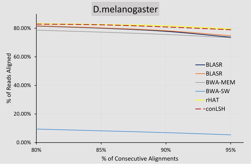
bioRxiv preprint first posted online Mar. 12, 2019; doi: http://dx.doi.org/10.1101/574467. The copyright holder for this preprint
  (which was not peer-reviewed) is the author/funder, who has granted bioRxiv a license to display the preprint in perpetuity.
                                 It is made available under a CC-BY-NC 4.0 International license.

                                       LSH                                                             conLSH

               0     1     2    3     4     5     6     7     8     9             0    1     2     3     4     5     6      7    8   9

                                 hLSH(2)=hLSH(5)=hLSH(8)=3
                                                                                                  hconLSH(1)=hconLSH(7)=0
                                                                                                  hconLSH(2)=hconLSH(8)=1

                                                                                      5
                     3

                                                                                      4
                     2

                                                                                      3
                                                                                      2
                     1

                                                                                      1
                     0

                                                                                      0

                                 LSH Table                                                         conLSH Table
                                          (a)                                                                (b)

Figure 1. Portrays the conceptual difference between Locality Sensitive Hashing and Context based Locality Sensitive
Hashing. Figure 1(a) shows that LSH places the balls of same color into the same slots of the hash table. The green balls from
positions 2, 5, and 8 are hashed into the 3rd slot of LSH Table. conLSH, on the other hand, groups the green balls from
positions 2 and 8 together (Figure 1(b)), keeping the ball from 5 at a different location in the hash table. The reason is that the
green balls at positions 2 and 8 share a common context of blue and red in both sides of them. Whereas, the ball from position
5 has a different context of two yellow balls in its left and right, which makes it hashed differently.

has huge memory footprint (13.70 Gigabytes for H. Sapiens dataset28 ) and produces large index file even with the default
parameter setting of k=13. Long SMRT reads facilitate the use of longer seeds for sensitive alignment and repeat resolution25 .
However, the excessive memory requirement restricts rHAT from increasing kmer size. Herein, we propose a novel concept of
Context based Locality Sensitive Hashing (conLSH) to align noisy PacBio data effectively within limited memory footprint.

    Hashing is a popular approach of indexing objects for fast retrieval. In conLSH, sequences are hashed together if they share
similar contexts. The probability of collision of two sequences is proportional to the number of common contexts between
them. The contexts play an important role to group sequences having noisy bases like PacBio data. The workflow of indexing
reference genome and alignment of SMRT reads using conLSH, is portrayed in the Figure 2. At the indexing phase, the
reference genome is virtually split into several overlapping windows. For each window, a set of conLSH values has been
computed and stored as a B-Tree index (for details refer Supplementary Note 1) to facilitate logarithmic index search. The
aligner hashes the SMRT reads using the same conLSH functions and retrieves the window-list from B-Tree index that resulted
into the same hash values as the read. This forms the list of candidate sites for possible alignment after extension. Finally, for
each read, the best possible alignment(s) are obtained by Sparse Dynamic Programming (SDP).
The combined hashed value, as shown in Fig. 2, captures contexts from K (concatenation factor) different locations, where

                                                                                                                                         2/11
bioRxiv preprint first posted online Mar. 12, 2019; doi: http://dx.doi.org/10.1101/574467. The copyright holder for this preprint
(which was not peer-reviewed) is the author/funder, who has granted bioRxiv a license to display the preprint in perpetuity.
It is made available under a CC-BY-NC 4.0 International license.
each context is of size 2 × λ + 1, (λ is the context factor, Refer Methods Section). This increases the seed length to resolve
repeats and thereby prevents false positive targets. Therefore, even if a kmer is repetitive, conLSH aligner can map it properly
with the help of its contexts. The problem occurs when the repeat regions are longer than the reads. However, this is very
unlikely due to the increased read length of SMRT data. The number of hash tables (L), context factor (λ ) and concatenation
factor (K) play an important role to make the aligner work at its best. An increase in λ and K, will make the aligner more
selective. Then, L should be sufficiently large to ensure that the similar sequences are hashed together in at least one of the L
hash tables2 . It may happen that a longer read could not be mapped to the reference genome by an end to end alignment. In that
case, conLSH has a provision of chimeric read alignment where a read is split and rehashed to find the candidate sites for each
split, and aligned accordingly.
SMRT Read 1
Window1 Window3 Windown
1. Windowing
ATTTCGGTCGCGTACCGTACGGATCAGGGAATA
ATTCGTTATCGGGTCCATTTCGGTCAAATTTAC
1. conLSH computation
h1 h2 h3 co
nt
Window 2 ex
ts
K=3 ize
Window i
size Repeat this
t ext
con L times Combined conLSH Value H
2. conLSH computation
GGTCATTTCGGTCGGTCAAATACCCTAAAACCTCTAAACCTAACTCA
h1 h2 h3 K=3 Search H in B-tree to retrieve
the window list
Repeat this
Combined conLSH Value H
L times
conLSH
2. Build target window list
Index
Insert hash value in B-Tree
ture
ruc
o d e st ree
n -T
of B
H1 H2 H3 Hn conLSH Value
3. Index tree formation
wl1 wl2 wl3 ... wln
window list
Obtain top M candidate
window list
3. Align to Ref genome
Best possible alignment(s)
by window extension and
SDP aligner
Read 1
Read 1
Reference Genome
(a) (b)
Figure 2. (a) describes the three different stages: Windowing, conLSH computation and Index tree formation of
conLSH-indexer. conLSH-aligner computes the hash value for the reads and uses the index tree build by conLSH-indexer to
map reads back to the reference genome. The worflow of conLSH-aligner is depicted in Fig.(b), which goes through the phases
of conLSH computation, Build target window list, and Alignment to reference genome.
Results
We have conducted exhaustive experiments on both simulated and real PacBio datasets to assess the performance of our
proposed conLSH based aligner. The result is demonstrated in three categories: i)Performance on Reference Genome Indexing,
ii)Results of SMRT read Alignments and iii)Robustness of conLSH aligner to different parameter settings. Five real (E.coli,
A.thaliana, O.sativa, S.cerevisiae, H.sapiens) and four simulated SMRT datasets were used to benchmark the performance of
conLSH and four other state-of-the-art aligners, rHAT28 , BLASR25 , BWA-MEM27 and BWA-SW26 . A detailed description
3/11bioRxiv preprint first posted online Mar. 12, 2019; doi: http://dx.doi.org/10.1101/574467. The copyright holder for this preprint
(which was not peer-reviewed) is the author/funder, who has granted bioRxiv a license to display the preprint in perpetuity.
It is made available under a CC-BY-NC 4.0 International license.
of the datasets along with their accession link is included in Supplementary Table 1. A brief manual for different working
parameters and a Quick Start guide can be found at Supplementary Note 3. The experiment has been conducted on an Intel R
CoreTM i7-6200U CPU @ 2.30GHz × 8(cores), 64-bit machine with 16GB RAM.
Performance on Reference Genome Indexing
Indexing of reference genome is the first step of the pipeline. The index file generated in this phase tries to encompass the
pattern lies in the entire genome, which is later used by the aligner to map the reads back to the reference. Table 1 portrays the
performance of conLSH-indexer in comparison with two other state-of-the-art methods, rHAT and BWA. BLASR is not listed
here, because it works better with BWT-index25 . We executed rHAT for two different parameter settings, rHAT1 with -l 11, -w
1000, -m 5, -k 13 (default settings) and rHAT2 with -l 8, -w 1000, -m 5, -k 15 (settings similar to conLSH).
Dataset E.coli H.sapiens A.thaliana S.cerevisiae O.sativa
Size(MB) Time(S) Size(MB) Time(S) Size(MB) Time(S) Size(MB) Time(S) Size(MB) Time(S)
conLSH 1.38 0.01 724.32 49 29.87 1 3.03 0.01 93.18 7
rHAT1 290 4 11755.34 785 742.84 35 316.91 3 1744.08 122
rHAT2 4317 49 15806.77 1166 4770.16 115 4343.47 50 5804 253
BWA 9.7 8.7 4523 3904 209 114.7 21.3 10.16 652.4 543.3
Table 1. The time required to produce the reference index and the index file size by three different methods for E.coli,
H.sapiens, A.thaliana, S.cerevisiae, and O.sativa genomes
It can be observed from Table 1 that conLSH is the fastest one to produce the reference index, and that is too of the least
size. conLSH yields a reduction of 94% in index size, while saving 93.7% of the time for H.sapiens genome, in comparison to
rHAT (default). The gain in time and index size attained by conLSH increases for rHAT2. BWA, on the other hand, produces
indexes of size smaller than that of rHAT, but at the cost of time.
Results of SMRT Read Alignments
We have used the PacBio P5/C3 release datasets respectively from H.sapiens, E.coli, S.cerevisiae, A.thaliana and O.sativa
(Please refer Supplementary Table 1 for details) genomes to extensively study the performance of proposed conLSH-aligner for
noisy and long SMRT reads. Table 2 summarizes the results for H.sapiens dataset by conLSH, rHAT, BWA-MEM, BWA-SW
and BLASR, in terms of time taken, percentage of the reads aligned and the peak memory footprint. The working parameters
of BWA-MEM, BWA-SW and BLASR, as found to be appropriate28 for PacBio data, is mentioned in the table. conLSH
operating at a default settings of -l 8, -w 1000, -m 5, - λ 2, -K 2, -L 1, generates patterns of length 16 (context size=2λ + 1=5
and concatenation factor (K)=2) assuming a gap of 3 bases between the contexts. To make rHAT comparable with conLSH, a
settings (rHAT2) with longer kmer (-k 15) has been used rather than the default kmer size of 13 (rHAT1).
Methods Working Parameters Time Taken (Sec) % of Reads Aligned Peak Memory Footprint (MB)
rHAT1 -l 11, -w 1000, -m 5, -k 13 210839 99.8 14562
rHAT2 -l 8, -w 1000, -m 5, -k 15 667280 100 15746
conLSH -l 8, -w 1000, -m 5, - λ 2, -K 2, -L 1 159888 99.8 4327
BLASR BWT 724304 99.7 8100
BLASR SA 848602 99.8 14700
BWA-MEM -x PACBIO 372782 99.7 5200
BWA-SW -b 5, -q 2, -r 1, -z 20 1145150 99.76 7100
Table 2. Performance of rHAT, conLSH, BLASR, BWA-MEM and BWA-SW for real PacBio H.sapiens P5/C3 release
Table 2 shows that conLSH aligns 99.8% reads of the real H.sapiens dataset in least time, producing a time gain of 24.2%
and 76% over rHAT1 and rHAT2 respectively. The smallest run-time memory requirement of 4.3GB, which is 70.3% less than
that of rHAT1, makes conLSH an attractive choice as SMRT aligner. The longer PacBio reads provide better repeat resolution
by facilitating larger kmer match. However, the huge memory requirement of 15.7GB, even at a kmer size of 15, makes rHAT
infeasible to work with longer stretches. Though, BWA-MEM , BWA-SW and BLASR yields lesser memory footprint in
comparison to rHAT, the performance is limited by the alignment speed. A similar scenario is reflected in Figure 3, when
studied with other PacBio datasets of E.coli, S.cerevisiae, A.thaliana and O.sativa. conLSH has been found to consistently
outperform the state-of-the-art methods in terms of memory consumption, while maintains a high throughput at the same time.
4/11bioRxiv preprint first posted online Mar. 12, 2019; doi: http://dx.doi.org/10.1101/574467. The copyright holder for this preprint
(which was not peer-reviewed) is the author/funder, who has granted bioRxiv a license to display the preprint in perpetuity.
It is made available under a CC-BY-NC 4.0 International license.
(a) E.coli PacBio Dataset (b) S.cerevisiae PacBio Dataset
(c) A.thaliana PacBio Dataset (d) O.sativa PacBio Dataset
Figure 3. Peak Memory footprint, % of Reads Aligned and Time Taken by rHAT1, rHAT2, conLSH, BLASR-BWT, BLASR-SA,
BWA-MEM, BWA-SW for four real PacBio datasets of E.coli, S,cerevisiae, A.thaliana, O.sativa genomes
Alignment on Simulated Datasets
In this section for simulated datasets, we have restricted our study to rHAT and conLSH only, as rHAT has been found to work
better28 than BWA and BLASR in terms of alignment speed and quality for SMRT reads. We used four different simulated
datasets, E.coli, S,cerevisiae, A.thaliana and D.melanogaster, originally generated to test the performance of rHAT28 using
PBSim29 with 1x coverage having average read length of 8000bp and 15% error probability (12% insertions, 2% deletions and
1% substitutions) resembling the PacBio P5/C3 dataset (Please refer Supplementary Table 1 for details).
The Table 3 describes the performance of rHAT1 (default settings), rHAT2 (settings similar to conLSH) in comparison with
the proposed conLSH-aligner for simulated datasets. It is evident that conLSH has the lowest memory footprint for all the
datasets. With similar kmer size, rHAT2 consumes 92% more space, on average, than conLSH. The speed of rHAT aligner is
achieved at the cost of huge memory requirement. The exhaustive hashing makes the search faster, but increases the index size.
In spite of that, conLSH works faster than rHAT2 for most of the datasets, as can be seen from Table 3, except D.melanogaster.
Though, rHAT1 works reasonably good in terms of memory footprint and alignment speed for these simulated datasets, it fails
to take the advantage of longer SMRT reads due to the small size of kmers. An exhaustive study on simulated datasets for
different working parameters of conLSH can be found at Supplementary Table 2.
5/11bioRxiv preprint first posted online Mar. 12, 2019; doi: http://dx.doi.org/10.1101/574467. The copyright holder for this preprint
(which was not peer-reviewed) is the author/funder, who has granted bioRxiv a license to display the preprint in perpetuity.
It is made available under a CC-BY-NC 4.0 International license.
Dataset Methods Working Parameters Time Taken (Sec) % of Reads Aligned Peak Memory Footprint (MB)
rHAT1 -l 11, -w 1000, -m 5, -k 13 6 94.8 294
E.coli sim rHAT2 -l 8, -w 1000, -m 5, -k 15 59 100 4225
conLSH -l 8, -w 1000, -m 5, - λ 2, -K 2, -L 1 15 100 85
rHAT1 -l 11, -w 1000, -m 5, -k 13 9 100 326
S.cerevisiae sim rHAT2 -l 8, -w 1000, -m 5, -k 15 85 100 4259
conLSH -l 8, -w 1000, -m 5, - λ 2, -K 2, -L 1 45 100 156
rHAT1 -l 11, -w 1000, -m 5, -k 13 89 100 849
A.thaliana sim rHAT2 -l 8, -w 1000, -m 5, -k 15 372 100 4781
conLSH -l 8, -w 1000, -m 5, - λ 2, -K 2, -L 1 337 99.9 574
rHAT1 -l 11, -w 1000, -m 5, -k 13 139 100 1054
D.melanogaster sim rHAT2 -l 8, -w 1000, -m 5, -k 15 223 98 4987
conLSH -l 8, -w 1000, -m 5, - λ 2, -K 2, -L 1 395 99 705
Table 3. Comparative study of Memory Requirement, % of Reads Aligned and Time Taken by rHAT and conLSH for four
different simulated datasets of E.coli, S,cerevisiae, A.thaliana and D.melanogaster genomes respectively
Quality of Alignment
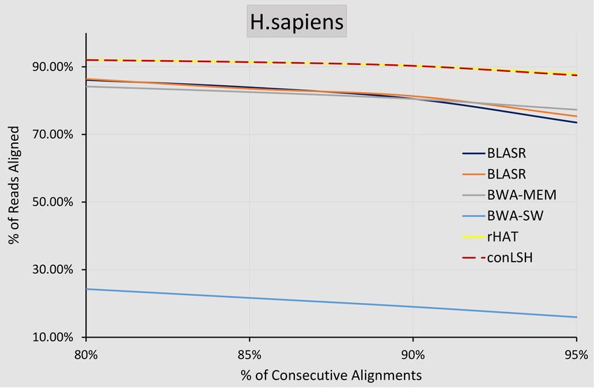
To assess the quality of the alignments, we have conducted an experiment to measure the number of reads aligned consecutively
by the respective aligners. Figure 4 plots the % reads aligned with a specific amount of continuity for real H.sapiens and
D.melanogaster datasets. It can be observed that conLSH has 92.02% of the aligned reads with 80%-consecutiveness. The
amount is almost similar for rHAT and gradually decreases for BWA-MEM, BLASR and BWA-SW. This this due to the fact
that after shortlisting the target sites for read mapping, conLSH adopts the same procedure of window expansion and SDP
based alignment as done by rHAT. This makes the alignment quality of rHAT and conLSH quite similar, which is reflected in
Figure 4.
(a) H.sapiens PacBio Dataset (b) D.Melanogaster PacBio Dataset
Figure 4. Reads aligned consecutively by different methods for the datasets, H.sapiens and D.melanogaster
Study of Robustness for different parameter values
To assess robustness of the proposed method, we have studied the performance of conLSH for different working parameters.
The result of conLSH indexer and aligner on subread m130928 232712 42213 of Human genome for different values of
concatenation factor (K), context size (2λ + 1) and number of hash tables (L), are comprehensively reported in Table 4. It is
clear that the size of the reference index is directly proportional with the number of hash tables (L). The parameters K and λ ,
on the other hand, decide the kmer size for pattern matching and therefore, have a strong correlation with the memory footprint
of the aligner. The parameters, K and λ together control the size of the BTree index in memory for storing the hash values
and the corresponding window lists. An increase in K and λ makes the aligner more selective in finding the target sites and
consequently, increases the sensitivity. To ensure a desired level of throughput, L should be sufficiently large so that the similar
sequences are hashed together into at least one of the L hash tables. Maintaining a trade-off between the memory footprint
and throughput, a settings of K = 2, λ = 2, L = 1 has been chosen as the default (marked as bold in Table 4). However, it is
6/11bioRxiv preprint first posted online Mar. 12, 2019; doi: http://dx.doi.org/10.1101/574467. The copyright holder for this preprint
(which was not peer-reviewed) is the author/funder, who has granted bioRxiv a license to display the preprint in perpetuity.
It is made available under a CC-BY-NC 4.0 International license.
needless to mention that the performance of conLSH does not change severely with the change of parameters. Please note that,
with λ = 0, the context size becomes 1 and the algorithm works as normal LSH based method without looking for any contexts
to match. It can be concluded from Table 4 that for a particular value of K and L, an increase in the context size enhances the
sensitivity of the aligned reads as well as the throughput of the aligner. A similar study with different working parameters for
four other real datasets has been included in Supplementary Table 3.
Concatenation Context Size L conLSH indexer conLSH aligner
Factor (K) 2×λ +1 Time(s) Hash size(MB) Time(s) %of Reads Aligned Peak Memory (MB)
2 1 1 46 724.32 341 97.9 3811
2 1 2 57 1448.65 424 95.7 4542
2 3 1 49 724.32 391 98.3 3813
2 3 2 56 1448.65 390 98.4 4521
2 5 1 49 724.32 444 99 4327
2 5 2 55 1448.65 505 99.1 5050
3 1 1 79 724.32 439 99 3799
3 1 2 62 1448.65 441 99.1 4518
3 3 1 49 724.32 452 99.1 3932
3 3 2 58 1448.65 468 99.2 4651
Table 4. Performance of conLSH with the change of K, L and λ for subread m130928 232712 42213 of H.sapiens dataset
Discussion
In this article, we have conceived the idea of context based locality sensitive hashing and deployed it to align noisy and long
SMRT reads. The strategy of grouping sequences based on their contextual similarity not only makes the aligner work faster, but
also enhances the sensitivity of the alignment. The result is evident from the experimental study on different real and simulated
datasets. It has been observed that larger seeds are helpful for aligning noisy and repetitive sequences25 . The combined hash
value, as obtained from the contexts of different locations of the sequence stream, makes conLSH work more accurately in
comparison to rHAT, a recently developed state-of-the-art method. Having a 32-bit hash value, the maximum possible kmer
size of rHAT is 16 (as, 232 = 416 ). The PointerList of rHAT stores links to all possible 4k hash values incurring a huge memory
cost. As a result, rHAT has a memory requirement of 13.7GB and 17.48GB with kmer size of 13 and 15 respectively for
H.sapiens dataset. The exponential growth of RAM space with the increase of kmer size prohibits rHAT from using larger seeds.
Moreover, rHAT generates 256 auxiliary files during indexing of reference genomes. This huge space constraint restricted the
utility of rHAT and demanded for a fast as well as memory efficient solution. conLSH is an effort in this direction. It efficiently
reduces the search space by storing the hash values and the corresponding window lists dynamically on demand. B-tree index
of the proposed aligner also facilitates efficient disk retrieval for huge genome, if could not be accommodated in memory. The
selection of context size (λ ) adds extra flexibility to the aligner. An increase in λ and K increases the seed size and makes the
aligner more sensitive. This mode of operation is specially suitable for aligning repetitive stretches. Therefore, conLSH can
serve as a drop-in replacement for current SMRT aligners.
conLSH also has some limitations to mention. The Sparse Dynamic Programming (SDP) based heuristic alignment is time
consuming and may lead to false positive alignments28 . As we have inherited the SDP based target site alignment from rHAT,
the shortcomings of it are also there in conLSH. Though, the default parameter settings work reasonably good for most of the
datasets studied, conLSH requires a understanding of context factor and LSH parameters in order to be able to use it. We have
future plan to automate the parameter selection phase of the algorithm by studying the sequence distribution of the dataset.
conLSH can be further enhanced by incorporating parallelization taking into account of the quality scores of the reads.
Methods
Nearest neighbor search is a classical problem of pattern analysis, where the task is to find the point nearest to a query from a
collection of d-dimensional data points. A less stringent version of exact nearest neighbor search is to find the R-nearest neigh-
bors, in which the algorithm finds all the neighbors within a certain distance R of the query. It can be formally defined as follows:
Definition 1. R-Nearest Neighbor Search:2
Given a set of n points X= {x1 , x2 , . . . , xn } in d-dimensional space Rd and a query point y, it reports all the points from the set
X which are at most R distance away from y, where R > 0.
7/11bioRxiv preprint first posted online Mar. 12, 2019; doi: http://dx.doi.org/10.1101/574467. The copyright holder for this preprint
(which was not peer-reviewed) is the author/funder, who has granted bioRxiv a license to display the preprint in perpetuity.
It is made available under a CC-BY-NC 4.0 International license.
Due to the “Curse of Dimensionality” the performance of most of the partitioning based algorithms, like kd-trees, degrades
for higher dimensional data. However, there are few exceptions30 where the authors have shown good results with priority
search k-means tree based algorithm. A solution to this problem is approximate nearest neighbor search. These approximate
algorithms return, with some probability, all points from the dataset which are at most c times R distance away from the query
object. The standard definition of c-approximate nearest neighbor search is:
Definition 2. c-approximate R-near Neighbor Search:2
Given a set of n points X= {x1 , x2 , . . . , xn } in d-dimensional space Rd and a query point y, it reports all the points x from the set
X where d(y, x) ≤ cR with probability (1 − δ ), δ > 0, provided that there exists an R-near neighbor of y in X, where R > 0 and
c > 1.
The advantage of using approximate algorithms is that they work very fast and the reported approximate neighbors are
almost as good as the exact ones2 . Locality Sensitive Hashing based approximate search algorithms are very popular for high
dimensional data. LSH works on the principle that the probability of collision of two objects is proportional to their similarity.
Therefore, after hashing all the points in the dataset, similar points will be clustered in the same or localized slots of the hash
tables. LSH is defined as:1
Definition 3. Locality Sensitive Hashing:
A family of hash functions H : Rd → U is called (R, cR, P1 , P2 )-sensitive if ∀x, y ∈ Rd
• if k x − y k≤ R, then PrH [h(x) = h(y)] ≥ P1
• if k x − y k≥ cR, then PrH [h(x) = h(y)] ≤ P2 , where, P1 > P2 .
We have proposed the following definitions and theories to develop the framework of Context based Locality Sensitive
Hashing(conLSH).
Definition 4. Context based Locality Sensitive Hashing (conLSH):
A family of hash functions H ∗ is defined as H ∗ : Rd+1 → U where the additional dimension denotes the context factor. H ∗
is called (R, cR, λ , P1∗ , P2∗ )-sensitive if ∀x, y ∈ Rd
• if k xλ − yλ k≤ R, then PrH ∗ [h∗ (x, λ ) = h∗ (y, λ )] ≥ P1∗
• if k xλ − yλ k≥ cR, then PrH ∗ [h∗ (x, λ ) = h∗ (y, λ )] ≤ P2∗ , where, P1∗ > P2∗ .
Here h∗ (x, λ ) is the context based locality sensitive hash function and xλ is the point x associated with a context of size
(2λ + 1), where λ is the context factor. Let x1 , x2 , . . . , xn and y1 , y2 , . . . , ym are two sequences on which conLSH is being applied.
Then, h∗ (xi , λ ) is actually a composition of (2λ + 1) standard LSH functions as defined below:
Definition 5. h∗ (xi , λ ):
h∗ (xi , λ ) = h(x(i−λ ) ) ◦ h(x(i−(λ −1) ) ◦ · · · ◦ h(xi ) ◦ h(x(i+1) ) ◦ · · · ◦ h(x(i+λ ) ), where 1 ≤ i ≤ n.
From now onwards, the context based LSH function h∗ (xi , λ ) is shortened as hλi . In the next subsection, we introduce the K
and L parameter values in connection with the concatenation of hash functions to amplify the gap between P1 and P2 .
Gap Amplification
As the gap between the probability values P1 and P2 is very small, several locality sensitive hash functions are usually
concatenated to obtain the desired probability of collision. This process of concatenation of hash functions to increase the
gap is termed as “gap amplification”. Let there be L hash functions, g1 , g2 , . . . , gL , such that g j is the concatenation of K
randomly chosen hash functions like, g j = (hλ1, j , hλ2, j , . . . , hλK, j ) for 1 ≤ j ≤ L. Therefore, the probability that g j (x) = g j (y)
(2λ +1)K
is at least P1 . Each point, x, from the database is placed into the proper slots of the L hash tables using the values
g1 (x), g2 (x), . . . , gL (x) respectively. Later when the query, y comes, we search though the buckets g1 (y), g2 (y), . . . , gL (y).
Note that larger values of K lead to larger gap between the LSH probabilities. As a consequence, the hash functions become
more conservative in estimating the similarity between points. In that case, L should be large enough to ensure that similar
points collide with the query at least once. The context factor λ should also be chosen carefully because if it is too large it will
overestimate the context, thereby making hash functions more stringent. A detailed theoretical discussion on the choice of the
parameters K, L, and λ is included in Supplementary Note 2.
8/11bioRxiv preprint first posted online Mar. 12, 2019; doi: http://dx.doi.org/10.1101/574467. The copyright holder for this preprint
(which was not peer-reviewed) is the author/funder, who has granted bioRxiv a license to display the preprint in perpetuity.
It is made available under a CC-BY-NC 4.0 International license.
Algorithm and Analysis
Algorithm 1 Indexing of Reference Genome using conLSH
Input: Let R be the Reference Genome 7: Place Wi in the g j (Wi ) th slot of the jth hash table,
K,L,λ are the conLSH parameters where g j (Wi ) = (hλ1, j ◦ hλ2, j ◦ · · · ◦ hλK, j )
context size=2λ + 1 hλk, j is randomly chosen from H ∗ along with a context
w=window size (default=2000bp)
of size (2λ + 1), 1 ≤ k ≤ K.
Output: conLSH index of R is stored in B-Tree
8: Insert the window position and the corresponding
1: R is split into n windows, (W1 ,W2 , . . . ,Wn ), each of size w,
conSH value in B-Tree Index.
having overlap of w/2 bp.
9: j ← j+1
|Wi | = w, for 1 ≤ i ≤ n
10: end while
2: i ← 1
11: i ← i+1
3: while i ≤ n do
12: end while
4: conLSH value will be computed for window Wi
13: The B-Tree with all window positions along with their
5: j←1
conLSH values forms the reference index.
6: while j ≤ L do
Algorithm 2 Alignment of PacBio Reads to the Reference Genome
Input: Long, noisy SMRT reads and the alignment scores 9: for each candidate window Ci , 1 ≤ i ≤ M do
(match, mismatch and gap penalties) 10: Ci window is further extended to obtain the probable
Output: Best possible alignment(s) for each read in the refer- alignment site as done in rHAT28 .
ence genome 11: Finally, the SDP-based heuristic alignment approach
1: for each PacBio read r do has been inherited from rHAT, where a directed acyclic
2: Compute the conLSH values for the L hash tables graph (DAG) is build to find the mapping.
3: j←1 12: end for
4: while j ≤ L do 13: If the read r could not be successfully aligned to any of
5: Place r in g j (r) th slot in the jth hash table, where g j the probable candidate sites, the algorithm tries to find
is the same conLSH function defined in Algorithm 1. chimeric read alignment. It splits a read into several fixed
6: Search B-Tree index for g j (r) to retrieve the window sized segments and the same procedure of conLSH com-
list that are mapped with the same hash value. putation and target location search is applied for each of
7: end while the segments.
8: Obtain M most frequent candidate windows from the 14: end for
window list.
Space Complexity
The space consumed by the algorithm is dominated by the hash tables and the data stored in it. Let there be a total of n
reads to be placed into L different hash tables. Therefore, the space requirement is =O(L × n)
=O(nρ · ln δ1 · n), See Supplementary Note 2.
=O(ln δ1 · nρ+1 )=O(nρ+1 )
Indexing Time:
For each sequence, L different hash values are computed for L hash tables. Each hash function is composed of (2λ + 1) × K
unit hash functions. Therefore, the time required to map a single read to its suitable positions in L different hash tables is
O((2λ + 1) · K · L)
Therefore, the total time requirement for n sequences is O((2λ + 1) · K · L · n)
=O((2λ + 1) · ( 2λ1+1 ) ln n1 · L · n), See Supplementary Note 2
ln P
2
ρ+1 ·ln n
=O( ln n1 · nρ 1
· ln · n)=O( n )
ln P δ ln P1
2 2
9/11bioRxiv preprint first posted online Mar. 12, 2019; doi: http://dx.doi.org/10.1101/574467. The copyright holder for this preprint
(which was not peer-reviewed) is the author/funder, who has granted bioRxiv a license to display the preprint in perpetuity.
It is made available under a CC-BY-NC 4.0 International license.
Query Time:
The search for target windows from the sequences that are hashed together with the query, is usually stopped after reporting
L0 = 3L candidates. This ensures a reasonably good result with constant error probability1 . In this case, the query time is
bounded by O(3L) = O(nρ · ln δ1 )=O(nρ ). However, if all the collided strings are checked, the query time can be as high as
θ (n) in the worst case. But, for many real data sets, the algorithm results in sublinear query time with proper selection of the
parameter values2 .
References
1. Indyk, P. & Motwani, R. Approximate nearest neighbors: towards removing the curse of dimensionality. In Proceedings of
the thirtieth annual ACM symposium on Theory of computing, 604–613 (ACM, 1998).
2. Andoni, A. & Indyk, P. Near-optimal hashing algorithms for approximate nearest neighbor in high dimensions. In
Communications of the ACM - 50th anniversary issue, 117–122 (ACM, 2008).
3. Datar, M., Immorlica, N., Indyk, P. & Mirrokni, V. S. Locality-sensitive hashing scheme based on p-stable distributions. In
Proceedings of the twentieth annual symposium on Computational geometry, 253–262 (ACM, 2004).
4. Gorisse, D., Cord, M. & Precioso, F. Locality-sensitive hashing for chi2 distance. Pattern Analysis Mach. Intell. IEEE
Transactions on 34, 402–409 (2012).
5. Ji, J. et al. Batch-orthogonal locality-sensitive hashing for angular similarity. Pattern Analysis Mach. Intell. IEEE
Transactions on 36, 1963–1974 (2014).
6. Ke, Y., Sukthankar, R. & Huston, L. Efficient near-duplicate detection and sub-image retrieval. In ACM Multimedia, vol. 4,
5 (2004).
7. Xia, H., Wu, P., Hoi, S. C. & Jin, R. Boosting multi-kernel locality-sensitive hashing for scalable image retrieval. In
Proceedings of the 35th international ACM SIGIR conference on Research and development in information retrieval, 55–64
(ACM, 2012).
8. Ryynanen, M. & Klapuri, A. Query by humming of midi and audio using locality sensitive hashing. In Acoustics, Speech
and Signal Processing, 2008. ICASSP 2008. IEEE International Conference on, 2249–2252 (IEEE, 2008).
9. Matei, B. et al. Rapid object indexing using locality sensitive hashing and joint 3d-signature space estimation. Pattern
Analysis Mach. Intell. IEEE Transactions on 28, 1111–1126 (2006).
10. Chakraborty, A. & Bandyopadhyay, S. A layered locality sensitive hashing based sequence similarity search algorithm for
web sessions. 2nd ASE Int. Conf. on Big Data Sci. Comput. Stanf. Univ. CA, USA (2014).
11. Hachenberg, C. & Gottron, T. Locality sensitive hashing for scalable structural classification and clustering of web
documents. In Proceedings of the 22nd ACM international conference on Conference on information & knowledge
management, 359–368 (ACM, 2013).
12. Vijayanarasimhan, S., Jain, P. & Grauman, K. Hashing hyperplane queries to near points with applications to large-scale
active learning. Pattern Analysis Mach. Intell. IEEE Transactions on 36, 276–288 (2013).
13. Buhler, J. Efficient large-scale sequence comparison by locality-sensitive hashing. Bioinformatics 17, 419–428 (2001).
14. Chakraborty, A. & Bandyopadhyay, S. Ultrafast genomic database search using layered locality sensitive hashing. In Fifth
International Conference on Emerging Applications of Information Technology (IEEE, 2018).
15. Berlin, K. et al. Assembling large genomes with single-molecule sequencing and locality-sensitive hashing. Nat.
biotechnology 33, 623–630 (2015).
16. Rhoads, A. & Au, K. F. PacBio sequencing and its applications. Genomics, proteomics & bioinformatics 13, 278–289
(2015).
17. Ardui, S., Ameur, A., Vermeesch, J. R. & Hestand, M. S. Single molecule real-time (SMRT) sequencing comes of age:
applications and utilities for medical diagnostics. Nucleic acids research 46, 2159–2168 (2018).
18. Ye, C., Hill, C. M., Wu, S., Ruan, J. & Ma, Z. S. DBG2OLC: efficient assembly of large genomes using long erroneous
reads of the third generation sequencing technologies. Sci. reports 6, 31900 (2016).
19. Khiste, N. & Ilie, L. HISEA: Hierarchical seed aligner for pacbio data. BMC bioinformatics 18, 564 (2017).
20. Roberts, R. J., Carneiro, M. O. & Schatz, M. C. The advantages of SMRT sequencing. Genome biology 14, 405 (2013).
21. Ye, C. & Ma, Z. S. Sparc: a sparsity-based consensus algorithm for long erroneous sequencing reads. PeerJ 4, e2016
(2016).
10/11bioRxiv preprint first posted online Mar. 12, 2019; doi: http://dx.doi.org/10.1101/574467. The copyright holder for this preprint
(which was not peer-reviewed) is the author/funder, who has granted bioRxiv a license to display the preprint in perpetuity.
It is made available under a CC-BY-NC 4.0 International license.
22. Li, H. & Durbin, R. Fast and accurate short read alignment with burrows–wheeler transform. Bioinformatics 25, 1754–1760
(2009).
23. Langmead, B. & Salzberg, S. L. Fast gapped-read alignment with bowtie 2. Nat. methods 9, 357 (2012).
24. Langmead, B., Trapnell, C., Pop, M. & Salzberg, S. L. Ultrafast and memory-efficient alignment of short dna sequences to
the human genome. Genome biology 10, R25 (2009).
25. Chaisson, M. J. & Tesler, G. Mapping single molecule sequencing reads using basic local alignment with successive
refinement (BLASR): application and theory. BMC bioinformatics 13, 238 (2012).
26. Li, H. & Durbin, R. Fast and accurate long-read alignment with burrows–wheeler transform. Bioinformatics 26, 589–595
(2010).
27. Li, H. Aligning sequence reads, clone sequences and assembly contigs with BWA-MEM. arXiv preprint arXiv:1303.3997
(2013).
28. Liu, B., Guan, D., Teng, M. & Wang, Y. rHAT: fast alignment of noisy long reads with regional hashing. Bioinformatics
32, 1625–1631 (2015).
29. Ono, Y., Asai, K. & Hamada, M. Pbsim: Pacbio reads simulator—toward accurate genome assembly. Bioinformatics 29,
119–121 (2012).
30. Muja, M. & Lowe, D. G. Scalable nearest neighbor algorithms for high dimensional data. Pattern Analysis Mach. Intell.
IEEE Transactions on 36, 2227–2240 (2014).
Author contributions statement
A.C. conceived the idea, carried out the work, wrote the main text, prepared the Figures and the software tool for conLSH. S.B.
planned the work, provided laboratory facilities and wrote the manuscript. Both authors reviewed the manuscript.
Additional information
Competing financial interests: The authors declare no competing financial interests.
Acknowledgment
SB acknowledges JC Bose Fellowship Grant No. SB/SJ/JCB-033/201.6 dated 01/02/2017 of DST, Govt. of India and DBT
funded project Multi-dimensional Research to Enable Systems Medicine: Acceleration Using a Cluster Approach for partially
supporting the study. A part of this work was done when SB was visiting ICTP, Trieste, Italy.
11/11You can also read