Contrasting structural complexity differentiate hunting strategy in an ambush apex predator
←
→
Page content transcription
If your browser does not render page correctly, please read the page content below
www.nature.com/scientificreports
OPEN Contrasting structural complexity
differentiate hunting strategy
in an ambush apex predator
Milan Říha1*, Karl Ø. Gjelland2, Vilém Děd1, Antti P. Eloranta3,5, Ruben Rabaneda‑Bueno1,
Henrik Baktoft4, Lukáš Vejřík1, Ivana Vejříková1, Vladislav Draštík1, Marek Šmejkal1,
Michaela Holubová1, Tomas Jůza1, Carolyn Rosten5, Zuzana Sajdlová1, Finn Økland5 &
Jiří Peterka1
Structural complexity is known to influence prey behaviour, mortality and population structure,
but the effects on predators have received less attention. We tested whether contrasting structural
complexity in two newly colonised lakes (low structural complexity lake—LSC; high structural
complexity—HSC) was associated with contrasting behaviour in an aquatic apex predator, Northern
pike (Esox lucius; hereafter pike) present in the lakes. Behaviour of pike was studied with whole-lake
acoustic telemetry tracking, supplemented by stable isotope analysis of pike prey utilization and
survey fishing data on the prey fish community. Pike displayed increased activity, space use, individual
growth as well as behavioural differentiation and spent more time in open waters in the LSC lake.
Despite observed differences between lakes, stable isotopes analyses indicated a high dependency
on littoral food sources in both lakes. We concluded that pike in the HSC lake displayed a behaviour
consistent with a prevalent ambush predation behaviour, whereas the higher activity and larger space
use in the LSC lake indicated a transition to more active search behaviour. It could lead to increased
prey encounter and cause better growth in the LSC lake. Our study demonstrated how differences in
structural complexity mediated prominent changes in the foraging behaviour of an apex predator,
which in turn may have effects on the prey community.
The composition of biotic assemblages is heavily influenced by habitat heterogeneity arising from both abiotic
and biotic components. Much focus has been given to the role that habitat complexity plays in structuring and
functioning at the population level, both in aquatic and terrestrial ecosystems1–3. The presence of varied structures
increases environmental heterogeneity and the range of available potential h abitats4, and by providing shelter
for prey or cover for predators structures have a crucial role in predator–prey interactions5. Physical structures,
either biotic or abiotic, may also provide suitable substrate for primary producers, filtering organisms etc., and
thus increase the food availability for p redators5.
Submerged macrophytes are among the main structuring components in freshwater ecosystems. Macrophytes
can substantially alter the behaviour of both prey and predators (e.g.5–7) via affecting predator–prey detection,
encounter and c atchability8. Some predators can alter their foraging behaviour and activity by switching between
ambush and active pursuit9–12 depending on the presence/absence of macrophytes. This ability is species-specific
and it has been documented in various groups of invertebrates6,12 and fish9,11, where it has implications for hunt-
ing success. Predators able to shift their foraging strategies may be able to maintain the total number of prey
captures as the yield of their favoured foraging strategy is r educed10–12. However, a switch in activity and foraging
behaviour to maintain prey consumption does not necessarily imply maintained predator growth and fitness,
as higher activity costs might not be balanced by the energy gain, and thus be less efficient6. The most beneficial
strategy will obviously be influenced by the rewards of the alternative strategies.
Besides the inherent ability of some species to modify foraging mode, recent research has revealed that
there may be large individual variation in how these behavioural traits are e xpressed13,14. Such variability may
be explained by sex-specific differences and individual variation in genetic and life-history t raits13,14, some
1
Biology Centre of the Czech Academy of Sciences, Institute of Hydrobiology, České Budějovice, Czech
Republic. 2Norwegian Institute for Nature Research (NINA), Tromsö, Norway. 3Department of Biological and
Environmental Science, University of Jyväskylä, Jyväskylä, Finland. 4National Institute of Aquatic Resources,
Technical University of Denmark (DTU Aqua), Vejlsøvej 39, 8600 Silkeborg, Denmark. 5Norwegian Institute for
Nature Research (NINA), Trondheim, Norway. *email: milan.riha@hbu.cas.cz
Scientific Reports | (2021) 11:17472 | https://doi.org/10.1038/s41598-021-96908-1 1
Vol.:(0123456789)
www.nature.com/scientificreports/
individuals may be more risk-prone than others, individual behaviour may be modified by social h ierarchies15,
or individuals may get more skilled and effective at one foraging tactic at the expense of other tactics15,16. More-
over, individual variation in foraging behaviour can also be linked with environmental complexity. Higher
inter-individual dietary variation (directly connected with foraging behaviour) was found under low structural
complexity, fostered by competition for macrophyte stands among individuals17,18. Although many predators
may be able to change foraging mode, many of these mechanisms suggest individual foraging specialization to
a specific foraging m ode15.
Apex predators can potentially modify ecosystem structure and this ability is tightly linked with structural
complexity in freshwater e cosystems19. Intraspecific variation in predator behaviour can determine prey abun-
dance, community composition and trophic cascades20. Understanding apex predator behaviour and its variability
in relation to structural complexity is therefore important to better understand their ability to cope with and/or
elicit ecosystem changes, as well as the environmental drivers of phenotypic plasticity.
Research on behavioural responses of predators to changes in structural complexity has been carried out
mainly at the species level in laboratory conditions or on small-scale experimental set-ups6,9–12. Such conditions
may be unsuitable for large predators or they could lead to important behavioural traits being ruled out21. Data at
the natural scale is sparse and fragmented, and our understanding of aquatic apex predator behaviour in natural
conditions is still highly insufficient. The development of high-resolution tracking t echniques22 now gives the
opportunity to explore behaviour with unprecedented spatiotemporal resolution that could bring new insights
into predator behaviour and their interaction with the environment23.
To test the effect of structural complexity on predator behaviour in natural conditions, we selected Northern
pike (Esox lucius) as a model species. Pike is considered as an important model organism for identifying causes
and consequences of phenotypic variation at the level of individuals and populations as well as for investigating
community processes24. It is a freshwater apex predator typically associated with structurally complex habitats,
often used as a classic example of a “sit-and-wait" ambush predator, and widely distributed in lakes and rivers
across the Holarctic r egion25,26. Pike is a voracious forager with a wide variety of fish and other prey types and
its introduction can have major impacts on fish species composition25,27. Recent research has revealed that pike
can utilize a wider range of habitats, show active hunting in open water areas, and migrate many k ilometres28–30.
In some freshwater ecosystems, pike show behavioural types that differ in their level of activity and selection of
habitat types31. Most seem to be strongly associated with structurally complex habitats, but this may also vary with
season and ontogeny32. These findings suggest that pike have the capability for individual plasticity in habitat use
and that differences in structural complexity may alter its foraging behaviour as a result of individual foraging
specialization. On the other hand, some experimental studies indicate only minor effects of macrophyte density
on pike behaviour9, and there is so far no evidence for how habitat complexity may alter the species’ behaviour
in natural conditions.
We addressed the question of how pike behaviour changes with contrasting structural complexity by tracking
pike with very high spatiotemporal resolution in two newly created post-mining lakes. The lakes have similar
morphological and environmental parameters, but highly different submerged macrophyte structural complex-
ity (low and high structural complexity, respectively LSC lake and HSC lake). Pike behaviour was investigated
by examining habitat use and activity (telemetry), food availability in different habitats (gillnet and acoustic
sampling of fish community), long-term diet (stable isotope analysis, SIA) and individual growth in tracked
pike (scale analysis). We hypothesised that (1) space use (horizontal and vertical) will be inversely related to
habitat complexity; (2) pike activity is inversely related to structural complexity; (3) the pelagic habitat and food
resources will be more important in the lake with lower habitat complexity; (4) individual behavioural traits are
consistent over time, but between-individual variation is higher in LSC lake; (5) growth is lower in the LSC lake,
as activity costs are expected to be higher.
Material and methods
Study lakes. The study was conducted in two water bodies created after aquatic restorations of mining
pits, Lakes Milada (2.5 km2, high structural complexity; 50° 39′ N, 13° 58′ E) and Most (3.1 km2, low structural
complexity lake; 50° 32′ N, 13° 38′ E), in the Czech Republic (Fig. 1). Aquatic restoration took place from 2001
to 2010 in Milada and from 2008 to 2014 in Most. Both lakes are medium-sized (surface area = 252 and 311
hectares, respectively), relatively deep (Zmean = 16 and 22 m, Zmax = 25 and 75 m), oligotrophic (mean summer
total phosphorus < 10 and < 5 μg/L) and the Secchi depth varies between 3–10 m in Milada and 7–10 m in Most
lake. The deeper Most has a well-oxygenated water column down to 50 m depth, whereas in Milada the profun-
dal zone suffers from poor oxygen conditions below 20 m depth in summer17.
Macrophyte sampling was carried out prior to the study in September 2014 and May 2 01533. Macrophytes
were dense only in the HSC lake where they covered 60–91% of 0–12 m deep inshore areas. In the LSC lake,
there was only a sparse macrophyte coverage of 0.1–1.6% at 0–3 m depth. Dominant macrophyte species in both
lakes were Potamogeton pectinatus, Myriophyllum spicatum and Chara sp.
Both lakes had similar fish community compositions. Roach (Rutilus rutilus) and perch (Perca fluviatilis)
were dominant in both lakes, while ruffe (Gymnocephalus cernua), tench (Tinca tinca), European catfish (Silurus
glanis), Northern pike and pikeperch (Sander lucioperca) were less abundant34. In addition, pelagic planktivorous
maraena whitefish (Coregnus maraena) were present in the LSC lake.
Stocking of predatory species including pike were performed in both lakes for biomanipulation purposes.
Stocking of pike was performed after filling of the lakes as a biomanipulation measure to improve and maintain
high water quality. In HSC lake, young-of the-year pike were stocked in 2005 and 1–2 year old pike in 2005,
while in LSC lake over 1-year old pike were stocked in years 2011–2013 (Detail information in Supplementary
material1 Tab. A1). Stocked pike came from various breeding ponds in the Central Bohemia region.
Scientific Reports | (2021) 11:17472 | https://doi.org/10.1038/s41598-021-96908-1 2
Vol:.(1234567890)
www.nature.com/scientificreports/
Figure 1. Locations and bathymetric maps of investigated lakes and positions of telemetry systems. Dots
represent positions of each telemetry receiver and stars positions of temperature loggers. The map created using
the Open Source QGIS version 3.18 (https://qgis.org/en/site/).
The pike populations were monitored long-term in both lakes and all captured pike were PIT tagged and
released back in to the lake (more details are given in35). The population size estimate (based on recaptures) was
around 220 individuals (size range 60–120 cm) in HSC lake in years 2014–2016. Low recaptures numbers did
not allow making asimilar population size estimate in LSC lake. By comparing efforts and catches in both lakes,
we estimated that population in LSC lake accounted for only 30–40% of that in HSC lake population (Vejřík L.,
unpublished data).
Telemetry system. Two separate MAP positioning systems (Lotek Wireless Inc., Canada) were deployed
in the HSC and LSC lakes to track tagged fish (see below). The systems consisted of 91 receivers (Lotek Wireless
Inc., WHS3250; 44 receivers in HSC lake, and 47 receivers in the LSC lake) deployed in arrays with distances
between the 3 nearest receivers ranging from 203 to 288 m (mean 251 ± 18 m) in the HSC lake and 191 to 341 m
(mean 264 ± 33 m) in LSC lake (Fig. 1). The exact position of deployed receivers was measured using a high-
precision GNSS-unit (Trimble Geo7x with a cm-precision RTK-service). Depth of receivers varied between 4.5
and 5.5 m. According to range testing done prior to the study, in these lakes (September 2014), such setting of
receiver arrays should provide full coverage of both lakes under appropriate environmental conditions. Moni-
toring of the system accuracy was achieved by 20 stationary reference tags (10 tags in each lake; Lotek Wireless
Inc., Canada, model MM-M-16-50-TP, burst rate 25 secs), located in 4 locations in each lake (2 open water loca-
tions at depths of 1, 5 and 13 m, and 2 nearshore locations at depths of 1 and 3 m). Further, testing of accuracy
was performed by reference tags dragged below a boat after the deployment and before the final retrieval of the
telemetry system (further information on positioning error are given in the Supplementary material 2). The sys-
tems were installed from April 2015 to March 2016 and the data was manually downloaded every two months.
The period targeted in this study lasted from 27 May 2015 to 10 October 2015 to cover the summer period with
the highest fish activity and development of macrophytes.
Fish tagging. A total of 30 pike individuals (15 in each lake) were captured by electrofishing (23 individu-
als), long-lines (6 individuals) and angling (1 individual). Mean total body length/mass was 79 cm/4.13 kg for
the HSC lake and 86 cm/4.15 kg for the LSC lake, respectively (more details in Table 1). After capture, pike were
anaesthetized by 2-phenoxy-ethanol (SIGMA Chemical Co., USA, 0.7 ml L−1, mean time in anaesthetic bath was
3.75 min), measured, weighed and tagged. A 1–1.5 cm long incision was made on the ventral surface posterior
to the pelvic girdle and the transmitter (Lotek Wireless Inc., MM-M-11-28-PM, 65 × 28 mm, mass in air of 13 g,
including pressure and motion sensors, burst rate 25 s, tag weight ranged between 0.1 and 1.7% of fish body
weigh; Table 1) was inserted through the incision and pushed forward into the body cavity. The incision was
closed using two independent sutures. Mean surgery time was 2.8 min. In addition, scales for age determina-
tion and stable isotope analysis (see below) were taken during anaesthesia. All pike were released immediately
after recovery from anaesthesia on the same location in each lake regardless of their capture location. Fish were
captured and tagged between 5 and 10 May 2015.
Scientific Reports | (2021) 11:17472 | https://doi.org/10.1038/s41598-021-96908-1 3
Vol.:(0123456789)
www.nature.com/scientificreports/
Ratio of tag weight to
Total length(cm)/Weight(kg) body weigh (%)
Lake No. tagged/analyzed Mean SD Min Max Mean Min Max
LSC 15/13 86.3/4.2 11.4/1.8 63.5/1.5 103.5/7.5 0.5 0.1 1.7
HSC 15/12 78.9/4.1 17.6/3.4 52/0.8 115/14.2 0.4 0.2 0.7
Table 1. Description of tracked pike in both study lakes.
Macrophyte sampling. To obtain an assessment of macrophyte assemblage and coverage, two SCUBA
divers visually assessed macrophyte occurrence along 25 (HSC lake) and 26 (LSC lake) transects at the end of
June and the beginning of September 2015. Sampling considered both aquatic plants as well as submerged dead
terrestrial plants (only present in the LSC lake). Transects were situated from the shore to a depth of 12 m or
deeper when macrophytes were present there. The coverage of each macrophyte species, the uncovered bottom
area, the percentage composition of each species and maximum and minimum height of each macrophyte spe-
cies were measured at 1 m depth intervals. The height of macrophytes was measured using a measuring tape.
Dead flooded terrestrial plants were mostly European elder Sambucus nigra and thus categorized as a single
group. Structural Complexity Index (hereafter referred to as SCI) in each lake was calculated to compare habitat
complexity between lakes and its development during the study period. Calculation of SCI was based on infor-
mation from the 25 and 26 (HSC and LSC lakes, respectively) scuba diver macrophyte assessment transects
(see above). Species coverage and macrophyte height were both considered for calculation of the index. Species
coverage and macrophyte height along each transect were georeferenced in a GIS-environment, and overlaid the
bathymetric map for the lake. Height of macrophytes was discretized into 100 bins (from 0 to 200 cm by 2 cm)
and coverage was discretized into 100 bins by 1%. The structural complexity index SCI was then defined as dis-
cretized height multiplied by discretized coverage. This gave a SCI range from 0 (no occurrence of macrophytes)
to 10 000 (macrophyte coverage 100% and height ≥ 2 m).
Temperature and oxygen measurement. To obtain abiotic parameters which can drive pike spatial
istribution36,37, we monitored water temperature and oxygen concentration in both lakes. Water temperature
d
was monitored using 60 data loggers (Onset, USA, HOBO Pendant temp/light 64 K). Data loggers were placed
at two sites in each lake in order to cover east/west (HSC lake) and south/north (LSC lake) gradients (Fig. 1).
At each site, data loggers were attached to a rope in 1 m intervals spanning from the surface to 13 m (14 data
loggers) with one extra data logger located at a depth of 20 m. The rope was tied to a floating buoy anchored at
22 m depth. This setup ensured both dense coverage in depths of rapid temperature change and, with a measure-
ment interval of 5 min, high spatiotemporal resolution of the temperature profile. Oxygen concentration was
measured in each lake (once a month in the HSC lake, and once during the observed period in the LSC lake)
by calibrated YSI 556 MPS probe (YSI Incorporated, USA). Measurements were performed close to the western
(HSC lake) or northern (LSC lake) data logger station (Fig. 1).
Fish community sampling. To obtain data of pike prey distribution, we performed spatially stratified
fish community sampling by gillnet and hydroacoustic surveys. Gillnet surveys were conducted in September
2014 and 2015 at two localities in each lake in benthic habitats and one central locality in each lake for pelagic
habitats, using 30 m long standard European multi-mesh g illnets38. At each locality in each lake, one series of
three survey nets were set in the benthic and pelagic habitats at depths 0–3, 3–6, 6–9 and 9–18 m. In the deeper
LSC lake, series of three survey nets were also set at depths 18–24, 24–30 and > 30 m. Benthic and pelagic gillnets
were 1.5 m and 3 m high, respectively. Gillnets were set overnight, i.e. installed 2 h before sunset and lifted 2 h
after sunrise39. Only catches of fish older than young-of-the-year were considered for this study. YOY fish were
excluded as their density can be largely underestimated in gillnet surveys40. Moreover, Vejřík et al.35 found only
prey fish larger than 10 cm in the stomachs of pike caught from both study lakes. Catches were expressed as catch
per unit of effort measured as number of fish caught per 1000 m2 gillnet area per night (NPUE), and as kilogram
fish 1000 m−2 night−1 (BPUE).
The acoustic surveys were performed both during the day and night, using a calibrated Simrad EK 60 echo-
sounder operating at frequency of 120 kHz and following a pre-set zig-zag cruise track. The transducer was
mounted 0.2 m below water surface, beaming vertically downwards. Recorded data were analysed using Sonar5-
Pro software version 6.0.341, using a Sv-threshold of − 62 dB (thresholded at 40 logR) and a target strength (TS)
threshold of − 56 dB (corresponding to fish with an approximate total length of 4 c m42). Shoals were detected
manually while fish tracking was used for individual fish. The following settings were used in the Sonar5-Pro
auto-tracking tool to select fish tracks: minimum track length (MTL), maximum ping gap (MPG) and verti-
cal range gating. MTL was set to 3 echoes, MPG was set to 1 and vertical gating to 0.15 m for the whole water
column. Only areas deeper than 5 m were included in further analysis. The relative fish density was calculated
for shoals (shoals ha−1) and individual fish (ind. ha−1) using the number of shoals or fish related to the surveyed
area (calculated from the wedge formed by the distance, the range and the opening angle). The analysed water
column was divided into depth layers (1 m thick, from 5 m below the surface to the bottom).
Data processing. Positions of individual fish were calculated using a proprietary post-processing software
UMAP v.1.4.3, based on multilateration of the time-difference-of-arrival (TDOA) of the acoustic signal received
Scientific Reports | (2021) 11:17472 | https://doi.org/10.1038/s41598-021-96908-1 4
Vol:.(1234567890)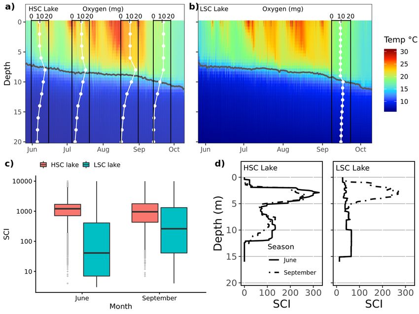
www.nature.com/scientificreports/
Raw positions q-positions
Lake Mean Min Max Sum Mean Min Max Sum
LSC 68,745 6301 116,333 893,685 6429 1370 10,818 83,581
HSC 116,201 49,211 198,881 1,394,416 7568 3899 12,581 90,819
Table 2. Yield of positions gathered by positioning systems in studied lakes (mean for all individuals, range
among individuals and total sum of all gather positions) and calculated 15-min q-positions.
at different telemetry loggers (Lotek Wireless Inc., Newmarket, Ontario, Canada). Positions calculated using
UMAP software can contain position duplicates and the use of TDOA for positioning implies large errors in a
proportion of the position estimates43. Therefore, a position filter was applied in order to remove duplicate posi-
tions and positions with large errors. A detailed description of the filtering procedure is given in the SM1 (sec.
Filtering of positions estimated by the U-MAP software). The position estimates (unfiltered and filtered) and
depth profiles of each individual fish was visually inspected. If both horizontal and vertical locations became
constant without latter movement, this individual was considered dead or expelling the tag (2 ind. in the LSC
lake and 3 ind. in the HSC lake) and removed from further analyses.
The detection probability of transmitter detection and thus horizontal positioning changed over time and
space due to underwater structures and thermal stratification. Numbers of position estimates for each individual
ranged from 0 to 2884 per day (from 0 to 83% of possible number of position estimates). In order to reduce
potential bias resulting from the varying positioning rate44, the individual data was regularized by calculating
mean position for every 15-min interval (q-position hereafter). The q-position mean depth was calculated as
the 15-min mean depth for each detected transmission with sensor depth reading. Since this did not require
trilateration, the q-position time series could have a depth value without having a position estimate. This gave
a maximum of 96 q-positions per day for each individual. If no position estimate was obtained within a 15-min
interval, the q-position was interpolated between q-positions close in time if several conditions were fulfilled; (a)
the time difference between the two q-positions used for interpolation (last before and first after the interval(s)
to be interpolated) had to be shorter than 2 h, (b) the distance between these q-positions was less than 100 m,
and (c) the depth difference between the q-positions was less than 2 m. Under such conditions, we assumed that
the fish movement was limited between the q-positions used for interpolation (likely due to resting in an area
with poor positioning coverage), and that linear interpolation in order to regularize the time series was therefore
justified. For each position estimate, distance to bottom was calculated as the bottom depth at that position sub-
tracted by the sensor depth. Distance to bottom for each q-position was calculated as the mean of each distance
to bottom estimate within the 15-min interval. Individual and total yield of positions and calculated q-positions
during the study period is given in Table 2.
Depth of fish was measured by an internal tag sensor and transmitted together with an tag identification.
Therefore, to get depth of fish, only detection of a single receiver was required (not three as for location of a
horizontal position). Depth location was, therefore, obtained in much higher detail than fish horizontal location
(fewer gaps). To synchronize depth and position with horizontal position, we calculated mean depth for the same
15-min intervals as we used for calculation of mean horizontal position from receiver detections at that interval.
Extent of horizontal area use was calculated using a 95% kernel utilization distribution (hereafter referred to
as dH-KUD). dH-KUD was calculated for each day and individual separately and only for days with more than
12 daytime and 12 night-time q-positions. Night-time and daytime were defined as one hour after/prior to civil
twilight periods39. Exact time of sunset and sunrise in each day was calculated using R-package “maptools”45 and
dH-KUD was calculated using R-package “adehabitatHR”46. Parameters required for calculation of dH-KUD
were set as follows:a simplified lake shape polygon was used as a boundary, a raster of a lake with a cell dimen-
sion of 10 × 10 m was used as a grid and the smoothing parameter h was set to value of 50. The extent of vertical
movement was evaluated separately. Vertical space use (hereafter referred to as dV-KS) was calculated as a one-
dimensional kernel estimate (95%) of Gaussian density function with the smoothing bandwidth parameter set
to 0.4 fitted on distribution of utilized depths.
Activity of fish was calculated as horizontal swimming speed (expressed in body lengths per second, BL * s −1)
and vertical swimming speed (depth change per second, m * s−1) between two consecutive q-positions.
To test the importance of an open water habitat for pike in both lakes, the proportion of time spent in open
water was calculated (TOW). Each q-position was assigned to be either in the benthic (distance < 5 m from the
bottom) or in the open water habitat (≥ 5 m from the bottom).
Daily water temperature and day length were abiotic factors considered to potentially drive pike behaviour
in lakes36,37,47. Daily water temperature was calculated as the mean temperature from measurement of all data
loggers at depths 0–3 m for each date during the study, separately for each lake. This parameter reflects both rapid
daily and gradual seasonal temperature changes. Day length was calculated as time between sunrise and sunset.
Stable isotopes and growth. Stable isotopes are widely used in studies of food-web structure and func-
tion, as well as individual specialization among consumer populations48,49. Here, we used stable carbon (δ13C)
and nitrogen (δ15N) isotopes to estimate the relative reliance of individual pike on littoral carbon (food) resources
(hereafter abbreviated as littoral reliance, LR). The LR estimates were calculated using the two-source isotopic
mixing model described in P ost50, where the δ13C value of a consumer (measured from the outermost annual
ring of pike scales) is compared to those of littoral and pelagic isotopic end-members. We used δ13C values of
Scientific Reports | (2021) 11:17472 | https://doi.org/10.1038/s41598-021-96908-1 5
Vol.:(0123456789)
www.nature.com/scientificreports/
littoral macrophytes and benthic algae, and pelagic particulate organic matter (POM) as the littoral and pelagic
isotopic end-members, respectively, because some pike individuals and herbivorous prey fishes had consider-
ably higher δ13C values than littoral benthic invertebrates. For more details of sample collection and preparation
for stable isotope analyses, see the previous studies of predatory35 and generalist17 fishes in the two study lakes.
Age determination and growth calculation for each individual were conducted using scale reading. Three
scales were read for each individual, results were then averaged and used for back-calculation of size-at-age of
each individual using the Fraser–Lee Equation51. Only the body increment during the year prior to tagging was
used to test for the correlation of individual growth with the rates of horizontal and vertical movement, since
this was the growth increment most relevant to the activity and body size during the study year.
Statistical analyses. Behavioural traits and use of the pelagic zone. The response variables analyzed were
horizontal area use (dH-KUD), vertical space use (dV-KS), daily mean depth (hypothesis i); horizontal activity,
vertical activity (hypothesis ii); and time spent in open water (TOW, hypothesis iii); all of which could be as-
sociated with either a foraging or cover context. To test whether individuals from both lakes exhibited consistent
behavioural differences across time we fitted a series of random-effects models and selected the best one based
on Akaike Information Criterion (AIC, hypothesis iv). These models included a different set of covariates previ-
ously selected through Random Forest (hereafter RF) regression analysis52 using the R package randomForest 53.
RF is suitable for the identification of relevant interactions between variables with low to negligible effects in
isolation (further description in SM1, sec. Identifying interactions with Random Forest), and thus it would allow
us to constraint both the number and potential interactions between them.
For the analysis of dH-KUD, dV-KS, mean depth horizontal activity and vertical activity we first fitted full
random-intercepts and random-slopes mixed-effects models (LMMs)54,55 with Gaussian error distribution using
the package nlme54. These models all include the same relevant predictors and interactions from the RF analysis,
which yielded quite consistent results between the analyzed variables. Fish body length and daily water tempera-
ture were included, prior transformation by z-score s tandardization56, as continuous covariates in the model. The
factor Lake was used as a proxy of structural habitat complexity (SHC). To account for the individual variation
in repeated-measures (see SM1 for more details), we added the unique identifier (tag identification number)
as a random intercept. We included the time × Lake interaction with time both as a random slope effect and a
fixed effect to model mean between-lake temporal trends. Time as a fixed effect represents the overall effect of
time among individuals in the two lakes while time as a random intercept measures the variance of the temporal
effects in response across individuals (i.e., repeatability)57. This random-effects structure was also always selected
in alternative analyses using log-likelihood ratio t ests58,59.
TOW was analysed using zero–one beta inflated m odels60,61 fitted with the function gamlss() in R package
gamlss by specifying a BEINF distribution. GAMLSS models are a particular type of GAM for Location, Scale
62
and Shape which allow mixed distributions of continuous observations in the range 0–1 and discrete values at
0 and 1 often representing probabilities ruled by different p rocesses63. Models also allowed evaluation of the
probabilities at the extremes. We assumed that the probability that the time spent in open water is zero ( p0) is
associated with a behavior involving inexistent use of the pelagic habitat. On the other hand, the probability at
one (p1) would imply that fish fully use the pelagic habitat. In the range between 0 and 1, TOW is modelled as
a i.i.d. Gaussian variable indicating variable levels of pelagic habitat use. These probabilities are therefore gov-
erned by different processes reflecting variations in behavior and are integrated in a single model through four
distribution parameters (μ, σ, ν, τ) (see SM1 for more details on GAMLSS model parametrization; sec. GAMLSS
model of pelagic habitat use). Each component was modelled as a function of the between-lake temporal trends
(time × Lake interaction) controlling for the effect of dH-KUD and dV-KS (as well as body length) on TOW to
account for the fact that large differences in vertical and horizontal range influence pelagic habitat use. Each
continuous covariate was initially fitted using a penalized P-spline smoothing function, denoted by pb() in R
syntax, which automatically selects the smoothing parameter (indicative of the degree of smoothness or com-
plexity of the fitted curve). In the final models not all distribution parameters were necessarily modelled using
an additive term as it depended on decisions made during the model selection procedure (see SM1 for further
details on GAMLSS model parametrization, sec. GAMLSS model of pelagic habitat use).
To account for past error residual correlations and prevent pseudo-replication55, all models were fitted using
an autocorrelation structure. This allowed us to further assess the differences in temporal trends by correctly
partitioning inter- and intra-individual sources of variance54,55 whilst accounting for slowly fluctuating trait
values or behavioural lags about those timelines. We selected the best autocorrelation structure by comparing
models according to A IC64,65 and by previously visualizing ACF and PACF residuals to determine the starting
66
lag value (rho) . Along with the individual identity, time was included as a continuous variable to control for
the correlation of residuals between any given days.
In a second step, once a full model was fitted, we created sets of candidate models with a different number of
predictors and ranked them according to their AICc values (i.e., AIC with finite-size correction67, lower is better)
and weights (higher is better), and finally compared. Here, the importance of the interaction terms detected in the
RF analysis was further tested using likelihood ratio tests (for more details see SM1). The ranking and selection
of LMMs was conducted using the R package AICcmodavg68. For GAMLSS models we used the different func-
tions in the gamlss package to conduct a stepwise selection of appropriate terms for each distribution parameter
(μ, σ, ν, τ) (see SM1 for a detailed description of the GAMLSS selection procedure utilized, sec. GAMLSS model
of pelagic habitat use).
As a last step, models were re-fitted using restricted maximum likelihood (REML) and variance components
assessed with the package MuMIn69. We calculated between- and within-individual variance components and
Scientific Reports | (2021) 11:17472 | https://doi.org/10.1038/s41598-021-96908-1 6
Vol:.(1234567890)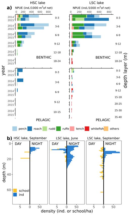
www.nature.com/scientificreports/
estimated the repeatability (R) index, both on data from the two lakes and on subsets of data for each lake, to
evaluate qualitative differences of repeatable patterns in temporal trend lines. Repeatability was calculated as:
Vtag_ID
,
Vtag_ID + Ve
where (Vtag_ID + Ve) is the total phenotypic variance ( Vp), resulting from adding the between-individuals vari-
ance (Vtag_ID) to the within-individual (residual) variance ( Ve). A high R may indicate high between- and/or low
within- individual variability in the outcome values (see SM1 for further details on repeatability index). As a
separate measure of repeatability, we compared the individual ranks in horizontal space use between June-July,
June–August, and June–September using the Spearman rank correlation test70. The same procedure was done
for swimming activity.
Stable isotopes. We ran linear models to test if the trophic niche of pike was related to individuals’ behaviour
(open-water use as a proxy), structural habitat complexity (SHC; lake factor as a proxy) or body length (i.e., total
length). Prior to modelling, open-water use was logit-transformed and continuous explanatory variables were
scaled (see above).
Growth. We used linear regression to find differences in individual growth (hypothesis v) in the previous sea-
son (log-transform of body increment in year 2014; dependent variable) between lakes and whether they were
determined by the space use (mean daily dH-KUD and dV-KS), body length and age of fish (explanatory vari-
ables).
Ethics approval and consent to participate. This study complied with and was approved by the Ani-
mal Welfare Committee of the Biology Centre CAS (45/2014) according to § 16a of the Act No. 246/1992 Coll.,
on the protection of animals against cruelty, as amended. The study was carried out in compliance with the
ARRIVE guidelines.
Consent for publication. This manuscript presents work that has not been published and is not under
consideration for publication elsewhere. All authors involved in the manuscript have agreed to be listed and
contributed to the research reported.
Results
Seasonal development of lakes environment. Both lakes were thermally stratified with the thermo-
cline gradually declining from 6–7 to 9–10 m during the study period (Fig. 2a,b). Oxygen concentration declined
below the thermocline during the season in the HSC lake, to such an extent that the water was anoxic from
14 m depth and deeper in September (Fig. 2a), whereas oxygen concentrations were similar (around 10 mg/L)
throughout the water column in the LSC lake at end of September (Fig. 2b). As expected the mean Structural
Complexity Index was significantly higher in the HSC lake than in the LSC lake (P < 0.001; tested using permuta-
tion inference, SM1 sec. Testing of Structural Complexity Index differences between lakes), but this difference
became much less in September as the Structural Complexity Index was relatively unchanged in the HSC lake,
but greatly increased in the LSC lake (P < 0.001 for the lake by macrophyte period interaction; Fig. 2c,d and areal
distributions of SCI is given in SM Fig. S7).
Gillnet fish densities in terms of both number and biomass were higher in the benthic habitats than in the
pelagic habitats in both lakes (Fig. 3a). In benthic habitats, gillnet fish densities and species composition were
similar in both lakes, following the same vertical pattern with a steep decrease with depth and low density of fish
below 12 m (Fig. 3a). Overall pelagic gillnet fish densities were slightly higher in the LSC lake, with whitefish
present in low numbers even in the largest sampled depth layers (30–35 m). Whitefish were not detected in the
HSC lake and almost exclusively only roach was captured in the pelagic zone in depths down to 9 m (Fig. 3a).
Hydroacoustic data showed almost no fish (school or single) in the HSC lake in September during the daytime
and only low abundance of fish at night (Fig. 3b). In the LSC lake, low densities of both schools and single fish
were detected in open water during the daytime in June and September and the number of single fish consider-
ably increased at night in the habitat during both months sampled (Fig. 3b).
Horizontal and vertical space use. The final models for horizontal and vertical utilization distributions,
daily mean depth and horizontal and vertical activity are summarized in Table 3. Model selection tables are
shown in Tables A2–A6 (Supplementary material).
The extent of explored horizontal area (dH-KUD) was significantly higher in the LSC lake (t = − 3.311,
P < 0.01), with temporal trends being positive and marginally varying between lakes (time × lake, t = − 1.94,
P = 0.052, SM1 sec. Extended results). dH-KUD significantly increased with body length in both lakes (t = 3.63,
P < 0.01) but with a steeper slope in the LSC lake (Least-squares means on body lengthslope ± SE, HSC lake:
0.14 ± 0.04; LSC lake: 0.37 ± 0.05; t = − 3.552, P < 0.01) (Fig. 4a). Water temperature was negatively related to
horizontal range (t = − 2.42, P < 0.05, SM1 sec. Extended results). Repeatability in the LSC lake was more than
1.6 times the amount observed in the HSC lake (R ~ 0.49 vs. 0.31) clearly showing more intra-individual varia-
tion under low structural complexity (Fig. 4b). These results are consistent with the Spearman rank correlation
tests by time periods, for June-July (Spearman’s Rho; LSC lake: ρ = 0.93; HSC lake: ρ = 0.46), June–August (LSC
lake: ρ = 0.75; HSC lake: ρ = 0.20), and June–September (LSC lake: ρ = 0.78; HSC lake: ρ = 0.20). The higher coef-
ficients in the LSC lake were associated with greater inter-individual variation in respect to dH-KUD (Fig. 4b).
Scientific Reports | (2021) 11:17472 | https://doi.org/10.1038/s41598-021-96908-1 7
Vol.:(0123456789)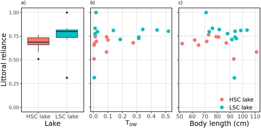
www.nature.com/scientificreports/
Figure 2. Temperature and oxygen stratification of water column at HSC (a) and LSC lakes (b), (c) distribution
of SCI in SCI-rasters covering 0–15 m depth (SCI) in both lakes and (d) vertical distribution of the Structural
Complexity Index (SCI) in both lakes. In (c) each point represents SCI value for 1 m2 of bottom. The bar in
the middle of the box shows the median, lower and upper hinges of the box correspond to the 25th and 75th
percentiles. The lower and upper whisker extends from the hinges to the smallest and largest value, respectively,
no further than 1.5 * IQR from the hinge (where IQR is the inter-quartile range, i.e. the distance between the
25th and 75th percentiles). Note the logarithmic scale of the y-axis. In (d) lines show mean SCI on depth profile,
given separately for each macrophyte sampling session.
In general, vertical utilization distribution (dV-KS) was not significantly different between the lakes (t = 1.68,
P = 0.11), and likewise with temporal trends (time × lake, t = 0.99, P = 0.322). It increased as the water tempera-
ture decreased irrespective of the lake’s structural complexity (t = − 2.88, P = 0.004, SM1 sec. Extended results).
Variability in vertical range use over time was marked between lakes, with pike in the HSC lake showing less
inter-individual variation than conspecifics in the LSC lake (R ~ 0.18 vs. 0.15) (Fig. 5).
Mean daily depth of pike in general increased with time (t = 2.74, P = 0.006) but it was not significantly differ-
ent between lakes (t = − 1.07, P = 0.29) and likewise across-lake temporal trends (time × lake, t = − 0.83, P = 0.41)
(Fig. 6) It showed a positive relationship with body length (t = 2.62, P = 0.016) and water temperature (t = 2.15,
P = 0.031, SM1 sec. Extended results). Inter-individual variation in mean depth across time was very similar in
the two lakes (R ~ 0.40) (Fig. 6c,f) and differences were mostly due to varying distribution patterns in the water
column (Fig. 6a–e). In the benthic habitats, pike were dispersed from the surface down to 12–15 m in the HSC
lake throughout the season, while in the LSC lake pike utilized even deeper depths down to 35 m at the end of
the summer (likely even deeper but the depth sensor could not record depths below 35 m). In open water, pike
were distributed primarily around the thermocline (Fig. 6).
Activity. Regardless of when it was measured, pike from the LSC lake were generally more horizontally active
than those from the HSC lake (t = 4.03, P < 0.001) with temporal trends in opposite directions, decreasing in
the LSC lake and increasing in the HSC lake (time × lake, t = − 2.48, P = 0.013) (Fig. 7a). Irrespective of the lake
complexity, body length was positively associated with fish activity (t = 2.34, P = 0.028) while water temperature
adversely influenced this behaviour parameter (t = − 3.38, P < 0.001, SM1 sec. Extended results). Repeatability in
swimming activity was generally higher in the LSC lake than in the HSC lake (R ~ 0.30 vs. 0.36), consistent with
Scientific Reports | (2021) 11:17472 | https://doi.org/10.1038/s41598-021-96908-1 8
Vol:.(1234567890)www.nature.com/scientificreports/
Figure 3. (a) Gillnet abundance of fish stock in both lakes, given separately for each sampled depth layer and
separately for bentic and pelagic habitats in one year prior to study (2014) and during study period (2015). (b)
vertical distribution of open water hydroacoustic densities separately in both lakes and diel periods.
the Spearman rank correlation tests for June-July (LSC lake: ρ = 0.68; HSC lake: ρ = 0.45), June–August (LSC
lake: ρ = 0.73; HSC lake: ρ = 0.05), and June–September (LSC lake: ρ = 0.50; HSC lake: ρ = 0.11). These results
Scientific Reports | (2021) 11:17472 | https://doi.org/10.1038/s41598-021-96908-1 9
Vol.:(0123456789)www.nature.com/scientificreports/
Horizontal activity
dH-KUD log(ha) dV-KS log(m) sqrt(m/s) Vertical activity sqrt(m/s) Depth log(m)
(Intercept) 0.77*** [0.625–0.92] 1.54*** [1.27–1.80] 0.045*** [0.035–0.06] 0.005*** [0.004–0.006] 1.47*** [1.20–1.75]
Time × lake − 0.003* [− 0.005–2 × 10–05] 0.002 [− 0.002–0.005] − 2.00** [− 4.00–0.40] × 10–04 1.00 [− 1.00–3.00] × 10–05 0.002 [− 0.002–0.006]
–04
Time 0.002* [− 3 × 10 –0.004] − 0.001 [− 0.003–0.002] 0.30 [− 1.00–1.00] × 10–04 0.00 [− 1.00–1.00] × 10–05 0.004*** [0.001–0.007]
Lake 0.39*** [0.18–0.60 0.11 [− 0.08–0.30] 0.03*** [0.02–0.05] 0.001 [− 0.001–0.002] − 0.21 [− 0.60–0.18]
Body length × lake 0.24*** [0.11–0.37]
Body length 0.14*** [0.06–0.21] 0.006** [0.001–0.01] 0.19** [0.05–0.34]
Water temperature × body
0.02* [− 0.002–0.04]
length
− 2.00*** [− 3.00–
Water temperature − 0.03** [− 0.05–0.005] − 0.02*** [− 0.03–0.005] − 0.003*** [− 0.004–0.001] 0.05** [0.004–0.10]
1.00] × 10–04
Random effects
σ2e 0.08† [0.070–0.085] 0.18† [0.17–0.20] 3.81† [3.45–4.21] × 10–04 3.66† [3.37–3.97] × 10–06 0.27† [0.24–0.31]
–04 –06
τ00 tag_id 0.06*** [0.028–0.122] 0.04*** [0.014–0.12] 2.84*** [1.36–5.95] × 10 1.51*** [0.59–3.83] × 10 0.18*** [0.08–0.43]
τ11 time 1.02*** [0.50–2.08] × 10–05 1.64*** [0.76–3.53] × 10–05 3.56*** [1.63–7.80] × 10–08 4.04*** [1.88–8.65] × 10–10 1.96*** [0.72–5.34] × 10–05
ρ01 tag_id.time − 0.82*** [− 0.93–0.58] − 0.75*** [− 0.91–0.37] − 0.73*** [− 0.89–0.38] − 0.60** [− 0.84–0.14] − 0.64** [− 0.87–0.16]
ρ AR(1) 0.72*** [0.65–0.77] 0.59*** [0.46–0.69] 0.73*** [0.66–0.79] 0.54*** [0.42–0.64] 0.78*** [0.72–0.82]
ρ MA(1) − 0.26*** [− 0.34–0.18] − 0.21*** [− 0.35–0.07] − 0.24*** [− 0.33–0.15] − 0.11*** [− 0.25–0.03] − 0.12*** [− 0.21–0.04]
R 0.43 0.19 0.43 0.29 0.40
RLSC | RHSC 0.49 | 0.31 0.15 | 0.18 0.36 | 0.30 7.25 × 10–05 | 0.51 0.40 | 0.41
R2m/R2c 0.43/0.60 0.07/0.29 0.23/0.47 0.08/0.40 0.15/0.43
Table 3. Final linear mixed-effects models analysing pike behavioural traits in low (LSC) and high (HSC)
structurally complex lakes. The variables analysed were both horizontal (dH-KUD) and vertical (dV-KS)
utilization distributions, horizontal and vertical activity, and mean daily depth. All variables were modelled by
fitting an ARMA autocorrelation structure of order (p = 1, q = 1). Data show β standardized estimates (mean-
centred and scaled by 2 s.d.) and 95% confidence intervals; the response variable remains untransformed. LSC
lake was set as the reference level. Random effects: σ2e, residual (within-individual) error variance; τ00 tag_id,
random intercept variance (i.e., variation between individual intercepts and average intercept); τ11 tag_id.time,
random slope variance (i.e., variation in individual temporal slopes across days); ρ01 tag_id, random slope-
intercept correlation (i.e., correlation between the individual random intercepts and slopes); R, adjusted
repeatability computed from fitted LMMs measuring the proportion of intra and/or inter- individual variation
over time; R SHC, R LSC, adjusted repeatability computed for each lake dataset separately (see main text for more
details). Significance values of random-effects parameters were computed using likelihood ratio tests between
each two nested models varying only in their random-effects structure (only p-value of the χ2 test is shown).
ρ AR(1), parameter Φ of the autoregressive correlation term AR(1); ρ MA(1) parameter Θ of the moving average
correlation term MA(1). R2m, marginal r-squared reflecting the proportion of variation explained by fixed
effects; R2c, conditional r-squared indicating the proportion of the variance explained by fixed and random
effects. Significance values for the regression estimates: *p < 0.1; **p < 0.05; ***p < 0.01. † No p-value was
computed.
indeed reveal higher levels of intra-individual variation under low structural complexity in the HSC lake show-
ing significantly less inter-individual variation (Fig. 7b).
In principle, vertical activity was not significantly different between lakes (t = 0.99, P = 0.33) nor was their
temporal trends (time × lake, t = 1.15, P = 0.25). However, we observed that either by ignoring or dropping the
time by lake interaction from the model, differences become significant (both: Least-squares means on lake ± SE,
HSC lake: 5.2 × 10–03 ± 3.2 × 10–04; LSC lake: 6.1 × 10–03 ± 3.1 × 10–04; t ~ − 2, P < 0.05), suggesting that swimming
speeds were on average different in both lakes at the end of the study (Fig. 7c). This also implies that regardless
of the measurement time, the LSC lake’s mean vertical activity is always higher than the HSC lake’s. In turn,
increased vertical activity was generally associated with decreased water temperature (t = − 3.14, P = 0.002, SM1
sec. Extended results) but this effect disappeared after including this variable in an interaction with factor lake
making between the lakes variation significant (lake, t = 2.35, P = 0.028). Consequently, despite the downward
trend in swimming speeds with temperature in the LSC lake, means in this lake kept generally above HSC
lake. Yet, even if the temperature by lake interaction was preferred (model 3 vs. model 4, Likelihood-ratio test,
χ211,12 = 13.47, P < 0.001; Table A6, Supplementary material), the temporal effect, while not mutually exclu-
sive, appeared to be a more satisfactory explanation to the observed differences between lakes based on AIC.
Inter-individual variation in vertical space use was significantly greater in the LSC lake than in the HSC lake
(R ~ 7.25 × 10–05 vs. 0.51), consistent with the observed patterns of variability over time (Fig. 7d).
Pelagic habitat use and food resources. The analysis of time spent in open water (TOW) is shown in
Table 4 with model selection in Table A7 (Supplementary material). TOW differed between lakes and as a non-
linear function of both dH-KUD and dV-KS (Fig. S8, Supplementary material). Overall, TOW (lake(μ), t = 7.99,
P < 0.001) was higher and more variable (lake(σ), t = 7.70, P < 0.001) in the LSC lake and increased over time
Scientific Reports | (2021) 11:17472 | https://doi.org/10.1038/s41598-021-96908-1 10
Vol:.(1234567890)www.nature.com/scientificreports/
Figure 4. (a) Dependence of daily extent of horizontal area (dH-KUD) and body length of observed pike, (b)
dH-KUD of each individual in each month. Dots represent mean values for the whole observed season/month,
error bars denote standard deviation. Colours in (b) were set according to body length of tracked individuals.
(time(σ), t = 4.05, P < 0.001, Fig. 8a). Higher levels of dH-KUD were correlated with increased likelihood of TOW
in both lakes (dH-KUD(μ), t = 7.99, P < 0.001, Fig. 8b), while increasing dV-KS was associated with a decreased
likelihood (dV-KS(μ), t = − 9.54, P < 0.001, Fig. 8c) but increased variability (dV-KS(σ), t = − 5.30, P < 0.001), with
both effects persisting over time. Only factor lake was significantly associated with each of the ν and τ compo-
nents representing probability of exclusive use of benthic habitats (p(TOW) = p0) or exclusive use of pelagic
habitat (p(TOW) = p1) respectively. Holding other covariates at fixed values, fish in the LSC lake were less likely
to use the benthic habitat only (p(TOW) = p0) than fish in the HSC lake (OR 0.721 [0.55–0.95], P = 0.02), which
was associated with higher dH-KUD (OR 0.21 [0.17, 0.25], P < 0.001) and body length (OR 0.841 [0.73, 0.96],
P = 0.012). Also, fish in the LSC lake were more likely to use the pelagic habitat only (p(TOW) = p1) than fish in
the HSC lake (OR 16.35[1.83, 146.33], P = 0.0125) irrespective of dH-KUD and body length.
A significant effect of lake and a negative effect of body length were found on pike littoral reliance (Fig. 9,
Tables 5, 6). The second best equally supported model (ΔAIC = 1.42) also suggested a positive effect of open
water use on littoral reliance (Table 5). In both lakes, pike seemed to shift to a less littoral (i.e., more pelagic) diet
with increasing body length (Fig. 9). Unexpectedly, pike tended to rely more on littoral resources in the LSC lake
(Fig. 9), where the individual with the lowest littoral reliance estimate (excluded from modelling) also showed
the lowest use of open-water areas. In fact, the stable isotope data indicates that only this single pike relied more
on pelagic than on littoral food resources (further results of SIA analysis are given in SM1, sec. Extended results).
Growth. The final and alternative models of pike growth are shown in Table A8 (Supplementary material).
Growth varied between lakes (Least-squares means ± SE, HSC lake: 90 ± 16.5; LSC lake: 142 ± 13.5; t = − 2.157,
Scientific Reports | (2021) 11:17472 | https://doi.org/10.1038/s41598-021-96908-1 11
Vol.:(0123456789)www.nature.com/scientificreports/
Figure 5. Daily extent of vertical space use for each individual in each month. Dots represent mean values for
the whole observed month and error bars denote standard deviation. Colours are set according to body length
of tracked individuals.
Figure 6. Two-dimensional distribution of all pike positions (dots) in relation to bottom depth for HSC lake
(a, b) and LSC lake (d, e) and depth use for each individual in each month (c, f). Isoclines depict the highest
concentration of positions in the benthic (orange) and open water (light blue) habitats. Mean thermocline depth
within each period is indicated by a dashed line.
Scientific Reports | (2021) 11:17472 | https://doi.org/10.1038/s41598-021-96908-1 12
Vol:.(1234567890)www.nature.com/scientificreports/
Figure 7. Development of mean horizontal and vertical activity during tracking period. Pooled (a) and
individual (b) horizontal activity; pooled (c) and individual (d) vertical activity in each month of tracking.
Dots represent mean values for the whole observed season/month and error bars indicate standard deviations.
Colours in (b) and (d) were set according to body length of tracked individuals.
P = 0.045), and with the age of individuals (t = − 3.90, P < 0.01), while no significant correlation was found
with body length. Given a significant crossover interaction between dH-KUD and dV-KS (dH-KUD × dV-KS,
t = 2.448, P = 0.025), we ran an interaction analysis to further determine the nature of the relationship between
those variables and growth rate. The result showed a conditional effect of dH-KUD on growth as a function of
dV-KS with growth increasing as dH-KUD increases at higher dV-KS values and decreasing with dH-KUD at
lower dV-KS values (see SM1 for further details, sec. Analysis of growth rate using linear regression).
Discussion
Structural complexity was found to have a strong directional influence on multiple pike behavioural traits, with
clear differences between the LSC and the HSC lakes. As hypothesized, pike exhibited higher horizontal space
use and higher activity in the LSC lake as compared to the HSC lake. Moreover, the increased space use with
increased activity also indicates that higher activity levels were associated with exploring new areas rather than
revisiting already visited areas. Exploration of more extended areas was positively related to pike size and linked
with higher use of open water, also reflected in lower littoral reliance in the diet. There was a high degree of
consistency in individual behaviour, individuals having high space use, activity and/or open water use in one
month, also had so in the next month (high repeatability) when there was a high degree of between-individual
variation. Inter-individual differences varied between lakes, with activity and exploration of horizontal space
showing higher individual rank correlation between months in the LSC lake where the between-individual vari-
ation was high. With low-between-individual variability, rank correlation between months also tended to be low.
Although rank correlation decreased over time in both lakes, the correlation was consistently much higher in
the LSC lake. Contrary to what was expected, individual growth was overall higher in the LSC lake, indicating
that pike in the LSC lake were able to more than compensate for increased activity costs by increased foraging
success. Despite observed differences in pike behaviour and growth, stable isotopes showed a low degree of
specialization and a high dependence on littoral food sources in both lakes.
Horizontal space use and activity. We found that activity and horizontal space use and activity were
higher with lower structural complexity. Predator space use is largely driven by prey abundance and predator
body size71–73, and a positive relationship between pike body size and horizontal space use has been previously
documented in numerous studies23,31,74–77. Previous research on predators capable of performing both active
pursuit and ambush strategies indicated that a switch between these modes was primarily linked to prey density
or prey type78–81. However, contrary to general expectations, prey abundance alone cannot explain the larger
Scientific Reports | (2021) 11:17472 | https://doi.org/10.1038/s41598-021-96908-1 13
Vol.:(0123456789)You can also read