COVID-19 and Strategic Sectors in Brazil: A Socially-Embedded Intersectional Capabilities Approach - Munich Personal ...

Munich Personal RePEc Archive

COVID-19 and Strategic Sectors in
Brazil: A Socially-Embedded
Intersectional Capabilities Approach

Haider, Khan and Szymanski-Burgos, Adam

Josef Korbel School for International Studies, University of Denver

August 2021

Online at https://mpra.ub.uni-muenchen.de/109022/
MPRA Paper No. 109022, posted 24 Aug 2021 05:51 UTC

COVID-19 and Strategic Sectors in Brazil: A Socially-Embedded
Intersectional Capabilities Approach

Haider A. Khan and Adam Szymanski-Burgos

University of Denver

Author Details

Haider A. Khan is a John Evans Distinguished University Professor, Policy Research Institute
Distinguished International Advisor, European Economic and Social Committee Former Senior
Scholar and Senior Research Fellow, Asian Development Bank Institute, Tokyo, Japan; and a
Professor of Economics at the University of Denver Josef Korbel School of International Studies.
He is on the board of editors and advisor to several economics and social science journals.
Correspondence concerning this article should be addressed to Haider A. Khan, Phone Number:
720-748-2555. Email: Haider.Khan@du.edu

Adam Szymanski-Burgos holds an MA degree from the University of Denver, Department of
Economics and is a research assistant for the Frederick S. Pardee Center for International
Futures. Email: szymanskiburgos@gmail.com

 1

Abstract

COVID-19 impacts have exacerbated socioeconomic inequalities and the threat of hunger and
absolute poverty for vulnerable populations globally. Brazil, as a large Southern engine of growth,
is a complex case. In responding to the public health impacts and economic challenges of the
pandemic, the case of Brazil stands out for several reasons. First, what was distinctive about
Brazilian public health policy and what have been the consequences so far? Second, what
circumstances and economic policy measures have led to a V-shaped recovery? Finally, what is
the further prognosis for Brazil over the next few years and what are the points of leverage to
ensure a sustained recovery? Our analysis highlights the salience of considering development and
the economic and social shocks of pandemics from a Socially Embedded Intersectional Approach
(SEICA) perspective. Using an economy-wide modelling methodology, we identify ‘strategic’
sectors in the Brazilian economy defined as sectors critical for both pulling the wider economy out
of a recession and for supporting widespread income growth, particularly for those in the bottom
40% of households. Additionally, we are able to draw some conclusions that may be relevant for
the case of other economies in various stages of development, particularly those with sharply
uneven development patterns and large rural populations.

 2

1. Introduction
The social and economic impacts of COVID-19 present lasting policy challenges for
governments around the world. These economic impacts have exacerbated socioeconomic
inequalities and the threat of hunger and absolute poverty for vulnerable populations. Localized
outbreaks of COVID-19 in Latin America first identified in March 2020 were met with a
diversity of containment measures across the continent. However, country differences in public
health capabilities and lockdown severity meant that the spread of infection could not be rapidly
contained. In addition, new COVID-19 variants with higher potential for spread had emerged in
Brazil overloading the public health systems of the country and its regional neighbors.

By June 2020, Latin America had become the new epicenter for the pandemic, accounting for
more than a third of new COVID-19 cases globally (Etienne 2020). The majority of new
infections in Latin America remain concentrated in Brazil which, until recently, has had the
second highest number of COVID-19 cases globally. 1 As of July 2021, the number of confirmed
cases in Brazil totaled higher than 19 million people, far above Argentina (4.1 million),
Colombia (3.6 million), Mexico (2.4 million), Peru (1.9 million), and Chile (1.45 million). The
combined economic impact of lockdowns, consumption shocks, and the collapse of international
trade have resulted in an estimated 8.1 percent decline in regional GDP for Latin America, far
above the estimated 4.4 percent decline of global GDP (Cottani 2020)

Aside from exposure to the more infectious delta variant of COVID-19, the ongoing severity of
the pandemic across the continent is due to a number of important reasons. Generally speaking,
Latin American countries tend to suffer from fiscal burdens and high levels of informality
leading to weakness in public health capabilities. For instance, countries like Argentina and Peru
have tended to suffer higher rates of infection than Chile and Uruguay. In addition, significant
responsibility for the crisis at the level of individual countries falls on the impact of government
mishandling during critical periods. This is true in Brazil, which has one of the strongest
healthcare systems in Latin America (World Bank 2020). Despite this, the initial containment
response led by the Brazilian president has been characterized as an “underestimation” (Marson
and Ortega 2020) of the public health threat leading to a policy that was “loose, inarticulate, and
insufficient” (Pires et al. 2020).

Matters are made worse by the fact that Brazil’s public health capabilities are distributed highly
unevenly across the country, leaving poorer regions more vulnerable to the spread of infections,
particularly in the North and Northeast (World Bank 2020a). This highlights an additional risk
factor for pandemic severity in the high levels of inequality that persist in Latin America
between racial groups, regions, and social classes. The interaction between socio-economic
inequality and the spread of infections operate in a vicious cycle. On one hand, the spread of
infections is aggravated by structural inequalities. Low-income communities find themselves
more exposed to infection due to employment patterns that are more intensive in face-to-face
activities and because of low capacity for social distancing and sanitation in smaller houses and

1
 Brazil has had the second-highest number of cases from May 2020 until April 2021 when it was surpassed by
India.

 3

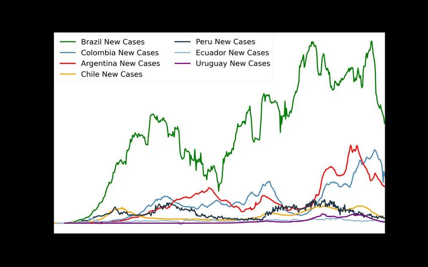
crowded neighborhoods. Minorities and other socially disadvantaged groups including black and
indigenous communities are uniquely susceptible to these issues due to the impacts of structural
racism, leading to their overrepresentation in essential face-to-face-intensive jobs and spatial
concentration in poorer areas. Lacking sustained access to quality healthcare and suffering in
higher likelihood of comorbidities, the poor are overall more likely to experience worse health
outcomes, including hospitalization and death (Pires et al. 2020).

On the other hand, the economic and social impacts of the pandemic are known to make income
and racial inequalities worse. Not only in Latin America but around the world, the loss of
incomes during the pandemic-driven recession appears to disproportionately affect workers in
the informal sector, lower-skilled workers, workers in services, retail, and construction, and the
self-employed (Pires et al. 2020). The disproportionate impact on the poor has directly led to an
increase in extreme poverty and hunger for hundreds of millions of Latin America’s poor and
vulnerable populations (ECLAC 2021). Moreover, the economic impacts of COVID-19 are made
worse given the ongoing developmental challenges in Brazil: stagnant productivity growth and
dependence on foreign investment.

Using Brazil as case study, we take a ‘key sectors’ approach to support a framework for sustainable
and inclusive recovery. We apply standard methods to rank economic sectors based on their
“power of pull” (PoP), defined as a sector’s capacity to influence other sectors through inter-
industry linkages and their degree of network centrality (Luo 2013). Using standard weighted
indicators for backward linkages and PoP we can produce a ranking of key sectors in Brazil based
on the extent of their backward linkages and their degree of connectedness. These describe the
extent to which economic influences are transmitted sector-to-sector in the event of a stimulus. In
addition to interindustry linkages and sector-level stimulus it is also important that policy
considerations in Latin America be examined through an intersectional lens with an emphasis on
targeted poverty reduction and the alleviation of structural inequalities as a means of achieving
longer-term recovery. Our framework is framed at the outset by a socially-embedded intersectional
capabilities approach (SEICA) (Khan 1998). This approach views development as a democratic
process where important feedback loops link macro-level outcomes with the material well-being
of disadvantaged and minority groups. Accordingly, the practical importance of a sector is the
direct or indirect impacts that is has on household income and consumption. We focus additionally
on the role of consumption linkages by estimating income, employment, and Type 2 output
multipliers.

2. Case Study: Brazil
After initial government attempts to flatten the curve failed, Brazil has suffered from relatively
high infection rates since May 2020 that have not shown any indications of slowing. The time
series in Figure 1.1 shows the comparative rate of infections in Latin America, with the 7-day
rolling average of new infections in Brazil greatly outpacing other major countries in the region.
The country has so far accumulated the highest level of infections and confirmed COVID-19
deaths in Latin America with upwards of 19 million accumulated cases and 540 thousand dead.
The continuing high rate of spread in Brazil has been linked to resurgent waves of infections in
neighboring countries (Schnirring 2021). Table 1.1 shows that, although Brazil leads all other
countries in terms of country-wide rates of infections and deaths, per capita rates have drifted
higher in countries like Uruguay and Argentina, which exceed Brazil in terms of average new

 4

cases per million and Peru, where the rate of new deaths per million far exceeds the rest of the
panel.

Figure 1.1 New COVID-19 Cases in Latin America, 7-day Rolling Averages

Source: Data sourced from Ritchie et al. (2020).

Table 1.1 COVID-19 Public Health Impacts in Latin America: May 2020 to July 2021
 Location Total Total Avg. New Avg. New Avg. New Avg. New
 Cases Deaths Cases Cases Deaths Deaths
 per Day per per Day per
 Million Million
 per Day per Day
 Argentina 4,769,142 101,955 9,481 209 204 4
 Brazil 19,391,845 542,756 38,202 179 1,108 5
 Chile 1,600,883 34,539 3,142 163 71 4
 Colombia 4,655,921 116,753 9,278 183 241 5
 Ecuador 476,312 21,958 946 53 45 2
 Peru 2,094,445 195,243 4,213 127 390 12
 Uruguay 379,072 5,889 774 221 12 3
Source: Data sourced from Ritchie et al. (2020).

Among the major differences in the observed rates of infections and deaths between Latin
American countries is the adequacy of public health capabilities and the effectiveness of
government response in terms of treatment and containment. Table 1.2 provides a comparative
snapshot of Latin American public health capabilities in response against COVID-19. Despite
having a strong overall healthcare system with significant coverage for public insurance, Brazil’s
capacity to provide quality healthcare is unevenly distributed throughout the country and health

 5

systems around the country quickly became overwhelmed with the growing number of
individuals needing medical care.

Table 1.2 Public Health Capabilities in Latin America: May 2020 to July 2021
 Location Avg. New Hospital Total Total People Avg. New Avg. New
 Tests per Beds Per Vaccinations Vaccinations Fully Vaccinations Vaccinations
 Day Thousand Per Hundred Vaccinated per Day per Million
 Per per Day
 Hundred
 Argentina 26,218 5.00 27,430,531 61 12 156,724 2,902
 Brazil 57,309 2.20 124,113,911 58 16 650,362 3,094
 Chile 38,840 2.11 24,761,379 130 61 120,785 6,258
 Colombia 51,711 1.71 23,631,963 46 20 141,547 2,980
 Ecuador 3,439 1.50 8,178,327 46 11 75,267 2,288
 Peru 10,226 1.60 10,781,431 33 12 67,384 1,950
 Uruguay 6,576 2.80 4,542,957 131 60 31,990 9,117
Source: Data sourced from Ritchie et al. (2020).

While Brazil had adequate supply of medical equipment (including hospital beds, ventilators,
and oxygen supplies) for the first wave of infections, these were not distributed equally across
regions. Most of the country’s intensive care units (ICUs) and hospital beds are located in urban
areas and state capitals, with the highest concentration of ICUs in three states: Sao Paulo, Rio de
Janeiro, and Minas Gerais (Marson and Ortega 2020). This has left rural groups and indigenous
populations at a structural disadvantage, facing additional barriers to access to quality healthcare
and disease prevention and sanitation equipment. Social and economic inequalities in general
have severely exacerbated the spread of infection and the rate of casualty. The bottom 40 percent
of households and the growing population of newly poor are highly disadvantaged by increased
susceptibility to infections. This is especially true for those living in urban favelas where basic
sanitation infrastructure is lacking and high population density makes social distancing
exceedingly difficult.

The total severity of the pandemic in Brazil has worsened the economic impacts on a country
already struggling to generate a meaningful recovery from the latest recession and political crisis
in 2015. This recession marked the end of a ‘golden decade’ of rapid growth and development in
Brazilian history. From around 2000 to 2015, Brazil saw a deep reduction in income inequality
and poverty driven by a boom in export commodities and positive labor market developments
enabled by fruitful policy shifts including the universalization of basic education in the 1990’s
and the elevation of the real minimum wage over time (Firpo and Pieri 2018). Poverty decreased
most rapidly in the North and Northeastern regions where poverty rates are the highest (this
remains true) and sustained declines in income inequality were driven by a narrowing of earnings
gaps between regions, gender, and race (Soares et al. 2016; World Bank 2020a).

The 2015 recession was caused in part by the ‘disarray of expectations’ that arose in light of a
series of policy shocks and scandals in 2015 (Arestis et al. 2021). A set of fiscal austerity
measures were introduced during the inauguration of Dilma Rouseff’s second term a bid to
reverse Brazil’s slowing economic growth performance of 2014 by reducing inflation and

 6

restoring investor confidence. Austerity measures included cuts to government expenditures for
social benefits, tax increases, reduction of subsidies, interest rate hikes, and the lifting of price
controls of public and administered prices. Negative shocks to GDP and employment (especially
concentrated in the MSE sector) resulted immediately from these measures. Despite these
measures, inflation continued to increase, and Brazil’s economic problems worsened as the
presiding administration entered a crisis of confidence leading into the Lava Jato corruption
scandals and Rouseff’s subsequent impeachment.

Authorities in Brazil have turned in favor of further austerity reforms to pursue fiscal
consolidation and achieve long-run growth under the guiding philosophy of “expansionary fiscal
austerity,” beginning with the highly controversial spending cap rule (Amendment 95) in 2016
under Michael Temer and more recently with 2019 pension reforms under Jair Bolsonaro. Under
Amendment 95, the primary annual expenditures of the federal budget have been restricted to
grow above an effective real rate of 0% over the term 2017-2037 as spending limits can only
adjust with the rate of inflation. The economic recovery has thus far depended on the ability of
federal and state governments to rebuild weakened fiscal buffers and restore market confidence.
By 2020, however, these reforms had not led to a significantly stronger fiscal situation for state
governments (World Bank 2020a). Rather, they have dramatically weakened the government’s
capacity to respond to the economic and health challenges of the pandemic (Arestis et al. 2021).

Figure 1.2 GDP Growth in Brazil: 2015-2021

Source: FRED

On top of this weakened fiscal and economic position, the recovery turned into a huge
contraction with the onset of the pandemic. The initial shock is reflected in a 33.5 percent drop in
GDP in the second quarter of 2020, an economic decline that was relatively mild compared to

 7

other countries in the region (Cottani 2021). A relatively strong V-shaped recovery began in the
third quarter of 2020, driven largely by a massive injection of government funds. In addition, the
aggregate shock has been buffered somewhat thanks to looser quarantine restrictions and the
recovery of export-oriented sectors, which have seen positive growth in 2020 due to adjustments
in the real exchange rate and the recovery of import orders from China, the country’s largest
export market. Overall, Brazil saw a total year-by-year decline of 4.1 percent of GDP in 2020,
beating some of more pessimistic forecasts from the World Bank and IMF (McGeever 2021).
Although the aggregate decline of the pandemic may have been lower than expected, there have
been lasting impacts concentrated in the service industries, particularly retail trade,
transportation, and accommodation.

Table 1.3 Brazil’s Top Export Partners
 Country Exports (in Imports
 billion (in billion
 USD) USD)

 China 63.4 35.3
 United 29.8 30.4
 States
 Netherlands 10.1 2.1
 Argentina 9.8 10.6
 Japan 5.4 4.1
Source: Figures for 2019 are sourced from World Integrated Trade Solutions

Table 1.4 Brazil’s Top 10 Export Commodities
 Country Exports (in Percentage
 billion of Total
 USD) Exports

 Soybeans 26.1 11.4%
 Crude 24.3 10.6%
 Petroleum
 Iron Ore 23.0 9.99%
 Corn 7.39 3.21%
 Sulfate 7.35 3.19%
 Chemical
 Woodpulp
 Poultry 6.55 2.85%
 Meat
 Refined 5.76 2.5%
 Petroleum
 Soybean 5.9 2.56%
 Meal
 Bovine 5.67 2.47%
 Meat
 Raw Sugar 5.33 2.32%
Source: Figures for 2019 are sourced from World Integrated Trade Solutions

The export ‘boost,’ which has contributed significantly to Brazil’s economic recovery path, is a
result of recovery in industrial production in other countries, particularly in China and other
major trading partners (see Table 1.3). However, despite its apparent usefulness for providing

 8

economic buffers from crises and stimulating short-term recovery, Brazil’s export model is
concentrated on low value-added commodities such as agricultural products and basic materials
including crude petroleum and iron as well as some semi-manufactured products (Table 1.4).
This model is arguably limited for creating further growth since it embodies the well-known
“middle-income trap” for many developing countries.

Figure 1.3 Unemployment Rate in Brazil: 1995-2021

Source: FRED

While unemployment rates remained relatively low from 2010 to 2014 hovering around 6-7
percent, the recession led to a sharp increase in unemployment upwards of 13 percent by around
2017 through 2020 shown in Figure 1.3. Increases in unemployment have been coupled with
falling real wages and depressed government expenditures under austerity, leading to a reduction
of past social welfare gains and the growing threat of poverty for millions of Brazilians. The
proportion of people in Brazil living in poverty or vulnerable to poverty is estimated at around
half of the total population. According to the World Bank’s Report (2020a), this section of the
population was especially vulnerable to the economic and social impacts of the pandemic since
there was virtually no recovery of incomes since 2016 for this level. Since the onset of the
pandemic, these groups have seen the largest relative declines in income. The increase in
unemployment has been concentrated in the bottom 40 percent of income earners. Both income
inequality and the rate of poverty have increased in 2020, with a total estimate of 7.2 million
additional Brazilians facing poverty.

The government has responded to the broader public health, economic, and social crisis with
significant policy measures and emergency fiscal spending. Using IMF (2021) data on cross-
country COVID-related expenditures, total fiscal expenditures in 2020 in Brazil (not including
direct public health expenditures) are estimated at a total of 848.6 billion BRL ($162.7 billion
USD), equivalent to 11.9 percent of GDP. Despite the federal spending cap still in place, Brazil’s
counter-COVID 19 expenditures are among the largest in Latin America both in gross terms and

 9

as a percentage of GDP.2 The government response is estimated to have limited the decline of
GDP in 2020 to 4.1 percent and generated an overall temporary drop in of 8 percent in the
national poverty rate in 2020 (World Bank 2021). The prevention and reduction of poverty
among vulnerable group is attributed directly to household transfer and assistance programs
through Auxilio Emergencial, the expansion of Bolsa Familia, and others.

Fiscal policy includes significant federal transfers to state governments experiencing budget
shortages and fiscal crises. Direct fiscal expenditures were directed toward two main ends: 1)
providing income supports and emergency aid for households and 2) channeling resources
toward aggregate employment stabilization using a range of direct supports and employment
incentives for small and micro enterprises (SMEs). Utilizing IMF (2021) data we can provide a
categorized breakdown of Brazil’s total package of counter-COVID 19 expenditures in 2020:
 • The implementation of an emergency income protection transfer program Auxilio
 Emergencial, which pays over half of a minimum wage for up to 3 months for uncovered
 workers that are unemployed mostly in the informal and self-employed sectors, accounts
 for roughly R$ 196 billion - 23.15% of total fiscal expenditures.
 • The expansion of Brazil’s Bolsa Familia federal conditional cash transfer program by an
 additional 1.2 million households accounts for an additional R$ 28.7 billion – 3.38 % of
 total fiscal expenditures
 • The implementation of the National Support Program for Micro and Small Enterprises
 (Pronampe) with several rounds of funding accounts for R$ 53.8 billion – 6.34% of total
 fiscal expenditures.
 • A large package of varied fiscal supports including tax cuts and employment incentives
 for small and medium enterprises (SMEs) through the Brazilian Development Bank
 (BNDES) and other agencies totaling $R 226.6 billion – 26.7% of total fiscal
 expenditures
 • A large package of other social assistance and emergency aid programs including
 unemployment insurance and food aid through a variety of agencies totaling $R 342.9
 billion – 40.4% of total fiscal expenditures

The monetary policy response was characterized by rate cuts from mid-February to August 2020,
to the historical low of 2 percent, and the introduction of a set of measures to increase liquidity in
the financial system. These included the reduction of reserve requirements from 25% to 17% and
a temporary relaxation of capital buffers and provisioning rules. Overall liquidity has also been
supported by Brazil’s special access to a dollar swap line with the US Federal Reserve, who has
established an available line of $60 billion USD for emergency use. According to the IMF (2021)
however, the majority of liquidity supports were withdrawn in 2021 including interest rates hikes
to 4.25% by June.

3. Methodology
The data for this analysis comes from the 2015 harmonized OECD IO tables. This dataset offers a
set of interindustry flows for 36 production activities for Brazil for all other OECD countries. Final

2
 According to our estimates using IMF (2021) data, Brazil had the largest sum of counter-COVID 19 fiscal
expenditures across the region. In terms of counter-COVID 19 expenditures as a percent of GDP, Brazil’s spending
package is second only to Chile, which spent or set aside an estimated 19% of GDP on total counter-COVID 19
fiscal expenditures in 2020.

 10

demand is divided into rural and urban household consumption, government consumption, gross
fixed capital formation (investment in fixed assets), changes in inventory, and exports. Total value-
added is then distributed among factors of production in the form of workers’ compensation, gross
operating surplus, production taxes, and capital depreciation.

3.1 Interindustry Linkages and Multiplier Analysis
The basis for investigating linkages and economic multipliers is the matrix of interindustry
transactions. This matrix offers a model of interindustry flows of products and resources within an
economy as well as resources flows to institutional accounts including households, taxes, capital
incomes, and exports. The interindustry transactions matrix describes the total output of each
production sector in the economy as it is distributed among purchasing sectors as intermediate
goods and among households and other agents as final goods. Data for interindustry flows are used
to construct the the matrix of direct sector requirements for the economy, describing the direct
sector requirements of production in terms of inputs of sector i for a unit of total output in sector
j.
Algebraically, this produces a system of equations with the general form (1) and matrix notation
(2):

 # = #& & + # (1)
 = + (2)

where #& is the technical coefficient representing the per-unit monetary value of input from sector
i required to produce a monetary unit value of output in sector j. In the matrix notation, x is a
column vector of total output produced by each production sector, y is a column vector of output
generated by final demand, and A is a square matrix of technical coefficients #& . A fundamental
assumption with the use of input-output tables is that, for a definite length of time, interindustry
resource flows from sector i to sector j depend entirely on the total output of sector j for the same
period of time. Conventionally in IO analysis, we assume this ratio is constant according to a fixed-
proportions production function with constant returns to scale.

If there is an increase in output from sector j then there will be an increase in intermediate demand
via sector j’s additional purchases from sectors which provide inputs to sector j. Similarly, if there
is an economy-wide increase in output for all sectors, then sector j can expect further increases in
output from additional purchases from all sectors that purchase inputs from sector j. These are
referred to as backward and forward linkages respectively and are considered to describe the
structural paths from which increases in output for one or a cluster of sectors are transmitted
throughout the wider economy in the form of interindustry flows.

If the vector of final demand y is known, the total output of each sector needed to supply both
intermediate and final demand requirements may be found as the solution to the following
equation:

 = ( − )./ (3)

where I denotes the identity matrix, and the inverse matrix ( − )./ gives the matrix of total
requirements coefficients (Fjeldsted 1980). The product of the total requirements matrix and the

 11

vector of final demand y give the necessary output required from each of the sectors to satisfy total
demand in the economy. The elements of the total requirements matrix describe the direct and
indirect sector output effects for a change in final demand.

If we assume this change in final demand occurs for a single sector, then we consider the indirect
effects on the rest of the economy to depend on a size effect and a network effect. The size effect
refers to the increased economic influence gained with economies of scale and is measured by the
relative size of the sector in terms of output or value-added. The network effect can be measured
in part by interindustry linkages between that sector and other sectors in addition to consumption
linkages between that sector and factor-supplying households.

One way to measure the network effect of a sector is to estimate its output multipliers. Summing
the elements of the ( − )./ matrix in column j gives the output multiplier for sector j, defined
as the amplified effect of an economic stimulus as money is spent and re-spent in an economy over
several rounds. Formally, the output multiplier is defined in Miller and Blair (2009) as the sum of
the column elements ( #& ) for sector j in the inverse matrix

 ( )& = ∑4#5/ #& (4)

For a given sector, the output multiplier measures the combined direct and indirect effect of a unit
change in sector output including the additional change in output of all industries in which that
sector purchases inputs. To produce an additional $100 worth of machine parts requires the
additional purchasing of local inputs (e.g. steel, electrical components, and transport services) as
well as the purchasing of local labor services. An output multiplier of 1.5 indicates that a direct
increase of $100 in final demand for machine parts can generate an additional increase of $50 in
intermediate demand through sector linkages, leading to a total of $150 in economy-wide gains.

Output multipliers are known to capture both direct and indirect linkages. However, there is a long-
standing debate in the literature as to the inclusion of “internal linkages” (i.e. on-diagonal elements
of A or ( − )./ ) when one is interested in estimating a sector’s true “backward dependence” or
it’s linkages to the rest of the economy (Miller and Blair 2009). Various normalization methods
have been proposed using pre-multiplication of the A matrix by a unitary vector that allow for a
ranking of sectors by the magnitude of backward and forward linkages. The three most wide-
ranging measures of linkages were developed by Chenery and Watanabe (1958), Rasmussen
(1957), and Dietzenbacher (1992). Borrowing notation from Morrone (2017), we can express
Chenery and Watanabe’s weighted direct backward linkage index as:

 = ne′A/e′Ae (5)

where n is the number of sectors in our model, e refers to a column summation vector (where ei=1
for all i), ′ denotes transposition, and A is the technical coefficient matrix. The sum of sector j’s
backward linkages is divided by the simple average of all backward linkages in the economy. The
average value of our index m is one so that sectors with an index value greater than one are
considered sectors with direct backward linkages that are above average. Similarly, sectors with a
value less than one are considered to have direct backward linkages that are below average.

 12

In the same fashion, Rasmussen (1957) used the inverse matrix to develop an index of normalized
total backward linkages that capture both direct and indirect output gains needed to match an
increase in final demand for sector j. We can express Rasmussen’s total backward linkage index
as:

 = ne′( − )./ /[e′( − )./ e] (6)

where ( − )./ is our inverse matrix.

The Dietzenbacher eigenvector method builds on the Chenery and Watanabe weighted direct
backward linkage index using an infinite iterative process where the vector m1 of linkage
indicators may be used as weights in place of the column summation vector e in a new calculation
of linkage indicators m2. In turn, the elements of m2 are used as weights for an additional
calculation in m3. In this fashion, the inputs from sectors with a higher power of pull are given
additional weighting than sectors with lower powers of pull. This iterative process takes the
following form:

 #>/ = n # ′A/ # ′Ae (7)

Thus, our estimation of sector power, as defined by backward linkages and a sector’s degree of
network centrality, is improved iteratively as i approaches infinity. Dietzenbacher (1992) proved
that the indicator #>/ converges to a function of the normalized left-hand eigenvector
corresponding to the dominant eigenvalue of the technical coefficient matrix A:

 #>/ = nq′/(q′e) with q′A = λA q′

where qB is the “Perron vector” i.e. the eigenvector corresponding to the dominant eigenvalue λA
of the matrix. The elements of the resulting vector nq′/(q′e) provide a robust measure of sectors’
power of pull considering both the weighting of backward linkages and the ‘infinite regress’ of
economic influences throughout a network or cluster of sectors (Luo 2003).3

Finally, we focus also on the demand-side role of consumption linkages in supporting a sustainable
and balanced recovery. An increase in the purchases of local labor inputs following an increase in
demand leads to higher household incomes and additional consumption expenditures. These
consumption linkages present an additional multiplier effect on the basis of induced increases in
output from increased household expenditures. By “closing” our IO model with respect to
households we can derive income and Type 2 output multipliers, which collectively describe the
total multiplier effects of direct, indirect, and induced increases in sector output. Closing our model
with respect to households refers to the inclusion of factor-supplying households as an endogenous
sector by including an additional row for labor compensation and an additional column for
household consumption in our intermediate matrix that we use to calculate our technical
coefficients table.

3
 In order for our model of the economy to be workable, the infinite series must be convergent since this is a
fundamental condition for there to be a solution.

 13

Identifying key sectors capable of supporting an inclusive and balanced recovery must involve
identifying those sectors with above-average consumption linkages, providing relatively large
flows of household income and employment. Income multipliers represent the economic impacts
of a change in final demand on household earnings and describe how the benefits to growth are
distributed to households. By considering household expenditures as endogenous, these multipliers
capture information regarding the magnitude of induced output effects which appear in our Type
2 output multipliers. Simple income multipliers are derived using the technical coefficients for
direct labor requirements when the IO model is closed with respect to households. The calculation
involves weighting each element in the direct labor requirements (households) row by the output
multipliers of the corresponding sector and taking the sum. This relation is described formally in
equation (8) where 4>/,# are the row elements of household income receipts from labor
compensation by sector.

 (ℎ)& = ∑4#5/ 4>/,# ( #& ) (8)

The simple income multiplier denotes the direct and indirect effect of an increase in final demand
for sector j on the total value of required labor services. There is another kind of income multiplier,
referred to as the Type 1 income multiplier, which describe how the initial sector-household
income payments 4>/,# are “blown up" over several rounds of direct and indirect spending effects
over the economy (Miller and Blair 2009). The formula for the Type 1 income multiplier is simply
the ratio of the simple income multiplier (8) and the labor input requirement coefficient 4>/,# .

 ∑G
 JMI FGHI,J (KJL )
 (ℎ)E& = (9)
 FGHI,J

While the simple income multiplier describes the increase of household incomes as a result of
additional labor input requirements for sector j, the Type 1 income multiplier captures the relative
contribution of income gains in sector j in stimulating additional income gains across sectors. Thus,
viewing the results of these income multipliers from a socioeconomic lens enables the
identification of critical sectors which can be leveraged to pursue strategic commitments for
sustained income growth and support of domestic markets. The major limitation of IO data in this
respect is the lack of delineation between various income or skill groups, accounts which
prominently feature in SAMs, to allow for identifying targeted income effects for low-income
households or low-skilled workers. Instead, we rely on external sources regarding the labor
intensity of the sector and the given sector’s demand for less-skilled labor.

Given that the household sector’s main “output” are labor inputs, our income multipliers are
closely related to a sector’s physical employment multipliers for a change in final demand.
 
Following (Kecek et al. 2021), we calculate ̂& = &Q P as the number of full-time employees in
 #
sector j where & is the total value of compensation paid to workers and #P denotes the monetary
value of sector output in the base year. The physical employment multiplier formally describes the
sector-to-household linkages through the labor market as the ratio of the initial increase of
employment a result of additional input requirements for sector j and the sector’s share of
compensation for full-time employment of output:

 14

∑G
 JMI R̂ J (KJL )
 ( )& = (10)
 R̂S L

This describes the number of additional direct and indirect gains in employment due to the
autonomous increase of one direct unit of employment in sector j. Although we cannot map sectoral
income effects to income or skill groups, if we know details about sector employment levels of
skill groups or average wages we can utilize the employment multiplier to identify sectors more
likely to impact lower-income households. Viewing the results of employment and income
multipliers from a socioeconomic lens enables the identification of critical sectors which can be
leveraged to pursue strategic commitments for sustained inclusive growth for those in poverty and
for disadvantaged groups. The major limitation of IO data in this respect is the lack of delineation
between various income or skill groups, accounts which prominently feature in SAMs.

4. Results and Interpretation
This section is structured as follows. First, we report our estimates for backward linkage indicators
and identify key sectors for the Brazilian economy. These linkage indicators serve as a proxy for
the power of pull of a given sector with respect to the rest of the economy and serve to clarify
which sectors should be bailed out first in the event of a recession (Morrone 2017). Sectors are
ranked according to their capacity to influence total economic recovery by virtue of direct
indicators (gross output, value-added, employment) and their interindustry linkages. We compare
rankings for sectors when all three indicators of backward linkages are considered. Following Luo
(2013), we provide a comparison of sectors’ power of pull using the eigenvector method with their
direct indicators. Second, we detail the results of our economic multiplier analysis for Brazil. We
describe our estimates for average multipliers. Then, we report a full set of multipliers for the
largest sectors by value-added in the overall economy, for pandemic-sensitive service industries,
the largest sectors in manufacturing, and in public health and social work. The significance of
sector multipliers is assessed within the context of the social and economic impacts of COVID-19
at the level of sectors and households.

4.1 Power of Pull Analysis
Generally speaking, the relative economic importance of a sector can be considered in terms of its
channels of influence structured by a particular size effect and network effect. Direct indicators
(intermediate consumption, output, value-added, and others) provide measurements of the size
effect while our backward linkage indicators provide measurements of the network effect.
Accordingly, each of these components of sector importance should be considered in light of the
others. In the context of planning for an economic recovery, it is more useful to focus on sectors’
network effects in order to leverage their ability to support and stimulate economic activity in other
sectors. We begin with Table 1.1 showing the top 10 sectors by Chenery and Watanabe (CW)
indicators and comparing them with the ranking for Rasmussen and Eigenvector-based PoP
indicators. Note that while our CW and Rasmussen indicators here are unweighted, the PoP
indicators are weighted iteratively for backward linkages and become highly sensitive to a sector’s
centrality in a cluster of sectors. Accordingly, eigenvalues have more to do with dynamics of the
system, denoting higher pull over time and the power to propel growth over the economy.

 15

Table 1.1 Comparing Interindustry Linkage Indicators
 Sector CW Rank Rasmussen Rank PoP Rank

 Coke and refined 1.621 1 1.429 1 3.597 3
 petroleum
 products

 Food products, 1.491 2 1.244 2 0.860 10
 beverages and
 tobacco

 Computer, 1.433 3 1.263 3 0.327 25
 electronic and
 optical products

 Manufacture of 1.421 4 1.246 4 0.768 11
 basic metals

 Motor vehicles, 1.417 5 1.289 5 0.355 23
 trailers and
 semi-trailers
 Other transport 1.378 6 1.252 6 0.115 32
 equipment

 Chemicals and 1.366 7 1.254 7 2.839 4
 pharmaceutical
 products

 Electrical 1.342 8 1.232 8 0.320 26
 equipment

 Rubber and 1.308 9 1.225 9 0.573 15
 plastics products

 Machinery and 1.229 10 1.135 10 0.512 17
 equipment

Source: Authors’ calculation

Comparing indicators across sectors, we find that the ranking of sectors by CW indicators share
the exact same ranking distribution as the Rasmussen indicators across all 36 sectors. This finding
suggests that the structure of direct and total backward linkages in Brazil are closely related and
confirms the well-known finding that CW indicators are highly correlated with Rasmussen
indicators (Morrone 2017). We find that coke and refined petroleum products stands above as the
sector with the largest values for both CW and Rasmussen indicators, followed by 2) food,
beverage, and tobacco products, 3) computer, electronic, and optical products, 4) manufacture of
basic metals, and 5) motor vehicles, trailers, and semi-trailers. These five sectors are distinguished
by higher than average levels of backward linkages. Thus, these sectors are considerably well-
positioned to support economic activity in connected sectors and drive overall economic growth
or recovery.

 16

Our results support the findings in Morrone (2017) which identified the relative importance of the
coke/refined petroleum, chemical/pharmaceutical products, basic metals, and food, beverages, and
tobacco products sectors. Although our finding of computer, electronic, and optical products (CW
rank #3) and motor vehicles (CW rank #5) as key sectors are at odds with Morrone’s estimated
rankings. Considering that the underlying data we work with corresponds with a later year and a
greater level of sector aggregation than in Morrone’s (2017) analysis using 2013 input-output data
with 51 production activities, we should expect some difference in our results, particularly due to
differences in the level of aggregation. However, it is within the realm of possibility that the
computer/electronics and automotive industries in Brazil have increased in importance in recent
years.

Comparing our CW and Rasmussen indicators with our eigenvalues, we find that these indicators
are very weakly correlated with eigenvalues (exhibiting Pearson coefficients of 0.007 and -0.015
respectively). Though our sector with the largest CW and Rasmussen indicators (coke and refined
petroleum products) indeed presents a relatively high PoP rank (3rd), we quickly find that the top
sectors by CW and Rasmussen indicators do not correspond generally with the top sectors by PoP.
Thus, at first comparison it appears that our indicators for sector importance by backward linkages
are dependent on different factors. It is clear that rankings between sectors by indicator tell a
different story than the CW and Rasmussen indicators by observing Table 1.2, which shows the
top 10 sectors by Eigenvector indicators. Notably, we find that the most important sectors by PoP
vary considerably from our previous method of ranking.

Table 1.2 Comparing Interindustry Linkage Indicators (Cont.)
 Sector PoP Rank CW Rank Rasmussen Rank

 Business sector 5.087 1 0.666 31 0.766 31
 services

 Wholesale and 5.023 2 0.696 28 0.780 28
 retail trade

 Coke and 3.597 3 1.621 1 1.429 1
 refined
 petroleum
 products

 Chemicals and 2.839 4 1.366 7 1.254 7
 pharmaceutical
 products

 Mining and 2.598 5 1.016 20 0.974 20
 extraction of
 energy
 products

 Transportation 2.103 6 0.983 23 1.005 23
 and storage

 17

Financial and 1.997 7 0.693 29 0.764 29
 insurance
 activities

 Electricity, gas, 1.782 8 1.070 16 1.025 16
 water supply,
 and other
 utilities
 Agriculture, 0.910 9 0.806 27 0.930 27
 forestry and
 fishing

 Food products, 0.860 10 1.491 2 1.244 2
 beverages and
 tobacco
Source: Authors’ calculation

Comparing our CW/Rasmussen measures of backward linkages and eigenvalues yields
fundamentally different results. The sectors with the largest eigenvalues generally correspond to
low CW/Rasmussen rankings, with the notable exception of coke and refined petroleum products
and chemical/pharmaceutical products, which do have relatively large CW/Rasmussen indicators.
The business sector services has a PoP rank of 1st but is 31st in both CW and Rasmussen indicators.
Similarly, wholesale and retail trade had a PoP rank of 2nd but is 28th in both CW and Rasmussen
indicators. This result is unusual compared to Dietzenbacher’s (1992) study of linkage indicators
in the Netherlands, finding a general cross-similarity in the ranking distribution of sectors by
alternative linkage indicators. This difference may be accounted for by key differences in the
production structure and concentration of linkages in developed and developing countries (Laumas
1975), particularly in developing countries’ greater dependence on fewer sectors.

We find that the sectors with the greatest PoP according to eigenvalues are 1) business sector
services, 2) wholesale and retail trade, 3) coke and refined petroleum products, 4) chemicals and
pharmaceuticals, and 5) mining and extraction of energy producing products. Of the top five
eigenvalues, only one corresponds with a top five sector by CW/Rasmussen indicator: coke and
refined petroleum products. Given that we find the coke and refined petroleum products and
chemical/pharmaceutical products sectors on the upper end of both rankings of both PoP and
CW/Rasmussen indicators they clearly represent strongly networked sectors upon which large
sections of the Brazilian economy depend on for intermediate demand. The Eigenvector method
accounts for the optimal weighting of sector linkages over infinite regress and is therefore sensitive
to clustered sectors. Patterns of sector-to-sector concentration in intermediate purchases and sales
tend to inflate eigenvalues for some sectors while reducing those for others (Dietzenbacher 1992).
This well-known fact implies that the main differences in the rankings of sectors among alternative
methods is related to the relative concentration of intermediate input purchases for backward
linkages and intermediate output sales for forward linkages.

Sector with the greatest PoP act as major nodes for the economy as they serve to connect industrial
clusters in a complex web of backward and forward linkages. These sectors are marked by their
degree of connectednesss in a network made up of nodes and paths. The wholesale and retail trade
sector acts as a clearinghouse of sorts for commodities in various stages of production, providing

 18

an outlet for commodities from intermediate producers to reach other firms (wholesale) or
households (retail). In the case of business services, we find significant concentrations in forward
linkages. The business services sector is a major sector providing critical inputs for a large variety
of sectors across the economy. The size and importance of the business services sector is held to
growth in importance with greater tertiarization of the economy on the basis of these linkages
(Russo and Chies 2017). A high degree of concentration in forward linkages is true for a majority
of sectors with large eigenvalues, denoting sensitivity to large network centrality effects.

4.2 Does Size Matter?
As shown in Luo (2013), the ranking of sectors by their Eigenvector-based PoP may differ
significantly from the ranking of sectors by direct measures of importance, such as total
intermediate input, total output, and value-added. We turn to the question of whether this is true
for the Brazilian economy. Table 2.1 provides a comparison of sector rankings by their eigenvalues
and direct indicators of importance.

Table 2.1 Comparing Direct Indicators with Sectors’ Power of Pull
 Sector PoP Rank Intermediate Rank Sector Output Rank Value-added Rank
 Inputs ($mn) ($mn) ($mn)

 Business sector 5.087 1 $ 71,446 7 $ 195,797 3 $ 124,351 4
 services

 Wholesale and 5.023 2 $ 126,676 2 $ 333,062 1 $ 206,386 1
 retail trade

 Coke and refined 3.597 3 $ 102,002 4 $ 112,966 10 $ 10,964 25
 petroleum
 products
 Chemicals and 2.839 4 $ 85,015 5 $ 109,321 11 $ 24,307 16
 pharmaceutical
 products
 Mining and 2.598 5 $ 27,346 19 $ 47,610 18 $ 20,263 17
 extraction of
 energy products
 Transportation 2.103 6 $ 84,754 6 $ 152,926 6 $ 68,172 10
 and storage
 Financial and 1.997 7 $ 65,940 9 $ 175,880 4 $ 109,941 5
 insurance
 activities

 Electricity, gas, 1.782 8 $ 60,840 12 $ 97,912 12 $ 37,072 12
 water supply, and
 other utilities

 Agriculture, 0.910 9 $ 68,028 8 $ 145,972 7 $ 77,944 8
 forestry and
 fishing
 Food products, 0.860 10 $ 158,907 1 $ 196,074 2 $ 37,167 11
 beverages and
 tobacco

 19

Source: Authors’ calculation

We find that sectors may be distinguished by PoP rankings that are higher than sector rankings by
direct measures. This is true for chemicals and pharmaceutical products, which is ranked 4th in
PoP, and 5th in terms of intermediate inputs, but only 11th in output, and 16th in value added.
Similarly, the mining and extraction of energy products is ranked 5th in PoP, but only 19th in inputs,
18th in output, and 17th in value-added. Thus, the chemical/pharmaceutical products and raw energy
products sectors are distinguished by the fact that they are not large but ‘powerful’ as in capable
of exerting significant economic influence across sectors (Luo 2013). We find sectors also that are
both large and powerful, as in the case of wholesale and retail trade which is ranked 2nd in PoP,
2nd in terms of intermediate inputs, 1st in output, and 1st in value added.

Additionally, there are sectors that are large but exhibit lower than average PoP. Such sectors may
account for relatively large resource flows in the economy but not contribute large network effects.
One such sector is the food, beverages, and tobacco products sector which is the 2nd largest sector
in terms of output, the largest in terms of intermediate inputs and 11th in terms of value-added,
however it has a PoP ranking of 10th. Overall, we find that ranking sectors by their eigenvalues
yields results that are fundamentally different than when ranking sectors by their direct indicators.
The distribution of different rankings across our sectors enables us to distinguish between sectors
that are important because they are large and sectors that are important because they have a high
PoP and identifying sectors which may be both large and powerful as well as sectors which are
none. Assessing the relative importance of both direct measures (size effects) and measures of
backward linkages (network effects) in addition to the scope of their interactions are important for
developing sector-led recovery plans that are country-specific.

4.3 Multiplier Analysis
The PoP measure and the key sectors analysis in general in based on a gross output approach,
meaning that the magnitude of backward linkages can tell us relatively little about direct welfare
implications through income and employment effects. ‘Bailing out’ sectors with high
CW/Rasmussen and/or PoP indicators through exogenous increases in final consumption (i.e.
foreign investment, government spending) may result in temporary growth of income and
employment, however they cannot contribute directly (via demand-side channels) to welfare
implications through structural changes in the distribution of incomes or the structure of
employment (Luo 2013).

The significance of large output multipliers is similarly limited given that a large multiplier is
simply due to having large input coefficients. While these coefficients point to significant sources
of intermediate demand and economic influence over a given production cluster, they tell us
relatively little about sustaining an economic recovery through the stabilization of household
incomes and aggregate demand. Practically speaking, key and strategic sectors are important for
sustained recovery in so far as they contribute directly or indirectly to household income and
consumption (ten Raa 2020).

In light of this, we integrate households in our model of sectoral interdependence and derive the
relevant multipliers (Type 2 output, income, employment) to identify sectors with strong
employment and consumption linkages. With this added dimension, this section aims to trace the
economic impacts of the pandemic from a multi-sectoral lens inclusive of household feedback

 20

effects and ultimately guide the development of sector-led recovery plans that contribute to strong
income and employment growth for the bottom 40% of households and other disadvantaged
groups. Identifying “strategic sectors” capable of supporting an inclusive recovery requires
identifying key sectors with above-average consumption linkages. Income multipliers represent
the economic impacts of a change in final demand on household earnings. By capturing the
embedded consumption linkages of sectors, income multipliers provide information regarding the
magnitude of induced output effects which appear in our Type 2 output multipliers. This is one of
the ways in which income distribution is linked to economic growth and recovery.

Table 3.1 Average Economy-Wide Multipliers
 Type 1 Multiplier 2.120

 Type 2 Multiplier 2.650

 Physical Employment 3.330
 Multiplier
 Type 1 Income 2.636
 Multiplier

Source: Authors’ calculation

Table 3.1 describes the average multipliers estimated in our model. The average output multipliers
in our model are 2.12 (Type 1) and 2.65 (Type 2). These average multipliers suggest that a 1
million USD injection in the economy will return between 2.12 million and 2.65 million in total
additional sectoral output. These estimates are meant to reflect the lower- and upper-bounds of our
modeled stimulus where the actual outcome depends on which sectors receive an increase in
government spending as well as households’ propensity to consume. We find average an average
employment multiplier of 3.33 and income multiplier of 2.64. The value of the average
employment multiplier suggests that aggregate employment growth in Brazil is modestly
responsive to changes in final demand, where the direct increase of 1 job for the average sector
indirectly support up to 3.33 additional jobs across linked sectors. In addition, consumption
linkages are generally strong in Brazil, with every additional dollar of final demand in the average
sector may be expected to stimulate additional household expenditures by $2.64 dollars. An
average income multiplier greater than 1 in our case indicates that household expenditures indeed
provide a significant channel for augmenting the effects of economic multipliers.

The magnitude of output, employment, and income multipliers vary substantially by sector,
indicating significant differences between the structure of linkages of different sectors. We should
expect structural differences according to the specific type of sector (i.e. manufacturing sectors
will tend to have higher multipliers thanks to greater backward linkages). Observing Table 3.2, we
find that it is indeed true that manufacturing sectors have larger multipliers. Specifically, we find
that the highest average output multipliers are found in high-tech manufacturing while the highest
employment and income multipliers are found in low-tech manufacturing. This is likely because
high-tech sectors are composed of industries with more extensive backward linkages than low-

 21

tech sectors, although in addition, they tend to be less labor-intensive than low-tech manufacturing
 sectors leading to lower employment and income effects from increases in output.

 Table 3.2 Average Multipliers by Sector Type
 Primary Type 1 Multiplier 2.072
 Type 2 Multiplier 2.474
 Employ. Multiplier 2.288
 Income Multiplier 2.846
 Low-tech Type 1 Multiplier 2.464
 Manufacturing Type 2 Multiplier 2.970
 Employ. Multiplier 4.595
 Income Multiplier 2.921
 High-tech Type 1 Multiplier 2.621
 Manufacturing Type 2 Multiplier 3.188
 Employ. Multiplier 3.544
 Income Multiplier 2.966
 Services Type 1 Multiplier 1.721
 Type 2 Multiplier 2.283
 Employ. Multiplier 2.787
 Income Multiplier 2.280
 Source: Authors’ calculation

 Turning now to sector-level multipliers, Table 3.3 reports a full table of output, employment, and
 income multipliers for the top 10 sectors by value-added. Observing our table, we see that the
 wholesale and retail trade sector contributes the largest share of value-added (VA), followed by
 the public administration, real estate, business services, and the financial and insurance sectors.
 These figures are not surprising given the service sector in Brazil’s has long occupied a high share
 of value-added and employment – especially during Brazil’s recent wave of deindustrialization
 (Passoni and Freitas 2020). The largest VA sector, wholesale and retail trade, exhibits modest Type
 1 output and employment multipliers relative to rest of the top 10 while exhibiting a relatively
 strong Type 2 output (2.16) and income multiplier (2.11). This indicates that the economy-wide
 impact from a change in final demand for these sectors occurs more greatly through the local
 household expenditures channel rather than through backward linkages with the production sector.
 As we saw in a previous section, this sector is a major node for the economy, bringing together a
 relatively wide-ranging industrial cluster through backward and forward linkages. Our results
 imply that the sector is also vitally connected with the ‘households sector’ as a source of income,
 driving consumption linkages with other sectors. Other sectors with significant Type 2 output
 multipliers are found in transportation and storage (2.66), construction (2.52), and public
 administration (2.34).

 Table 3.3 Multipliers for Top 10 Sectors by VA (in 1 million USD)
 Wholesale and retail Public admin. and Real estate Business sector Financial and
 trade; repair of motor defense; social activities services insurance activities
 vehicles security
 Sector VA $ 206,385.90 $ 153,241.10 $ 150,153.70 $ 124,350.70 $ 109,940.80
 Rank 1 2 3 4 5
 %GTVA 13.32% 9.89% 9.69% 8.02% 7.09%
Type 1 Multiplier 1.650 1.539 1.196 1.625 1.621
Type 2 Multiplier 2.164 2.337 1.256 2.302 2.061

 22