COVID-19 prevalence estimation by random sampling in population - Optimal sample pooling under varying assumptions about true prevalence
←
→
Page content transcription
If your browser does not render page correctly, please read the page content below
COVID-19 prevalence estimation by random
sampling in population - Optimal sample pooling
under varying assumptions about true prevalence
Ola Brynildsrud ( olbb@fhi.no )
Research article
Keywords: COVID-19, sample pooling, RT-PCR
DOI: https://doi.org/10.21203/rs.3.rs-32082/v2
License: This work is licensed under a Creative Commons Attribution 4.0 International License.
Read Full License
Page 1/12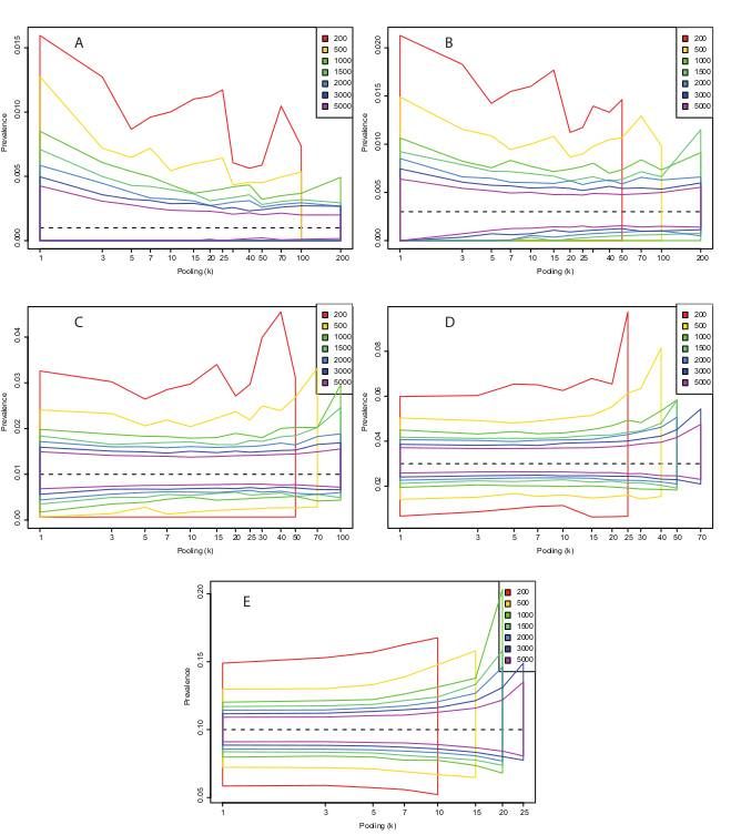
Abstract
Background: The number of con rmed COVID-19 cases divided by population size is used as a coarse
measurement for the burden of disease in a population. However, this fraction depends heavily on the
sampling intensity and the various test criteria used in different jurisdictions, and many sources indicate
that a large fraction of cases tend to go undetected. Methods: Estimates of the true prevalence of COVID-
19 in a population can be made by random sampling and pooling of RT-PCR tests. Here I use simulations
to explore how experiment sample size and degrees of sample pooling impact precision of prevalence
estimates and potential for minimizing the total number of tests required to get individual-level diagnostic
results.

Results: Sample pooling can greatly reduce the total number of tests required for prevalence estimation.
In low-prevalence populations, it is theoretically possible to pool hundreds of samples with only marginal
loss of precision. Even when the true prevalence is as high as 10% it can be appropriate to pool up to 15
samples. Sample pooling can be particularly bene cial when the test has imperfect speci city by
providing more accurate estimates of the prevalence than an equal number of individual-level tests.

Conclusion: Sample pooling should be considered in COVID-19 prevalence estimation efforts.

Background
It is widely accepted that a large fraction of COVID-19 cases go undetected. A crude measure of
population prevalence is the fraction of positive tests at any given date. However, this is subject to large
ascertainment bias since tests are typically only ordered from symptomatic cases, whereas a large
proportion of infected might show little to no symptoms [1,2]. Non-symptomatic infections can still shed
the Severe acute respiratory syndrome coronavirus 2 (SARS-CoV-2) virus and are therefore detectable by
reverse transcriptase polymerase chain reaction (RT-PCR)-based tests. It is therefore possible to test
randomly selected individuals to estimate the true disease prevalence in a population. However, if the
disease prevalence is low, very little information is garnered from each individual test. Under such
situations it can be advantageous to pool individual patient samples into a single pool [3-5]. Pooling
strategies, also called group testing, effectively increase the test capacity and reduces the required
number of RT-PCR-based tests. For SARS-CoV-2 pooling has been estimated to potentially reduce costs
by 69% [6], use ten-fold fewer tests [7] and clearing 20 times the number of people from isolation with the
same number of tests [8]. Note that I will not discuss pooling of SARS-CoV-2 antibody-based tests, since
there is currently not enough information about how pooling affects test parameters. However, sample
pooling has been successfully used for seroprevalence studies for other diseases such as human
immunode ciency virus (HIV) [9-11].

Methods

                                                  Page 2/12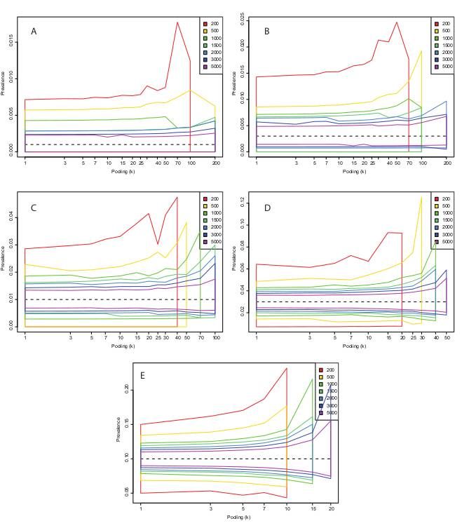
Due to technological limitations, the Methods section is only available as a download in the
supplementary les section.

Results
Estimates of prevalence

In the following, I use simulations to calculate the central 95% estimates of using tests with varying
sensitivity (0.7 and 0.95) and speci city (0.99 and 1.0) (Figs. 2-5). These estimates are based on the
initial pooled tests only, not the follow-up tests on sub-pools that allow for patient-level diagnosis.
(Including results from these samples would allow the precision from the pooled test estimates to
approach those of testing individually.) More samples are associated with a distribution of more narrowly
centered around the true value, while higher levels of pooling are generally associated with higher
variance in the estimates. The latter effect is less pronounced in populations with low prevalence. For
example, if the true population prevalence is 0.001 and a total of 500 samples are taken from the
population, the expected distribution of is nearly identical whether samples are run individually (k=1) or
whether they are run in pools of 25 (Figs. 2 or 4, panel A). Thus, it is possible to economize lab efforts by
reducing the required number of pools to be run from 500 to 20 (500 divided by 25) without any
signi cant alteration to the expected distribution of . At this prevalence and with this pooling level, 40
tests are su cient to get a correct patient-level diagnosis for all 500 individuals 97.5% of the time
(Supplementary Table 1). With 5000 total samples, the central estimates of vary little between individual
samples (95% interval 0.00021-0.0021) and a pooling level of 200 (95% interval 0.0022-0.0021). 145
reactions is enough to get patient-level diagnosis 97.5% of the time, in other words a reduction in the
number of separate RT-PCR setups by a factor of 34.5. (Supplementary Table 1)

The situation changes when the test speci city () is set to 0.99, that is, allowing for false positive test
results (Figs. 3, 5). This could theoretically occur from PCR cross-reactivity between COVID-19 and other
viruses, or from human errors in the lab. A problem with imperfect speci city tests are that false positives
typically outnumber true positives when the true prevalence is low. This creates a seemingly paradoxical
situation in which higher levels of sample pooling often leads to prevalence estimates that are more
accurate. This is because many pools test positive without containing a single true positive sample,
leading to in ated estimates of the prevalence. When the level of pooling goes up, the probability that a
positive pool contains at least one true positive sample increases, which increases the total precision.
The trends about appropriate levels of pooling for different sample numbers and levels of true population
prevalence are similar as for the perfect speci city scenario, but with imperfect speci city, we have an
added incentive for sample pooling in that prevalence estimates are closer to the true value with higher
levels of pooling. Even with a moderately accurate test (sensitivity 0.7 and speci city 0.99), when the
prevalence is 1%, pooling 50 together lets us diagnose 5000 individuals at the patient-level with a median
of 282 tests, a 17-fold reduction in the number of tests. This has virtually no in uence on our estimate of ,
and no signi cant effect on the number of wrongly diagnosed patients, which in both cases is about 1%.

                                                   Page 3/12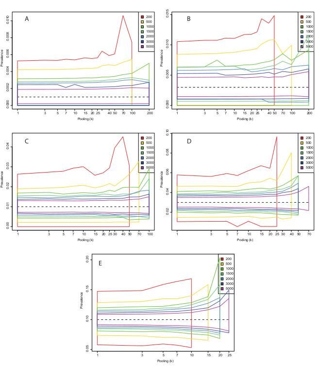
Discussion
The relationship between true prevalence, total sample number and level of pooling is not always
intuitive. Some combinations of parameters have serrated patterns for , which looks like Monte Carlo
errors (Figs 2-5). This is particularly true for the lower sample counts. However, this is not due to
stochasticity, but due to the discrete nature of each estimate of . That is, is not continuous and for small
pool sizes miniscule changes in the number of positive pools can affect the estimate quite a bit.

For example, if we take 200 samples and go with a pool size of 100, there are only three potential
outcomes: First, both pools are negative, in which case we believe the prevalence is 0. Second, one pool is
positive and the other negative, in which case we estimate as approximately 0.007 if the test sensitivity is
0.95. Finally, both pools are positive, in which case the formula of Cowling et al. does not provide an
answer because the fraction of positive pools is higher than the test sensitivity. This formula is only
intended to be used when the fraction of positive pools is much lower than the test sensitivity.

In general, very high levels of pooling are not appropriate since, depending on the true prevalence, the
probability that every single pool has at least one positive sample approaches 1. (Indicated by “NA” in
Supplementary Table 1). In low prevalence settings however, it can be appropriate to pool hundreds of
samples, but the total number of samples required to get a precise estimate of the prevalence is much
higher. Thus, decisions about the level of pooling need to be informed by the prior assumptions about
prevalence in the population, and there is a prevalence-dependent sweet spot to be found in the tradeoff
between precision and workload.

It is worth noting that the strategy I have outlined here does present some logistical challenges. Firstly,
samples must be allocated to pools in a random manner. This rules out some practical approaches such
as sampling a particular sub-district and pooling these, then sampling another district the next day.
Secondly, binary testing of sub-pools might be more cumbersome than it’s worth, in which case
Dorfman’s method should be preferred. Finally, there are major organizational challenges related to
planning and conducting such experiments across different testing sites and jurisdictions.

Conclusion
Attempts to estimate the true current prevalence of COVID-19 by PCR tests can bene t from sample
pooling strategies. Such strategies have the potential to greatly reduce the required number of tests with
only slight decreases in the precision of prevalence estimates. If the prevalence is low, it is generally
appropriate to pool even hundreds of samples, but the total sample count needs to be high in order to get
reasonably precise estimates of the true prevalence. On the other hand, if the prevalence is high there is
little to be gained by pooling more than 15 samples. Pooling strategies makes it possible to get patient-
level diagnostic information with only a fraction of the number of tests as individual testing. For a
prevalence of 10%, pooling cut the required number of tests by about two thirds, while for a prevalence of
0.1%, the number of required tests could on average be lowered by a factor of 50.

                                                  Page 4/12
Declarations
Ethics approval and consent to participate – Not applicable
Consent for publication – Not applicable
Availability of data and materials - Code written for this project is available at
https://github.com/admiralenola/pooledsampling-covid-simulation. All simulations and plots were
created in R version 3.2.3 [17].
Competing interests – Not applicable
Funding – Not applicable
Authors’ contributions – All work was done by OB
Acknowledgements – Not applicable
Abbreviations
HIV = Human immunode ciency virus
RT-PCR = Reverse transcriptase polymerase chain reaction
SARS-CoV-2 = Severe acute respiratory syndrome coronavirus 2
References
1. 1. Mizumoto K, Kagaya K, Zarebski A, Chowell G. Estimating the asymptomatic proportion of
coronavirus disease 2019 (COVID-19) cases on board the Diamond Princess cruise ship, Yokohama,
Japan, 2020. Eurosurveillance. 2020. doi:10.2807/1560-7917.es.2020.25.10.2000180
2. Q&A: Similarities and differences – COVID-19 and in uenza. [cited 17 Apr 2020]. Available:
https://www.who.int/news-room/q-a-detail/q-a-similarities-and-differences-covid-19-and-in uenza
3. Hogan CA, Sahoo MK, Pinsky BA. Sample Pooling as a Strategy to Detect Community Transmission
of SARS-CoV-2. JAMA. 2020. doi:10.1001/jama.2020.5445
4. Dorfman R. The detection of defective members of large populations. The Annals of Mathematical
Statistics 1943;14(4): 436-440
5. Cherif A, Grobe N, Wang X, Kotanko P. Simulation of Pool Testing to Identify Patients With
Coronavirus Disease 2019 Under Conditions of Limited Test Availability. JAMA Network Open. 2020
Jun 1;3(6):e2013075-.
6. Abdalhamid B, Bilder CR, McCutchen EL, Hinrichs SH, Koepsell SA, Iwen PC. Assessment of specimen
pooling to conserve SARS CoV-2 testing resources. American journal of clinical pathology. 2020 May
5;153(6):715-8.
Page 5/127. Verdun CM, Fuchs T, Harar P, Elbrächter D, Fischer DS, Berner J, Grohs P, Theis FJ, Krahmer F. Group
testing for SARS-CoV-2 allows for up to 10-fold e ciency increase across realistic scenarios and
testing strategies. medRxiv. 2020 May 13.
8. Gollier C, Gossner O. Group testing against Covid-19. Covid Economics. 2020 Apr 8;2.
9. Cahoon-Young B, Chandler A, Livermore T, Gaudino J, Benjamin R. Sensitivity and speci city of
pooled versus individual sera in a human immunode ciency virus antibody prevalence study.
Journal of Clinical Microbiology. 1989 Aug 1;27(8):1893-5.
10. Kline RL, Brothers TA, Brookmeyer R, Zeger S, Quinn TC. Evaluation of human immunode ciency
virus seroprevalence in population surveys using pooled sera. Journal of clinical microbiology. 1989
Jul 1;27(7):1449-52.
11. Behets F, Bertozzi S, Kasali M, Kashamuka M, Atikala L, Brown C, Ryder RW, Quinn TC. Successful
use of pooled sera to determine HIV-1 seroprevalence in Zaire with development of cost-e ciency
models. Aids. 1990 Aug 1;4(8):737-42.
12. Corman VM, Landt O, Kaiser M, Molenkamp R, Meijer A, Chu DK, et al. Detection of 2019 novel
coronavirus (2019-nCoV) by real-time RT-PCR. Euro Surveill. 2020;25. doi:10.2807/1560-
7917.ES.2020.25.3.2000045
13. Yelin I, Aharony N, Shaer-Tamar E, Argoetti A, Messer E, Berenbaum D, et al. Evaluation of COVID-19
RT-qPCR test in multi-sample pools. medRxiv. 2020; 2020.03.26.20039438.
14. Tu XM, Litvak E, Pagano M. Screening tests: Can we get more by doing less?. Statistics in Medicine.
1994 Oct 15;13(19‐20):1905-19.
15. Cowling DW, Gardner IA, Johnson WO. Comparison of methods for estimation of individual-level
prevalence based on pooled samples. Prev Vet Med. 1999;39: 211–225.
16. Theagarajan LN. Group Testing for COVID-19: How to Stop Worrying and Test More. arXiv preprint
arXiv:2004.06306. 2020 Apr 14.
17. R Core Team. R: a language and environment for statistical computing. Vienna, Austria: R
Foundation for Statistical Computing; 2013.
Supplementary Information
Supplementary Table 1 – Table containing prevalence estimates and, the estimated required number of
tests, and the expected proportion incorrectly classi ed patients for all parameter combinations. Se =
sensitivity. Sp = speci city. N = number of samples. k = pooling level. P = true prevalence. p 2.5%, p 50.0%,
p 97.5% = 2.5, 50 and 97.5 quantile of estimated prevalence. T 2.5%, T 50.0%, T 97.5% = 2.5, 50 and 97.5
quantile of estimated number of tests required to get individual-level diagnoses. E(S) = Expected number
of tests saved when compared to testing individually for this N. E(inc) = Expected percentage of patients
that are diagnosed incorrectly at this parameter combination. [Excel le]
Supplementary document 1 – Testing for freedom from disease and distinguishing a disease-free
population from a low-prevalence one.
Page 6/12Fig. S1 – Testing for freedom of disease with a test with perfect speci city. The x-axis represents
different true levels of , and the colored lines represent the number of samples associated with 95%
probability of having at least one positive sample at that prevalence level. For perfect speci city tests this
is commonly interpreted as meaning that we can be 95% certain that the true prevalence is lower. The
effects of sample pooling are explored with different color lines. Panel A: Test speci city = 1.0; Panel B:
Test speci city = 0.99.
Fig. S2 – Using a test with speci city of 0.99 to discriminate a disease-free population from a population
with with 2743 samples from both populations. Panel A: The expected number of positive samples from
the disease-free and the low-prevalence populations; Panel B: The probability mass function of the
difference in the number of positive samples between the low-prevalence and the disease-free population.
With 2743 samples from both populations, there is a 5% probability of getting more positive tests from
the disease-free population.
Figures
Figure 1
Algorithm used to minimize the number of RT-PCR reactions in pooled sampling. Negative pools regard
all constituent patient samples as negative, whereas positive pools are split in two, and the process
repeated. Red circle = Pool testing positive. Grey circle = Pool testing negative. Red/grey squares = Patient
samples in pool, with color indicating diseased/non-diseased status.
Page 7/12Figure 2
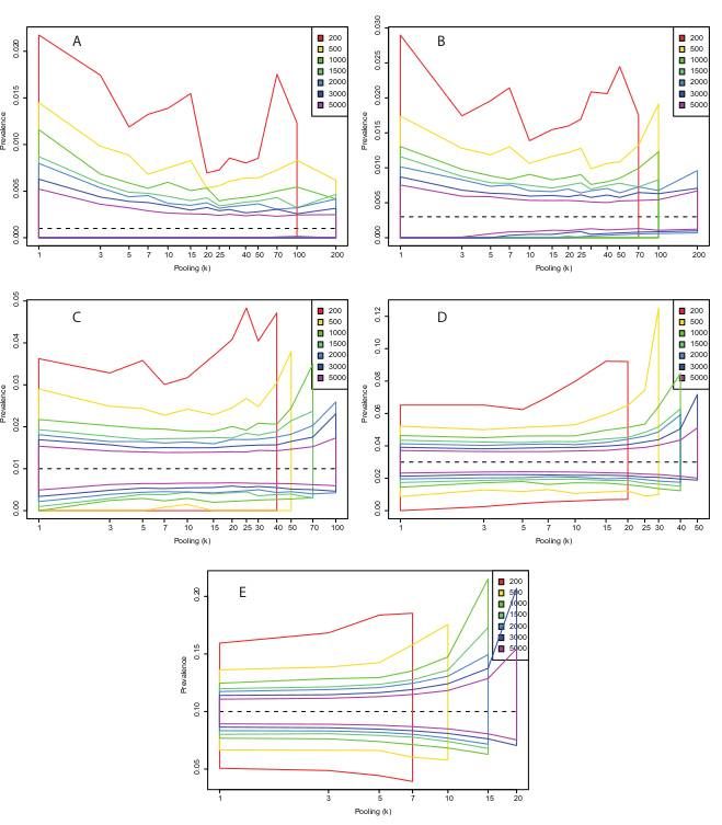
Central 95% estimates of p ̂ with a test with sensitivity (η) 0.95 and perfect speci city (θ=1) under
different combinations of total number of samples and level of sample pooling. Panel A: p=0.001; Panel
B: p=0.003; Panel C: p=0.01; Panel D: p=0.03; Panel E: p=0.10
Page 8/12Figure 3
Central 95% estimates of p ̂ with a test with sensitivity (η) 0.95 and a speci city (θ) of 0.99 under
different combinations of total number of samples and level of sample pooling. Panel A: p=0.001; Panel
B: p=0.003; Panel C: p=0.01; Panel D: p=0.03; Panel E: p=0.10
Page 9/12Figure 4
Central 95% estimates of p ̂ with a test with sensitivity (η) 0.70 and perfect speci city (θ=1) under
different combinations of total number of samples and level of sample pooling. Panel A: p=0.001; Panel
B: p=0.003; Panel C: p=0.01; Panel D: p=0.03; Panel E: p=0.10
Page 10/12Figure 5
Central 95% estimates of p ̂ with a test with sensitivity (η) 0.70 and a speci city (θ) of 0.99 under
different combinations of total number of samples and level of sample pooling. Panel A: p=0.001; Panel
B: p=0.003; Panel C: p=0.01; Panel D: p=0.03; Panel E: p=0.10
Supplementary Files
Page 11/12This is a list of supplementary les associated with this preprint. Click to download.
COVID19SUPPLMERGEDCHANGES.docx
RESTABLE.xls
FigS2.pdf
FigS1.pdf
Methods.docx
Page 12/12You can also read