Critical loads for eutrophication and acidification for European terrestrial ecosystems 03/2021

DOKUMENTATIONEN

 03/2021
 Critical loads for
 eutrophication and
 acidification for
 European terrestrial
 ecosystems
 Final report

German Environment Agency

DOKUMENTATIONEN 03/2021

Ressortforschungsplan of the Federal Ministry for the
Enviroment, Nature Conservation and Nuclear Safety

Project No. (FKZ) 3719 52 201 0
Report No. (UBA-FB) FB000514/ENG

Critical loads for eutrophication and
acidification for European terrestrial
ecosystems
Final report

by
Gert Jan Reinds, Daphne Thomas
Wageningen University and Research, Environmental Research,
Wageningen (Netherlands)
Maximilian Posch
International Institute for Applied Systems Analysis, Laxenburg (Austria)
Jaap Slootweg
National Institute for Public Health and the Environment, Bilthoven (Netherlands)

On behalf of the German Environment Agency

Imprint

Publisher
Umweltbundesamt
Wörlitzer Platz 1
06844 Dessau-Roßlau
Tel: +49 340-2103-0
Fax: +49 340-2103-2285
buergerservice@uba.de
Internet: www.umweltbundesamt.de

 /umweltbundesamt.de
 /umweltbundesamt

Report performed by:
Wageningen Environmental Research
PO Box 47
6700 AA Wageningen
Netherlands

Report completed in:
January 2021

Edited by:
Section II 4.3 Air Pollution and Terrestrial Ecosystems
Christin Loran

Publication as pdf:
http://www.umweltbundesamt.de/publikationen

ISSN 1862-4804

Dessau-Roßlau, July 2021

The responsibility for the content of this publication lies with the author(s).

DOKUMENTATIONEN Critical loads for eutrophication and acidification for European terrestrial ecosystems – Final report

Abstract: Critical loads for eutrophication and acidification for European terrestrial ecosystems
In this final report of the project “Critical loads for eutrophication and acidification for European
terrestrial ecosystems” a description is given of the datasets used to construct a database that
can be used as a basis for critical load computations. Datasets are described in general terms.
Furthermore, the derivation of input data for the critical load models is described in detail. Next,
a description is given of an R package and R scripts that can be used for these critical load
computations. Both the installation of the scripts as well as their functioning is described and so
are the associated data. Thereafter, a ‘validation’ is given of the R package and R scripts. Results
are validated against the 2017 results from the Fortran based background data base
computations of RIVM-CCE. Furthermore, a comparison is made with national critical load data
submitted to the CCE by Ireland and Germany. Finally, critical loads related to the eutrophying
effects of nitrogen are compared to empirical critical loads of nitrogen.

Kurzbeschreibung: Ökologische Belastungsgrenzen (Critical Loads) für eutrophierende und
versauernde Einträge für europäische land-basierte Ökosysteme
Dieser Endbericht des Projekts „Critical loads for eutrophication and acidification for European
terrestrial ecosystems” beschreibt die Datensätze, die verwendet wurden um eine Datenbank zu
generieren, die als Grundlage für die Berechnung von Critical Loads genutzt werden kann. Die
einzelnen Datensätze werden nur allgemein beschrieben, während die Herleitung der
Eingabedaten für die Critical Loads Modelle im Detail beschrieben werden. Im Weiteren werden
R-Scripte und ein R Programmpaket beschrieben, die für die Critical Loads Berechnungen
verwendet werden können. Sowohl die Installation der R-Scripte als auch deren Funktionsweise
werden beschrieben. Des Weiteren wird eine ‚Validierung‘ der R-Scripte und des R
Programmpakets präsentiert. Resultate werden verglichen mit den Resultaten, die 2017 mit
einer Fortran-basierten Software vom RIVM-CCE generiert wurden. Auch ein Vergleich wird
durchgeführt mit nationalen Critical Loads Daten, die 2017 von Irland und Deutschland zum
RIVM-CCCE transferiert wurden. Schlussendlich werden die berechneten eutrophierenden
Critical Loads mit empirischen Critical Loads für Stickstoff verglichen.

 5

DOKUMENTATIONEN Critical loads for eutrophication and acidification for European terrestrial ecosystems – Final report

Table of content
Table of content ...................................................................................................................................... 6
List of figures ........................................................................................................................................... 8
List of tables .......................................................................................................................................... 10
List of abbreviations .............................................................................................................................. 10
Summary ............................................................................................................................................... 12
Zusammenfassung................................................................................................................................. 15
1 Introduction................................................................................................................................... 18
 1.1 Contents of the report .......................................................................................................... 19
2 Geographical data ......................................................................................................................... 20
 2.1 Land cover ............................................................................................................................. 20
 2.2 Soils ....................................................................................................................................... 23
 2.3 Forest growth regions ........................................................................................................... 24
 2.4 Distance to coast ................................................................................................................... 24
 2.5 Natura 2000 areas ................................................................................................................. 24
 2.6 Base cation deposition .......................................................................................................... 24
 2.7 Meteorological data and hydrology...................................................................................... 26
 2.8 Overlay procedure ................................................................................................................ 26
 2.8.1 General procedure ............................................................................................................ 26
 2.8.2 Details of the ArcGIS procedures ...................................................................................... 26
3 Input data for the critical load model ........................................................................................... 29
 3.1 Simple Mass Balance (SMB) critical load equations ............................................................. 29
 3.1.1 Introduction ...................................................................................................................... 29
 3.1.2 The critical load of nutrient N ........................................................................................... 29
 3.1.3 Critical loads of N and S acidity ......................................................................................... 29
 3.2 Parameters for computing ANC (Acid Neutralising Capacity)............................................... 30
 3.2.1 Aluminium ......................................................................................................................... 30
 3.2.2 Bicarbonate ....................................................................................................................... 30
 3.2.3 Organic acids ..................................................................................................................... 30
 3.3 Soil parameters ..................................................................................................................... 31
 3.3.1 Thickness of the rooting zone ........................................................................................... 31
 3.3.2 Denitrification fraction...................................................................................................... 31
 3.3.3 Weathering rates of base cations ..................................................................................... 32
 3.3.4 Nitrogen immobilization ................................................................................................... 32
 6

DOKUMENTATIONEN Critical loads for eutrophication and acidification for European terrestrial ecosystems – Final report

 3.4 Uptake of nitrogen and base cations .................................................................................... 33
4 Methodological approach for computing critical loads ................................................................ 34
 4.1 Workflow for computing critical loads.................................................................................. 34
 4.2 The BGDB package ................................................................................................................ 34
 4.3 The BGRUN scripts ................................................................................................................ 35
 4.3.1 Meteorological data for the MetHyd model..................................................................... 35
 4.3.2 Computing critical loads for Europe: MainLoop.R ............................................................ 38
 4.4 Verification of the results...................................................................................................... 38
5 Computing critical loads using the R software .............................................................................. 40
 5.1 Setting up the R environment ............................................................................................... 40
 5.2 Preparing the meteorological data ....................................................................................... 41
 5.3 Running the critical load model: MainLoop.R....................................................................... 42
 5.4 Verification of the R procedures ........................................................................................... 45
6 Comparison with 2017 background data base results .................................................................. 47
7 Comparison of critical loads with national data from Ireland and Germany ................................ 53
 7.1 Introduction .......................................................................................................................... 53
 7.2 Ireland ................................................................................................................................... 53
 7.3 Germany................................................................................................................................ 57
8 Comparison of computed critical loads of eutrophication (or nutrient N) to empirical critical
 loads .............................................................................................................................................. 62
 8.1 Introduction .......................................................................................................................... 62
 8.2 Method.................................................................................................................................. 62
 8.3 Results ................................................................................................................................... 62
9 Conclusions.................................................................................................................................... 67
10 References ..................................................................................................................................... 68
A Appendices .................................................................................................................................... 71
 A.1 Soil characteristics in the upper 50 cm of the soil as a function of soil type: median
 values for soil pH, soil organic carbon content, soil N content, soil carbonate content ,
 and the number of observations the median value is based on. ......................................... 71
 A.2 Documentation of the package BGDB .................................................................................. 74
 A.3 Conversion of radiation data ................................................................................................ 75
 A.4 Area (in km2) and number of receptors per country and EUNIS class in the critical load
 database ................................................................................................................................ 77

 7

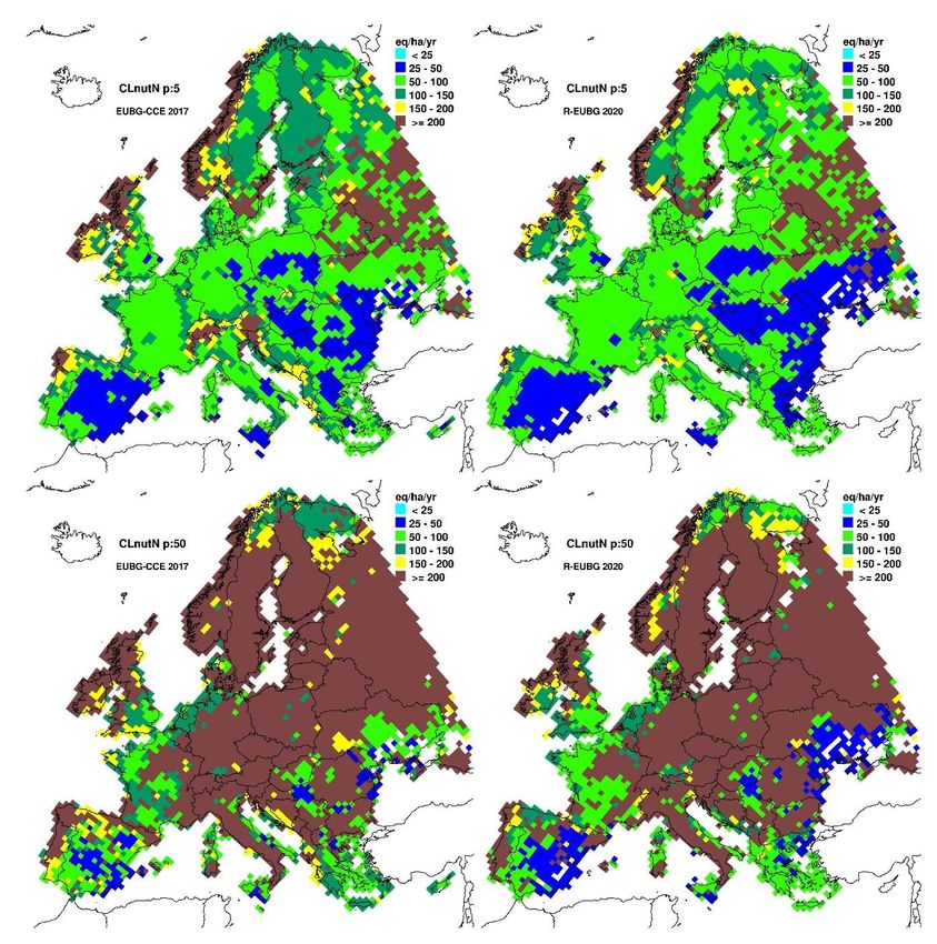
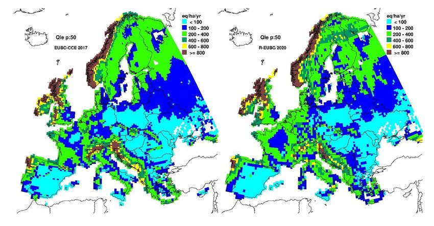
DOKUMENTATIONEN Critical loads for eutrophication and acidification for European terrestrial ecosystems – Final report

List of figures
Figure 1: Input form for the ArcGIS procedure to process the soil data ................. 26
Figure 2: Progress window ...................................................................................... 28
Figure 3a: Comparison of the cumulative distribution of daily values for rainfall
 (upper 6 graphs) and rainfall (lower six graphs) for 4 months
 (1,4,7,10) at 2 locations in 3 selected 0.5 × 0.5˚ cells in Europe
 .................................................................................................. 37
Figure 4: Verification of the R procedures .............................................................. 45
Figure 5: Median Calcium deposition (Cadep) in eq/ha/yr for the 2017 background
 DB (left) and the EUDB 2020 (right) ......................................... 47
Figure 6: Median Magnesium deposition (Mgdep) in eq/ha/yr for the 2017
 background DB (left) and the EUDB 2020 (right) ..................... 48
Figure 7: Median Calcium weathering (Cawe) in eq/ha/yr for the 2017 background
 DB (left) and the EUDB 2020 (right) ......................................... 49
Figure 8: Median precipitation surplus (leaching flux; Qle) in mm/yr for the 2017
 background DB (left) and the EUDB 2020 (right) ..................... 49
Figure 9: Cumulative distribution function (CDF) of CLminN in eq/ha/yr for the
 2017 background DB (green line) and EUDB 2020 (blue line).. 50
Figure 10: 5-th percentile (upper row) and median (lower row) CLmaxS in
 eq/ha/yr for the 2017 background DB (left) and the EUDB 2020
 (right) ........................................................................................ 51
Figure 11: 5-th percentile (upper row) and median (lower row) CLnutN in eq/ha/yr
 for the 2017 background DB (left) and the EUDB 2020 (right) 52
Figure 12: CDFs of CLmaxS for forests (EUNIS ‘G’; left) and non-forests (all other
 classes) in Ireland taken from the 2017 NFC data (green lines)
 and the 3 Runs of the new EUDB 2020 (blue lines; see text for
 their definition)......................................................................... 55
Figure 13: CDFs of CLminN for forests (EUNIS ‘G’; left) and non-forests (all other
 classes) taken in Ireland from the 2017 NFC data (green lines)
 and the new EUDB 2020 (blue lines) ........................................ 56
Figure 14: CDFs of CLmaxN for forests (EUNIS ‘G’; left) and non-forests (all other
 classes) in Ireland taken from the 2017 NFC data (green lines)
 and the 3 Runs of the new EUDB 2020 (blue lines; see text for
 their definition)......................................................................... 56
Figure 15: CDFs of CLnutN/CLeutN for forests (EUNIS ‘G’; left) and non-forests (all
 other classes) in Ireland taken from the 2017 NFC data (green
 lines) and the new EUDB 2020 (blue lines) .............................. 57
Figure 16: CDFs of CLmaxS for forests (EUNIS ‘G’; left) and non-forests (all other
 classes) in Germany taken from the 2017 NFC data (green
 lines) and the new EUDB 2020 (blue lines) .............................. 58
Figure 17: CDFs of CLminN for forests (EUNIS ‘G’; left) and non-forests (all other
 classes) in Germany taken from the 2017 NFC data (green
 lines) and the new EUDB 2020 (blue lines) .............................. 59
 8

DOKUMENTATIONEN Critical loads for eutrophication and acidification for European terrestrial ecosystems – Final report

Figure 18: CDFs of long-term net N immobilisation (Nimm, top) and net N uptake
 (Nupt, bottom) for forests (EUNIS ‘G’; left) and non-forests (all
 other classes) in Germany taken from the 2017 NFC data
 (green lines) and the new EUDB 2020 (blue lines) ................... 59
Figure 19: CDFs of CLmaxN for forests (EUNIS ‘G’; left) and non-forests (all other
 classes) in Germany taken from the 2017 NFC data (green
 lines) and the new EUDB 2020 (blue lines) .............................. 60
Figure 20: CDFs of CLnutN/CLeutN for forests (EUNIS ‘G’; left) and non-forests (all
 other classes) in Germany taken from the 2017 NFC data
 (green lines) and the new EUDB 2020 (blue lines) ................... 61
Figure 21: Median values for CLnutN from EUDB 2020 (green) and the average
 empirical critical loads for N (blue) in kg.ha-1.yr-1 for the various
 EUNIS classes ............................................................................ 65
Figure 22: Daily solar downward radiation in W/m2 at the Wageningen grid cell:
 (a) for the years 1999 (blue), 2009 (green), and 2018 (red); (b)
 the daily 20-year (1999-2018) minimum and maximum daily
 downward radiation, expressed in MJ/m2/. The red and orange
 curves show the daily radiation for nj=0 (no sunshine) and nj=1
 (=100% sunshine) as computed by eq.B4 (see below) ............. 75

 9

DOKUMENTATIONEN Critical loads for eutrophication and acidification for European terrestrial ecosystems – Final report

List of tables
Table 1: EUNIS codes and description .....................................................................20
Table 2: Texture class definition.............................................................................. 23
Table 3: Regression coefficient for computing Mg deposition ............................... 25
Table 4: Texture class (see Table 2 for definitions) dependent constants for
 estimating DOC ......................................................................... 31
Table 5: Dominant annual water regimes ............................................................... 31
Table 6: Weathering rates of separate base cations as a fraction of the total
 weathering rate ........................................................................ 32
Table 7: R routines in the BGDB package ................................................................ 34
Table 8: Files and directories for the BGRUN script ................................................ 35
Table 9: iAci values and their associated criterion .................................................. 42
Table 10: Parameters in the output file of the critical load procedure (MainLoop);
 all in eq/ha/yr unless said otherwise........................................ 44
Table 11: Number of sites and ecosystem areas in Ireland for the Level-1 EUNIS
 classes in the 2017 NFC data and the new EUDB 2020 ............ 53
Table 12: FAO soil types in Ireland and ecosystem area which they cover in EUDB
 2020 .......................................................................................... 54
Table 13: Number of sites and ecosystem areas in Germany for the Level-1 EUNIS
 classes in the 2017 NFC data and the new EUDB 2020 ............ 58
Table 14: SMB critical loads (5, 50 and 95 percentile) using the [N]acc criterium for
 northern Europe and empirical critical loads (lower value of the
 range, upper value and mean) in kg N.ha-1 .............................. 63
Table 15: SMB critical loads (5, 50 and 95 percentile) using the [N]acc criterium for
 western Europe and empirical critical loads (lower value of the
 range, upper value and average) in kg N.ha-1........................... 64

List of abbreviations
 ANC Acid Neutralizing Capacity
 Bc Base cations (Ca+Mg+K)
 BC Base cations (Bc+Na)
 CCE Coordination Centre for Effects
 CEC Cation Exchange Capacity
 CL Critical Load
 CDF Cumulative Distribution Function
 EUDB European Data Base for critical loads
 EUNIS European Nature Information System
 ICP M&M International Cooperative Programme on Modelling and Mapping
 LRTAP (Convention on) Long-range Transboundary Air Pollution
 10

DOKUMENTATIONEN Critical loads for eutrophication and acidification for European terrestrial ecosystems – Final report

 ANC Acid Neutralizing Capacity
 N Nitrogen
 RIVM Rijksinstituut voor Volksgezondheid en Milieu (NL)
 S Sulphur
 SMB Simple Mass Balance
 UBA Umweltbundesamt (German Environment Agency)
 UNECE United Nations Economic Commission for Europe
 WGE Working Group on Effects (under the LRTAP Convention)

 11

DOKUMENTATIONEN Critical loads for eutrophication and acidification for European terrestrial ecosystems – Final report

Summary
As a result of the observed relationship between air pollution and acidification of soils and
waters, the United Nations Economic Commission for Europe (UNECE) initiated in 1979 the
Convention on Long-range Transboundary Air Pollution (LRTAP). Under the Working Group on
Effects (WGE), the ICP on Modelling and Mapping of Critical Levels and Loads and Air Pollution
Effects (ICP M&M) is responsible for the assessment of regional critical loads. Critical loads for
acidity and eutrophication are commonly modelled with simple mass balance (SMB) models. In
integrated assessments, critical loads are used to compute cost-effective emission abatement
measures based on ecosystem vulnerability (expressed by these critical loads) and emission
abatement costs, optimized in a European framework. Critical loads are therefore an important
input for (European) air pollution policies.

A main task of the Coordination Centre for Effects (CCE), the data centre of the ICP on Modelling
& Mapping, is to collect and collate national data on critical loads (CLs), and to provide European
maps and databases to the relevant bodies under the LRTAP Convention. For meaningful
applications, a complete European coverage with CLs is desirable/required. If a country did not
contribute national data, the former CCE at RIVM in the Netherlands filled the gaps with CLs
from a so-called European Background Database (EU-DB) of critical loads, which was
maintained (and regularly updated) by the CCE in collaboration with Wageningen
Environmental Research.

After the CCE was transferred from the RIVM to the UBA in 2018, a revision of the existing
background database was required. Therefore, Wageningen Environmental Research was
commissioned to develop a database and computational procedures to compute critical loads for
eutrophication (by nitrogen) and acidification (by nitrogen and sulphur) for terrestrial
ecosystems in Europe.

In the new system, the following critical loads for N and S were computed with the Simple Mass
Balance (SMB) method: the maximum critical load for sulphur (CLmaxS), the minimum critical
load for nitrogen (CLminN), the maximum critical load for nitrogen (CLmaxN) and the critical
load for nutrient nitrogen (CLnutN). CLmaxS can be based on critical values for various chemical
criteria such as molar [Al]:[Bc] ratio in soil solution, pH or base saturation.

To compute critical load for (semi-)natural ecosystems, information is needed on ecosystem
characteristics such as vegetation cover and soil. We therefore combined six maps to construct a
background data base for critical load computations: (1) Land cover, (2) Soil type, (3) Forest
growth region, (4) Distance to coast, (5) Natura 2000 delineations, (6) Country borders. Critical
load computations we restricted to (semi) natural habitats, i.e. forests and (semi-)natural
vegetation (mires, bogs and fens, natural grasslands and heathland, scrub and tundra).

These maps were gridded in an ArcMap Pro procedure in Python to rasters with a resolution of
0.01° × 0.01° for each country separately. Thereafter, the different layers were combined
(overlayed). There are also two regional data sets used: base cation deposition and
meteorological data (temperature and precipitation surplus). Precipitation surpluses were
computed using the MetHyd model, which was run for the period 1999-2018 using daily
meteorological data.

 12

DOKUMENTATIONEN Critical loads for eutrophication and acidification for European terrestrial ecosystems – Final report

A set of R procedures (called EUDB 2020) was developed to compute the critical loads for
Europe. The software consists of two parts: (a) the BGDB package that holds the basic routines
such as transfer functions, conversion functions and the critical load routine and (b) the BGRUN
scripts to process the meteorological data, compute the hydrology and the ‘MainLoop’ that
combines all data and scripts to compute critical loads for a set of countries. In ‘MainLoop’ the
following sequence of computations is made:

 a. Read the input data from the map overlays on soil types, vegetation type, forest
 growth region etc.

 b. Read in input data from plain ASCII files such as forest growth and soil data

 c. Make all the necessary conversions (e.g. compute bulk density from soil
 characteristics)

 d. Prepare the meteorological data for use in MetHyd by, e.g., filling the gaps due to
 missing data

 e. Run the MetHyd model

 f. Run the critical load model

Critical loads are computed in ‘stripes’ of 0.5 degrees latitude. The MainLoop runs from south to
north through Europe preparing meteorological data, computing hydrology and critical loads for
all receptors in the latitude stripe of 0.5 degrees and between -12 and 42 degrees longitude.

Results from the R procedure have been mapped and compared to the results from the
background critical loads computed by RIVM-CCE and reported in the CCE Final Report 2017.
Compared to the 2017 results a few changes have been made regarding the computation of
critical loads:

 1. The software was ported to R

 2. The MetHyd model uses daily data for 1999-2018 instead of monthly data 1970-2000

 3. The Efiscen forest growth data have been updated to the latest (2016) version

Due to these changes, some minor differences occur in inputs (precipitation surplus) and in
critical loads between the new EUDB 2020 and the 2017 results, but the patterns over Europe
are mostly (almost) identical.

National critical load data bases provided in 2017 by the Irish and German NFCs have been
compared with the CLs for those countries generated by EUDB 2020, with a focus on a
comparison of ecosystem areas and the critical loads of N and S. Due to the use of regional maps
and differences in ecosystem classification, ecosystem areas deviate between national data and
EUDB 2020. Since both Ireland and Germany have used methods for computing critical loads
that deviate from the ‘standard’, also critical loads differ from EUDB. For Ireland critical loads
from EUDB 2020 are close to the national ones if we adapt the R software such that it ‘mimics’
the way the national CLs were computed. For Germany, national critical loads have been

 13

DOKUMENTATIONEN Critical loads for eutrophication and acidification for European terrestrial ecosystems – Final report

computed using various criteria (pH, Bsat, Al/Bc, no Al depletion) and various critical values for
each of these criteria (e.g. critical base saturation between 3% and 62% and critical pH between
4.08 and 6.2) in many classes. Since the assignment of criteria and their values was based on
national maps of soils and vegetation, it was not possible to mimic this in EUDB 2020.

Critical loads for eutrophying nitrogen (CLnutN) from EUDB 2020 were compared to empirical
critical loads for N. ClnutN values consist of N uptake, critical N leaching, long-term N
immobilisation and N denitrification. Empirical critical N loads are mostly based on observed
changes in the structure and functioning of ecosystems in field studies, and relate to unwanted
changes in species abundance, -composition and/or -diversity (‘ecosystem structure’), or to N
leaching, -decomposition or -mineralisation rate (‘ecosystem functioning’),

From the above two definitions, it is clear that although both critical loads mainly relate to the
eutrophying effects of N, they are conceptually different. The SMB critical load has a strong
leaching component: for non-forests for example, net uptake is set to zero, acceptable N
immobilisation is a low, constant, value for all EUNIS classes, so N leaching is the main term in
the computation of CLnutN. For empirical critical loads, the mentioned changes in species
abundance, composition and/or diversity may be caused by N enrichment in the soil organic and
mineral phase without resulting in enhanced N leaching. Two runs with EUDB 2020 were made,
one with a critical N concentration of 0.2 mg N.l-1 for conifers forest and 0.3 mg N.l-1 for
deciduous forests and semi-natural vegetations (which are the standard values from the
Mapping Manual) and a second run with values of 3 mg N.l-1 for conifers and deciduous forests
and 3.5 mg N.l-1 for seminatural vegetations. The latter run used critical values thought to be
representative for vegetation changes in Western Europe.

When using the strict values for the critical N concentration, SMB based CLnutN varies mostly
between 1-3 and 10-15 kg N.ha-1. Compared to empirical critical loads, the median value is
mostly still lower than the lower end of the empirical range. Ecosystems that occur in areas with
a very high precipitations surplus (and thus a much higher N leaching) can have very high
critical loads. When using the higher values for the critical N concentration, median values for
CLnutN compare quite well with the average values of the empirical range, especially for forest
ecosystems. For some non-forest ecosystems, such as ‘Alpine grasslands’ and ‘Tundras’, the
median CLnutN is much higher than the upper value of the empirical range. In high precipitation
areas, the criterion for the critical N concentration of 2-3 mgN.l-1 leads to unrealistically high
critical loads.

 14

DOKUMENTATIONEN Critical loads for eutrophication and acidification for European terrestrial ecosystems – Final report

Zusammenfassung
Aufgrund des beobachteten Zusammenhangs zwischen Luftverschmutzung (durch Schwefel und
Stickstoff) und der Versauerung von Böden und Gewässern rief die United Nations Economic
Commission for Europe (UNECE) im Jahre 1979 das Genfer Luftreinhalteabkommen (LRTAP
Convention) ins Leben. Als Teil der Working Group on Effects (WGE) unter der LRTAP
Convention ist das ICP on Modelling and Mapping of Critical Levels and Loads and Air Pollution
Effects (ICP M&M) verantwortlich für die Herleitung und Anwendung von ökologischen
Belastungsgrenzen (Critical Loads). Critical Loads (CLs) für versauernde und eutrophierende
Einträge werden gewöhnlich mit einfachen Massebilanzmodellen (Simple Mass Balance (SMB)
models) berechnet. Integrierte Bewertungen (integrated assessments) werden herangezogen
um kosteneffektive Emissionsreduktionen zu ermitteln. Diese basieren auf der Sensitivität von
Ökosystemen (ausgedrückt durch deren Critical Loads) und den Kosten von
Reduktionsmaßnahmen, optimiert in einem europäischen Zusammenhang. Critical Loads sind
daher ein wichtiger Input für die (europäische) Luftreinhaltepolitik.

Eine Hauptaufgabe des Coordination Centre for Effects (CCE), das Datenzentrum des ICP M&M,
ist es nationale CL-Daten zu sammeln, daraus europäische CL-Karten, Datenbanken und
Statistiken zu generieren und den relevanten Körperschaften der LRTAP Convention zur
Verfügung zu stellen. Für sinnvolle Anwendungen sind vollständige CL-Karten wünschenswert
bzw. erforderlich. Für Länder, die keine CL-Daten zur Verfügung stellten, wurden die Lücken
vom früheren CCE (beim RIVM in den Niederlanden) mit CLs der sogenannten ‚European
Background Database‘ (EU-DB) gefüllt. Diese EU-DB wurde von jenem CCE unterhalten und
immer wieder aktualisiert, in Zusammenarbeit mit dem ‚Wageningen Environmental Research‘
Institut.

Nach dem Transfer des CCE zum UBA im Jahr 2018 wurde eine Revision dieser Datenbank (EU-
DB) erforderlich. Daher wurde das ‚Wageningen Environmental Research‘ Institut beauftragt
eine Datenbank und Computerprogramme zu entwickeln, die es erlauben Critical Loads für
Eutrophierung (durch Stickstoff, N) und Versauerung (durch N und Schwefel, S) für landbasierte
Ökosysteme in Europa zu berechnen.

Mit dieser neuen Software wurden die folgenden Critical Loads mit SMB Modellen berechnet:
der maximale CL für Schwefel (CLmaxS), der minimale und maximale CL für Stickstoff (CLminN
und CLmaxN) und der CL für eutrophierendes N (CLnutN). CLmaxS kann für verschiedene
chemische Kriterien berechnet werden, z.B. molares [Al]:[Bc] Verhältnis in Bodenlösung, pH
oder Basensaturation.

Um Critical Loads für Ökosysteme zu berechnen werden Daten über die Charakteristika dieser
Ökosystem benötigt, wie z.B. räumliche Ausdehnung der Vegetation sowie Eigenschaften der
Böden. Daher wurden die folgenden sechs Karten kombiniert um eine Grundlage für die
Berechnung von CLs zu schaffen: (1) Landbedeckung, (2) Bodentyp, (3) Waldwuchsregionen, (4)
Abstand zur Küste, (5) Natura 2000 Gebiete, und (6) Staatsgrenzen. Die Berechnung von CLs
beschränkte sich auf naturnahe Ökosystem (Habitate), d.h. Wälder, Moore und andere
Feuchtgebiete, naturnahes Gras- und Heideland, Buschland und Tundra.

Die Dateninhalte dieser Karten wurden – separat für jedes Land – mit einer ArcMap Pro
Prozedur (geschrieben in Python) auf ein Gitter der Dimension 0.01° × 0.01° projiziert und
überlappt (kombiniert). Auch zwei weitere, schon gerasterte, europäische Datensätze wurden

 15

DOKUMENTATIONEN Critical loads for eutrophication and acidification for European terrestrial ecosystems – Final report

herangezogen: die Deposition basischer Kationen und meteorologische/hydrologische Daten
(Temperatur und Niederschlagsüberschuss). Niederschlagsüberschüsse wurden mit dem
MetHyd-Modell für die Periode 1999-2018 berechnet, unter Verwendung täglicher
meteorologischer Daten.

Um Critical Loads für Europa zu berechnen wurde eine R-Umgebung (genannt ‚EUDB 2020‘)
entwickelt. Diese besteht aus zwei Teilen: (a) dem BGDB Paket, welches die elementaren
Routinen (Unterprogramme) enthält, wie z.B. Transferfunktionen, Konversionsfunktionen und
die Critical Loads Routine (SMB Modell), und (2) den BGRUN Skripten um die meteorologischen
Daten zu verarbeiten, die Hydrologie zu modellieren, sowie den ‚MainLoop’ dier alle Daten und
Skripte kombiniert zur Berechnung der Critical Loads für die ausgewählten Länder. Im
‚MainLoop‘ wird die folgende Sequenz von Berechnungen durchgeführt:

 a. Einlesen der Daten, die aus der Überlappung der Karten für Bodentyp, Vegetationstyp,
 Waldwachstumsgebiete usw. gewonnen wurden;

 b. Einlesen von Daten von einfachen ASCII-Files, z.B. Waldwachstum und
 Bodeneigenschaften;

 c. Durchführung aller notwendigen Be-/Umrechnungen (z.B. Berechnung der Bodendichte
 aus Bodeneigenschaften);

 d. Vorbereitung der meteorologischen Daten für das MetHyd-Modell; z.B. das Interpolieren
 von fehlenden Daten;

 e. Ausführung des MetHyd-Modells;

 f. Ausführung des Critical Load Modells.

Critical Loads werden für alle Rezeptoren, in West-Ost-Streifen mit 0.5° Breite und zwischen -
12° und 42° geographischer Länge, berechnet. Der ‚MainLoop‘ läuft von Süden nach Norden
durch Europa und bereitet meteorologische Daten auf, modelliert die Hydrologie und berechnet
anschließend die Critical Loads.

Resultate dieser Berechnungen wurden kartiert und mit Critical Loads Daten verglichen, die
vom RIVM-CCE berechnet wurden und im CCE Final Report 2017 publiziert sind. Im Vergleich zu
den 2017 Berechnungen wurden hier folgende Veränderungen vorgenommen:

 1. Die Software wurde in R umgeschrieben

 2. Das Methyd-Modell benutzt tägliche meteorologische Daten der Periode 1999-2018
 anstatt monatlicher Daten von 1970-2000

 3. Die Efiscen Waldwachstumsdaten wurden auf den neuesten Stand (2016) gebracht

Diese Aktualisierungen ergeben einige kleinere Veränderungen in den Inputs (z.B.
Niederschlagsüberschuss) und in den Critical Loads, aber die großen Muster über Europa sind
beinahe identisch.

 16

DOKUMENTATIONEN Critical loads for eutrophication and acidification for European terrestrial ecosystems – Final report

Nationale Critical Loads Daten, die 2017 vom irischen und deutschen NFC dem ICP M&M zur
Verfügung gestellt worden waren, wurden mit den Daten verglichen, die für diese Länder mit
EUDB 2020 generiert wurden, mit dem Fokus auf Vergleiche der Ökosystemfläche und der CLs
für N und S. Aufgrund des Gebrauchs europäischer Karten und unterschiedlicher Ökosystem-
Klassifikationen divergieren die Ökosystemflächen zwischen diesen nationalen und den EUDB
2020 Daten. Da sowohl Irland als auch Deutschland Berechnungsmethoden benutzten, die vom
‚Standard‘ abweichen, unterscheiden sich auch deren CLs von den mit EUDB 2020 berechneten.
Für Irland werden die EUDB 2020 CLs den national berechneten ähnlich, wenn die R-Software
so adaptiert wird, dass es die irische Methode wiederspiegelt. In Deutschland wurden die 2017
CLs mit verschiedenen chemischen Kriterien (pH, Bsat, Al/Bc, etc.) und verschiedenen Werten
für diese Kriterien (z.B. kritischer pH zwischen 4.08 und 6.2, kritische Basensaturation zwischen
3% und 62%) für unterschiedliche Boden- und Vegetationsklassen berechnet. Da die Zuordnung
der Kriterien und deren Werte auf nationalen Karten basierte, war es unmöglich dies in EUDB
2020 zu realisieren.

Mit EUDB 2020 berechnete Critical Loads für eutrophierenden Stickstoff (ClnutN) wurden mit
empirischen Critical Loads für N verglichen. ClnutN-Werte setzen sich zusammen aus N-
Aufnahme, N-Ausfluss, langzeitliche Immobilisierung und Denitrifikation. Empirische Critical
Loads basieren hauptsächlich auf im Felde beobachteten Veränderungen in der Struktur und
Funktion von Ökosystemen. Deren Werte beziehen sich auf unerwünschte Veränderungen in
Artenhäufigkeit, Artenzusammensetzung und/oder Diversität (,Ökosystemstruktur‘) oder N-
Ausfluss, N-Dekompostierung oder N-Mineralisierung (‚Ökosystemfunktion‘).

Von den zwei obigen Definitionen der CLs ist klar, dass – obwohl sich beide auf eutrophierende
Effekte von N beziehen – sie konzeptionell verschieden sind. Der mit SMB berechnete ClnutN
wird maßgeblich durch den N-Ausfluss bestimmt: z.B. ist für Nicht-Wälder die Netto-N-
Aufnahme null und die akzeptable N-Immobilisierung ein niedriger Wert für alle EUNIS-Klassen,
d.h. N-Ausfluss ist der größte Beitrag zu ClnutN. Betreffend empirische CLs, die erwähnten
Veränderungen in der Häufigkeit, Zusammensetzung und/oder Diversität der Spezien könnten
durch die Anreicherung von N in den organischen und mineralischen Bodenlagen efolgt sein,
ohne zu einem erhöhten Ausfluss von N zu führen. Zwei Läufe mit EUDB 2020 wurden gemacht:
(a) mit kritischer N-Konzentration von 0.2 mg N.l-1 für Koniferen und 0.2 mg N.l-1 für alle andere
Vegetation (die ‚Standardwerte‘ aus dem ‚Mapping Manual‘), und (b) mit kritische N-
Konzentration von 3 mg N.l-1 für Wälder und 3.5 mg N.l-1 für Nicht-Wälder. Die Werte für den
zweiten Lauf werden als repräsentativ für Vegetationsveränderungen betrachtet.

Die Verwendung der strikten Werte für die kritische N-Konzentration ergibt SMB-basierte
CLnutN-Werte zwischen 1-3 und 10-15 kg N.ha-1. Deren Median ist meistens niedriger als das
untere Ende des Intervalls der empirischen Critical Loads. Ökosysteme, die in Regionen mit
hohem Niederschlagsüberschuss (und daher hohem N-Ausfluss) vorkommen, können sehr hohe
ClnutN-Werte haben. Wenn die höheren Werte für kritische N=Konzentration benützt werden,
sind die Medianwerte von ClnutN gut vergleichbar mit den Mittelwerten der empirischen CL-
Werte, besonders für Waldökosysteme. Für einige Nicht-Waldökosysteme, z.B. ‚Alpines
Grasland‘ und ‚Tundra‘, ist der ClnutN-Median viel höher als das obere Ende des empirischen CL
Intervalls. In Gebieten mit hohem Niederschlagsüberschuss führt eine kritische N-Konzentration
von 2-3 mg N.l-1 zu unrealistisch hohen Critical Loads.

 17

DOKUMENTATIONEN Critical loads for eutrophication and acidification for European terrestrial ecosystems – Final report

1 Introduction
As a result of the observed relationship between air pollution and acidification of soils and
waters, the United Nations Economic Commission for Europe (UNECE) initiated in 1979 the
Convention on Long-range Transboundary Air Pollution (LRTAP). Under this convention a
number of working groups were established, to investigate all relevant aspects of air pollution
and its effects on ecosystems, crops, human health and materials. Under the Working Group on
Effects (WGE), the ICP on Modelling and Mapping of Critical Levels and Loads and Air Pollution
Effects (ICP M&M) is responsible for the assessment of regional critical loads. Critical loads for
acidity and eutrophication are commonly modelled with simple mass balance (SMB) models. In
integrated assessments, critical loads are used to compute cost-effective emission abatement
measures based on ecosystem vulnerability (expressed by these critical loads) and emission
abatement costs, optimized in a European framework. Critical loads are therefore an important
input for (European) air pollution policies.
A main task of the Coordination Centre for Effects (CCE), the data centre of the ICP on Modelling
& Mapping, is to collect and collate national data on critical loads (CLs), and to provide European
maps and databases to the relevant bodies under the LRTAP Convention, especially for the
purpose of integrated assessment. Ideally, all those data are based on national data submissions
by National Focal Centres (NFCs) upon a Call for Data issued by the ICP M&M upon request by
the WGE. For meaningful applications, a complete European coverage with CLs is
desirable/required. Thus, if a country did not contribute national data, the former CCE at RIVM
in the Netherlands filled in the gaps with CLs from a so-called European Background Database
(EU-DB) of critical loads, which was maintained (and regularly updated) by the CCE in
collaboration with Wageningen Environmental Research.
After the CCE was transferred from the RIVM to the UBA in 2018, a revision of the existing
background database is required, as a simple reproduction of the existing data base is not the
best option, because updates of input data are desirable and because of the fact that UBA
decided that the documentation of the background data base is incomplete and the existing
software is not easily adjustable. Therefore, Wageningen Environmental Research was
commissioned to develop a database and computational procedures to compute critical loads for
eutrophication (by nitrogen) and acidification (by nitrogen and sulphur) for terrestrial
ecosystems in Europe.
In this report the background data used (e.g., maps, data sets) and the computational rules used
to derive input data for the critical load model (e.g., transfer functions between soil type and soil
characteristics) are documented. The background data are described in general terms as well as
by providing their metadata and data sets that accompany the maps are documented. Each of the
input parameters for the critical load model is documented and references to relevant literature
is provided.
Next, a description is given of an R package and R scripts that can be used for these critical load
computations. Both installation of the scripts as well as the functioning is described and so are
the associated data. Thereafter, a ‘validation’ is given of the R package and R scripts. Results are
validated against the 2017 results from the Fortran based background data base computations
of RIVM-CCE. Furthermore, a comparison is made with national critical load data submitted to
the CCE by Ireland and Germany. Finally, critical loads related to the eutrophying effects of
nitrogen are compared to empirical critical loads of nitrogen.

 18

DOKUMENTATIONEN Critical loads for eutrophication and acidification for European terrestrial ecosystems – Final report

1.1 Contents of the report
In chapter 2 the maps that have been used to construct the database with computational units
(receptors) is described as well as the procedures applied to process and overlay the various
maps. In chapter 3 an overview is provided of all SMB input parameter and the procedures to
derive these parameters from (geographical) information.
Chapter 4 describes the setup of the R software to compute critical loads, both in general terms
by describing the steps to arrive at critical loads as well as by describing the package that holds
all basic functions (BGDB) and the scripts that are used to pre-process data and compute the
critical loads in a loop over the modelling domain. Also, the input files are described used by the
‘MainLoop’ script (see below). In Chapter 5 the installation of the R software is described as well
as how to run the script to compute the critical loads and which variables are written out. The
correctness of the software is verified by comparing results to results from the original Fortran
software. In Chapter 6 some examples of results from the R scripts are provided.
Chapter 7 describes the results of the comparison of the R-based critical loads with the 2017
RIVM-CCE background data base critical loads. Chapter 8 compares national critical load data
submitted to the CCE by Ireland and Germany with the new results on a European scale. In
Chapter 9, critical loads for the eutrophication effect of N (CLnutN) are compared to empirical
critical loads of N.

 19

DOKUMENTATIONEN Critical loads for eutrophication and acidification for European terrestrial ecosystems – Final report

2 Geographical data
In this chapter we provide descriptions of the maps used to construct a database with
computation units for critical load computations.

To compute critical load for (semi-)natural ecosystems, information is needed on ecosystem
characteristics such as vegetation cover (to compute uptake of nutrients) and soil type (to
compute/estimate, for example, weathering rates). We therefore combined six maps to
construct a background data base for critical load computations:

► Land cover

► Soil type

► Forest growth region

► Distance to coast

► Natura 2000 delineations

► Country borders

There are also two regional data sets used: base cation deposition and meteorological data
(temperature and precipitation surplus). The data on base cation deposition will be discussed in
this chapter as well, the description of the meteorological is provided in section 4.3.1.

2.1 Land cover
The harmonised LRTAP land cover map (Cinderby et al., 2007) is used, on which land cover is
classified according to EUNIS codes (Davies & Moss, 2002).
This original map of 2007 was compiled using existing digital and paper sources including the
European Environment Agency (EEA) Corine Land Cover 2000, SEI European Land Cover Map
(2002 Revision), FAO Soil Map of the World (1974) and the EEA European Biogeographical
regions (2005).
The data have been used to generate classes differentiating between various European Nature
Information System (EUNIS) codes (http://eunis.eea.europa.eu/). The dataset contains
information down to EUNIS level 3 for specific habitat types.
In 2009 an update of the maps was made (Slootweg et al., 2009); it was extended with a few new
EUNIS classes and updated data for a number of countries. The EUNIS codes on the updated
map, which was used here, are (Table 1):

Table 1: EUNIS codes and description

 EUNIS code EUNIS description Numeric Number of
 code (E3) 100×100 m2
 grid cells

 A Marine habitats 1000 18

 20

DOKUMENTATIONEN Critical loads for eutrophication and acidification for European terrestrial ecosystems – Final report

 EUNIS code EUNIS description Numeric Number of
 code (E3) 100×100 m2
 grid cells

 A1 or A2 without Littoral rock and other hard substrata or Littoral 1102 325,070
 A2.5 sediment without Coastal saltmarshes and saline
 reedbeds

 A2.5 Coastal saltmarshes and saline reedbeds 1250 301,489

 A3 or A4 Infralittoral rock and other hard substrata or Circalittoral 1304 150,030
 rock and other hard substrata

 A3 or A4 or A5 Infralittoral rock and other hard substrata or Circalittoral 1349 174,407
 rock and other hard substrata or Sublittoral rock

 A5 Sublittoral sediment 1500 54

 B Coastal habitats 2000 3,857,073

 C1 Surface standing waters 3100 15,741,695

 C1 or C2 Surface standing waters and surface running waters 3102 45,644,462

 C2 Surface running waters 3200 1,906,137

 C3 Littoral zone of inland surface waterbodies 3300 783,152

 D1 Raised and blanket bogs 4100 7,894,818

 D2 or D4 Valley mires, poor fens and transition mires or Base-rich 4204 1,175,174
 fens and calcareous spring mires

 E1 without E1.2, Dry grasslands without Perrenial grasslands and basic 5109 509,283
 E1.7, E1.8, E1.9, steppes or Non-Mediterranean dry acid and neutral
 E1.A closed grassland or Non-Mediterranean dry acid and
 neutral closed grassland or Mediterranean dry acid and
 neutral closed grassland or Mediterranean dry acid and
 neutral open grassland

 E1.2 Perrenial grasslands and basic steppes 5120 65,872,200

 E1.7 or E1.9 Non-Mediterranean dry acid and neutral closed 5179 45,482,750
 grassland or Non-Mediterranean dry acid and neutral
 closed grassland

 E1.8 or E1.A Mediterranean dry acid and neutral closed grassland or 5189 16,559,146
 Mediterranean dry acid and neutral open grassland

 E2 without 2.3 Mesic grasslands without Mountain hay meadows 5209 131,234,216

 E2.3 Mountain hay meadows 5230 8,527,801

 E3 Seasonally wet and wet grasslands 5300 75,549,849

 E4 Alpine and subalpine grasslands 5400 5,461,568

 21

DOKUMENTATIONEN Critical loads for eutrophication and acidification for European terrestrial ecosystems – Final report

 EUNIS code EUNIS description Numeric Number of
 code (E3) 100×100 m2
 grid cells

 E5 Woodland fringes and clearings and tall forb stands 5500 23,862,969

 F1 Tundra 6100 32,184,362

 F2 Arctic, alpine and subalpine scrub 6200 6,999,695

 F4 Temperate shrub heathland 6400 38,091,789

 F5 or F6 Maquis, arborescent matorral and thermo- 6506 12,303,313
 Mediterranean brushes or Garrigue

 F9 Riverine and fen scrubs 6900 359,039

 G1 Broadleaved deciduous woodland 7100 77,352,602

 G1.1 Riparian Salix, Alnus and Betula woodland 7101 9,232

 G1.6 Fagus woodland 7106 5,750,505

 G2 Broadleaved evergreen woodland 7200 9,398

 G2.1 Mediterranean evergeeen [Quercus] woodland 7201 3,434,898

 G3 Coniferous woodland 7300 130,382,924

 G3.1 Abies and Picea woodland 7301 4,475,944

 G3.2 Alpine Larix - Pinus cembra woodland 7302 3,296,956

 G3.4 Pinus sylvestris woodland south of the taiga 7304 3,834,720

 G3.6 Subalpine mediterranean Pinus woodland 7306 1,999,355

 G4 Mixed deciduous and coniferous woodland 7400 145,907,408

 G4.1 Mixed swamp woodland 7401 246,007

 G4.2 Mixed taiga woodland with Betula 7402 2,686,294

 G4.3 Mixed subtaiga-taiga woodland with acidiphilous 7403 348,580
 Quercus

 G4.4 Mixed Pinus sylvestris - Betula woodland 7404 663,516

 G4.6 Mixed Abies - Picea - Fagus woodland 7406 1,532,234

 G4.7 Mixed Pinus sylvestris - acidiphilous Quercus woodland 7407 29,365

 G4.B Mixed mediterranean Pinus - thermophilous Quercus 7411 87
 woodland

 G4.C Mixed Pinus sylvestris - thermophilous Quercus 7412 15,860
 woodland

 G4.E Mixed mediterranean pine - evergreen oak woodland 7414 94,852

 22

DOKUMENTATIONEN Critical loads for eutrophication and acidification for European terrestrial ecosystems – Final report

 EUNIS code EUNIS description Numeric Number of
 code (E3) 100×100 m2
 grid cells

 H Inland vegetated or sparsely vegetated habitats 8000 138,420

 H3 Inland cliffs, rock pavements and outcrops 8300 6,130,358

 H4 Snow or ice-dominated habitats 8400 4,313,769

 H5 Miscellaneous inland habitats with very sparse or no 8500 86,018,750
 vegetation

 II Irrigated arable land 9100 519,278,234

 IN Non-irrigated arable land 9200 1,278,061

 J Constructed, industrial and other artificial habitats 10000 24,548,627

 Y Unknown 25000 1,427,273

For the critical load database we restricted the EUNIS classes to (semi-)natural habitats, i.e.
forests (EUNIS code ‘G’) and (semi-)natural vegetation (‘D’: mires, bogs and fens, ‘E’: natural
grasslands and ‘F’: heathland, scrub and tundra).

2.2 Soils
The European Soil Database v2 map (European Soil Bureau Network, 2004) at a scale 1:1 M was
used, which includes the whole of Europe and Belarus, the Ukraine and the entire Russian
territory. The Soil Database is the result of a EU-JRC project involving all the European Union
and neighbouring countries. The methodology used to classify main soil types is based on the
terminology of the FAO legend for the Soil Map of the World at scale 1:5,000,000. This
terminology has been updated so it can be used for the landscapes in Europa.
The database consists of a list of Soil Typological Units (STU). Soil Topological Units are
classified into more than 200 soil types and have attributes that specify the properties of the
soil, for example the texture, parent material class and drainage class, etc. The geographical
representation was chosen at a scale corresponding to the 1:1,000,000. However, at this scale, it
is not feasible to delineate single STUs. Therefore, they are grouped into Soil Mapping Units
(SMU) to form soil associations. Each SMU is represented by one or more polygons on the map.
The map is accompanied by a table that provides for each SMU the associated STUs and the
fraction of the SMU occupied by each of these STUs; but with unknown location of a STU within
the SMU.
Six texture classes (including peat) are defined, based on clay and sand content (FAO-UNESCO,
2003); Table 2. The drainage classes, which are used to estimate the denitrification fraction,
were derived from the dominant annual soil water regime (FAO-UNESCO, 2003).

Table 2: Texture class definition

 Soil texture code Soil texture definition

 0 No information

 23

DOKUMENTATIONEN Critical loads for eutrophication and acidification for European terrestrial ecosystems – Final report

 Soil texture code Soil texture definition

 9 No mineral texture (Peat soils)

 1 Coarse (18% < clay and > 65% sand)

 2 Medium (18% < clay < 35% and >= 15% sand, or 18% < clay and
 15% < sand < 65%)

 3 Medium fine (< 35% clay and < 15% sand)

 4 Fine (35% < clay < 60%)

 5 Very fine (clay > 60 %)

2.3 Forest growth regions
Forest growth regions for Europe were taken from the EFI database (Schelhaas et al., 2006) that
provides data for about 250 regions in (most of) Europe for various species and age classes.
Forest growth was regionally modelled using the EFISCEN model based on the observed growth
curves from the EFI data base (Petz et al., 2016; Prins et al., 2017).
For the parts of Russia mapped, we used the forest regions from Alexeyev et al. (2004), who
compiled data for 74 administrative regions within Russia.

2.4 Distance to coast
The distance to coast is used for deriving base cation deposition for those areas where no EMEP
estimates of base cation deposition are available; it was taken from a 2009 NASA dataset.
The data set was generated at a global grid increment of 0.04 degrees and then interpolated to a
0.01-degree resolution and saved the as a GeoTiff image.
(see https://oceancolor.gsfc.nasa.gov/docs/distfromcoast/).

2.5 Natura 2000 areas
Critical loads are of particular interest for nature protection areas. For EU assessments the
European Union’s Natura 2000 (N2k) areas were integrated into the EU-DB. The borders of the
Natura 2000 areas from 2019 can be found at https://www.eea.europa.eu/data-and-
maps/data/natura-10. “Natura 2000 is a network of core breeding and resting sites for rare and
threatened species, and some rare natural habitat types which are protected in their own right.
It stretches across all 28 EU countries, both on land and at sea. The aim of the network is to
ensure the long-term survival of Europe's most valuable and threatened species and habitats,
listed under both the Birds Directive and the Habitats Directive” (see
https://ec.europa.eu/environment/nature/natura2000/index_en.htm).

2.6 Base cation deposition
Base cation (BC) deposition for Europe was obtained from an atmospheric dispersion model for
BC (Van Loon et al., 2005) for the EMEP 50×50 km grid. For areas in Eastern Europe for which
Van Loon et al. (2005) does not provide depositions, so in these areas in EUDB 2020 calcium
(Ca) deposition was taken from a global map computed with a model of Tegen and Fung (1995).
Comparing the spatial patterns of Ca deposition of the European map and the global map, it is
clear that the global Ca map underestimates the deposition in Europe by at least a factor of two.

 24