D-NERF: NEURAL RADIANCE FIELDS FOR DYNAMIC SCENES - IRI-UPC
←
→
Page content transcription
If your browser does not render page correctly, please read the page content below
D-NeRF: Neural Radiance Fields for Dynamic Scenes

    Albert Pumarola1             Enric Corona1          Gerard Pons-Moll2,3        Francesc Moreno-Noguer1
                             1
                               Institut de Robòtica i Informàtica Industrial, CSIC-UPC
                                               2
                                                 University of Tübingen
                                         3
                                           Max Planck Institute for Informatics

                                                                                              Point of View & Time
Figure 1: We propose D-NeRF, a method for synthesizing novel views, at an arbitrary point in time, of dynamic scenes with complex
non-rigid geometries. We optimize an underlying deformable volumetric function from a sparse set of input monocular views without
the need of ground-truth geometry nor multi-view images. The figure shows two scenes under variable points of view and time instances
synthesised by the proposed model.

                         Abstract                                    tation into the deformed scene at a particular time. Both
                                                                     mappings are simultaneously learned using fully-connected
    Neural rendering techniques combining machine learn-             networks. Once the networks are trained, D-NeRF can ren-
ing with geometric reasoning have arisen as one of the most          der novel images, controlling both the camera view and the
promising approaches for synthesizing novel views of a               time variable, and thus, the object movement. We demon-
scene from a sparse set of images. Among these, stands out           strate the effectiveness of our approach on scenes with ob-
the Neural radiance fields (NeRF) [26], which trains a deep          jects under rigid, articulated and non-rigid motions. Code,
network to map 5D input coordinates (representing spatial            model weights and the dynamic scenes dataset will be re-
location and viewing direction) into a volume density and            leased.
view-dependent emitted radiance. However, despite achiev-
ing an unprecedented level of photorealism on the gener-
ated images, NeRF is only applicable to static scenes, where         1. Introduction
the same spatial location can be queried from different im-
ages. In this paper we introduce D-NeRF, a method that                  Rendering novel photo-realistic views of a scene from
extends neural radiance fields to a dynamic domain, allow-           a sparse set of input images is necessary for many appli-
ing to reconstruct and render novel images of objects under          cations in e.g. augmented reality, virtual reality, 3D con-
rigid and non-rigid motions from a single camera moving              tent production, games and the movie industry. Recent
around the scene. For this purpose we consider time as an            advances in the emerging field of neural rendering, which
additional input to the system, and split the learning process       learn scene representations encoding both geometry and
in two main stages: one that encodes the scene into a canon-         appearance [26, 23, 19, 50, 29, 35], have achieved re-
ical space and another that maps this canonical represen-            sults that largely surpass those of traditional Structure-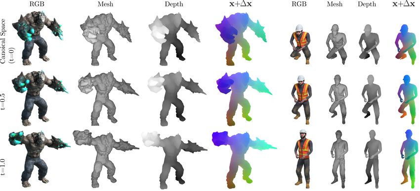
from-Motion [14, 41, 38], light-field photography [18] and       2. Related work
image-based rendering approaches [5]. For instance, the
Neural Radiance Fields (NeRF) [26] have shown that sim-          Neural implicit representation for 3D geometry. The
ple multilayer perceptron networks can encode the mapping        success of deep learning on the 2D domain has spurred a
from 5D inputs (representing spatial locations (x, y, z) and     growing interest in the 3D domain. Nevertheless, which
camera views (θ, φ)) to emitted radiance values and volume       is the most appropriate 3D data representation for deep
density. This learned mapping allows then free-viewpoint         learning remains an open question, especially for non-
rendering with extraordinary realism. Subsequent works           rigid geometry. Standard representations for rigid geome-
have extended Neural Radiance Fields to images in the wild       try include point-clouds [42, 33], voxels [13, 48] and oc-
undergoing severe lighting changes [23] and have proposed        trees [45, 39]. Recently, there has been a strong burst in
sparse voxel fields for rapid inference [19]. Similar schemes    representing 3D data in an implicit manner via a neural net-
have also been recently used for multi-view surface recon-       work [24, 31, 6, 47, 8, 12]. The main idea behind this ap-
struction [50] and learning surface light fields [30].           proach is to describe the information (e.g. occupancy, dis-
                                                                 tance to surface, color, illumination) of a 3D point x as the
    Nevertheless, all these approaches assume a static scene     output of a neural network f (x). Compared to the previ-
without moving objects. In this paper we relax this assump-      ously mentioned representations, neural implicit represen-
tion and propose, to the best of our knowledge, the first end-   tations allow for continuous surface reconstruction at a low
to-end neural rendering system that is applicable to dynamic     memory footprint.
scenes, made of both still and moving/deforming objects.             The first works exploiting implicit representations [24,
While there exist approaches for 4D view synthesis [2], our      31, 6, 47] for 3D representation were limited by their re-
approach is different in that: 1) we only require a single       quirement of having access to 3D ground-truth geometry,
camera; 2) we do not need to pre-compute a 3D reconstruc-        often expensive or even impossible to obtain for in the
tion; and 3) our approach can be trained end-to-end.             wild scenes. Subsequent works relaxed this requirement
    Our idea is to represent the input of our system with        by introducing a differentiable render allowing 2D super-
a continuous 6D function, which besides 3D location and          vision. For instance, [20] proposed an efficient ray-based
camera view, it also considers the time component t.             field probing algorithm for efficient image-to-field supervi-
Naively extending NeRF to learn a mapping from (x, y, z, t)      sion. [29, 49] introduced an implicit-based method to cal-
to density and radiance does not produce satisfying results,     culate the exact derivative of a 3D occupancy field surface
as the temporal redundancy in the scene is not effectively       intersection with a camera ray. In [37], a recurrent neu-
exploited. Our observation is that objects can move and          ral network was used to ray-cast the scene and estimate the
deform, but typically do not appear or disappear. Inspired       surface geometry. However, despite these techniques have
by classical 3D scene flow [44], the core idea to build our      a great potential to represent 3D shapes in an unsupervised
method, denoted Dynamic-NeRF (D-NeRF in short), is to            manner, they are typically limited to relatively simple ge-
decompose learning in two modules. The first one learns a        ometries.
spatial mapping (x, y, z, t) → (∆x, ∆y, ∆z) between each             NeRF [26] showed that by implicitly representing a rigid
point of the scene at time t and a canonical scene config-       scene using 5D radiance fields makes it possible to capture
uration. The second module regresses the scene radiance          high-resolution geometry and photo-realistically rendering
emitted in each direction and volume density given the tu-       novel views. [23] extended this method to handle variable
ple (x + ∆x, y + ∆y, z + ∆z, θ, φ). Both mappings are            illumination and transient occlusions to deal with in the wild
learned with deep fully connected networks without convo-        images. In [19], even more complex 3D surfaces were rep-
lutional layers. The learned model then allows to synthesize     resented by using voxel-bouded implicit fields. And [50]
novel images, providing control in the continuum (θ, φ, t)       circumvented the need of multiview camera calibration.
of the camera views and time component, or equivalently,             However, while all mentioned methods achieve impres-
the dynamic state of the scene (see Fig. 1).                     sive results on rigid scenes, none of them can deal with dy-
    We thoroughly evaluate D-NeRF on scenes undergoing           namic and deformable scenes. Occupancy flow [28] was the
very different types of deformation, from articulated mo-        first work to tackle non-rigid geometry by learning continu-
tion to humans performing complex body poses. We show            ous vector field assigning a motion vector to every point in
that by decomposing learning into a canonical scene and          space and time, but it requires full 3D ground-truth super-
scene flow D-NeRF is able to render high-quality images          vision. Neural volumes [21] produced high quality recon-
while controlling both camera view and time components.          struction results via an encoder-decoder voxel-based repre-
As a side-product, our method is also able to produce com-       sentation enhanced with an implicit voxel warp field, but
plete 3D meshes that capture the time-varying geometry and       they require a muti-view image capture setting.
which remarkably are obtained by observing the scene un-             To the best of our knowledge, D-NeRF is the first ap-
der a specific deformation only from one single viewpoint.       proach able to generate a neural implicit representation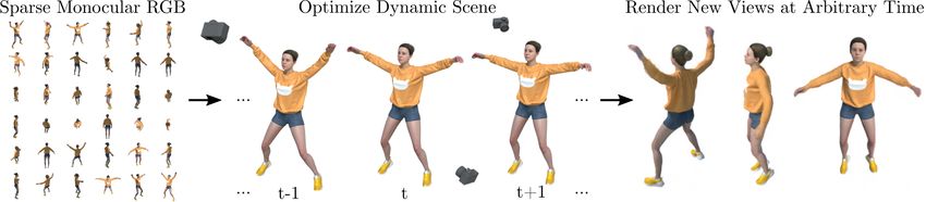
Figure 2: Problem Definition. Given a sparse set of images of a dynamic scene moving non-rigidly and being captured by a monocular
camera, we aim to design a deep learning model to implicitly encode the scene and synthesize novel views at an arbitrary time. Here,
we visualize a subset of the input training frames paired with accompanying camera parameters, and we show three novel views at three
different time instances rendered by the proposed method.
for non-rigid and time-varying scenes, trained solely on             render novel views. Nevertheless, by decoupling depth es-
monocular data without the need of 3D ground-truth super-            timation from novel view synthesis, the outcome of this
vision nor a multi-view camera setting.                              approach becomes highly dependent on the quality of the
                                                                     depth maps as well as on the reliability of the optical flow.
Novel view synthesis. Novel view synthesis is a long                 Very recently, X-Fields [4] introduced a neural network
standing vision and graphics problem that aims to synthe-            to interpolate between images taken across different view,
size new images from arbitrary view points of a scene cap-           time or illumination conditions. However, while this ap-
tured by multiple images. Most traditional approaches for            proach is able to process dynamic scenes, it requires more
rigid scenes consist on reconstructing the scene from multi-         than one view. Since no 3D representation is learned, vari-
ple views with Structure-from-Motion [14] and bundle ad-             ation in viewpoint is small.
justment [41], while other approaches propose light-field               D-NeRF is different from all prior work in that it does
based photography [18]. More recently, deep learning based           not require 3D reconstruction, can be learned end-to-end,
techniques [36, 16, 10, 9, 25] are able to learn a neural vol-       and requires a single view per time instance. Another ap-
umetric representation from a set of sparse images.                  pealing characteristic of D-NeRF is that it inherently learns
   However, none of these methods can synthesize novel               a time-varying 3D volume density and emitted radiance,
views of dynamic scenes. To tackle non-rigid scenes most             which turns the novel view synthesis into a ray-casting pro-
methods approach the problem by reconstructing a dynamic             cess instead of a view interpolation, which is remarkably
3D textured mesh. 3D reconstruction of non-rigid sur-                more robust to rendering images from arbitrary viewpoints.
faces from monocular images is known to be severely ill-
posed. Structure-from-Template (SfT) approaches [3, 7, 27]           3. Problem Formulation
recover the surface geometry given a reference known
template configuration. Temporal information is another                  Given a sparse set of images of a dynamic scene captured
prior typically exploited. Non-rigid-Structure-from-Motion           with a monocular camera, we aim to design a deep learning
(NRSfM) techniques [40, 1] exploit temporal information.             model able to implicitly encode the scene and synthesize
Yet, SfT and NRSfM require either 2D-to-3D matches or                novel views at an arbitrary time (see Fig. 2).
2D point tracks, limiting their general applicability to rela-           Formally, our goal is to learn a mapping M that, given
tively well-textured surfaces and mild deformations.                 a 3D point x = (x, y, z), outputs its emitted color c =
   Some of these limitations are overcome by learning                (r, g, b) and volume density σ conditioned on a time instant
based techniques, which have been effectively used for syn-          t and view direction d = (θ, φ). That is, we seek to estimate
thesizing novel photo-realistic views of dynamic scenes.             the mapping M : (x, d, t) → (c, σ).
For instance, [2, 54, 15] capture the dynamic scene at the               An intuitive solution would be to directly learn the trans-
same time instant from multiple views, to then generate 4D           formation M from the 6D space (x, d, t) to the 4D space
space-time visualizations. [11, 32, 53] also leverage on si-         (c, σ). However, as we will show in the results section, we
multaneously capturing the scene from multiple cameras to            obtain consistently better results by splitting the mapping M
estimate depth, completing areas with missing information            into Ψx and Ψt , where Ψx represents the scene in canoni-
and then performing view synthesis. In [51], the need of             cal configuration and Ψt a mapping between the scene at
multiple views is circumvented by using a pre-trained net-           time instant t and the canonical one. More precisely, given
work that estimates a per frame depth. This depth, jointly           a point x and viewing direction d at time instant t we first
with the optical flow and consistent depth estimation across         transform the point position to its canonical configuration
frames, are then used to interpolate between images and              as Ψt : (x, t) → ∆x. Without loss of generality, we chose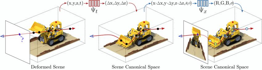
Figure 3: D-NeRF Model. The proposed architecture consists of two main blocks: a deformation network Ψt mapping all scene
deformations to a common canonical configuration; and a canonical network Ψx regressing volume density and view-dependent RGB
color from every camera ray.
t = 0 as the canonical scene Ψt : (x, 0) → 0. By doing so        4.1. Model Architecture
the scene is no longer independent between time instances,
and becomes interconnected through a common canonical            Canonical Network. With the use of a canonical config-
space anchor. Then, the assigned emitted color and vol-          uration we seek to find a representation of the scene that
ume density under viewing direction d equal to those in the      brings together the information of all corresponding points
canonical configuration Ψx : (x + ∆x, d) → (c, σ).               in all images. By doing this, the missing information from a
    We propose to learn Ψx and Ψt using a sparse set of T        specific viewpoint can then be retrieved from that canonical
RGB images {It , Tt }Tt=1 captured with a monocular cam-         configuration, which shall act as an anchor interconnecting
era, where It ∈ RH×W ×3 denotes the image acquired un-           all images.
der camera pose Tt ∈ R4×4 SE(3), at time t. Although                 The canonical network Ψx is trained so as to encode vol-
we could assume multiple views per time instance, we want        umetric density and color of the scene in canonical config-
to test the limits of our method, and assume a single image      uration. Concretely, given the 3D coordinates x of a point,
per time instance. That is, we do not observe the scene un-      we first encode it into a 256-dimensional feature vector.
der a specific configuration/deformation state from different    This feature vector is then concatenated with the camera
viewpoints.                                                      viewing direction d, and propagated through a fully con-
                                                                 nected layer to yield the emitted color c and volume density
4. Method                                                        σ for that given point in the canonical space.
                                                                 Deformation Network. The deformation network Ψt is op-
    We now introduce D-NeRF, our novel neural renderer for       timized to estimate the deformation field between the scene
view synthesis trained solely from a sparse set of images of     at a specific time instant and the scene in canonical space.
a dynamic scene. We build on NeRF [26] and generalize it         Formally, given a 3D point x at time t, Ψt is trained to out-
to handle non-rigid scenes. Recall that NeRF requires mul-       put the displacement ∆x that transforms the given point to
tiple views of a rigid scene In contrast, D-NeRF can learn a     its position in the canonical space as x + ∆x. For all ex-
volumetric density representation for continuous non-rigid       periments, without loss of generality, we set the canonical
scenes trained with a single view per time instant.              scene to be the scene at time t = 0:
    As shown in Fig. 3, D-NeRF consists of two main neu-
ral network modules, which parameterize the mappings ex-
                                                                                              (
                                                                                                  ∆x, if t 6= 0
plained in the previous section Ψt , Ψx . On the one hand we                    Ψt (x, t) =                               (1)
have the Canonical Network, an MLP (multilayer percep-                                            0,  if t = 0
tron) Ψx (x, d) 7→ (c, σ) is trained to encode the scene in
the canonical configuration such that given a 3D point x and         As shown in previous works [34, 43, 26], directly feed-
a view direction d returns its emitted color c and volume        ing raw coordinates and angles to a neural network results in
density σ. The second module is called Deformation Net-          low performance. Thus, for both the canonical and the de-
work and consists of another MLP Ψt (x, t) 7→ ∆x which           formation networks, we first encode x, d and t into a higher
predicts a deformation field defining the transformation be-     dimension space. We use the same positional encoder as
tween the scene at time t and the scene in its canonical         in [26] where γ(p) =< (sin(2l πp), cos(2l πp)) >L 0 . We in-
configuration. We next describe in detail each one of these      dependently apply the encoder γ(·) to each coordinate and
blocks (Sec. 4.1), their interconnection for volume render-      camera view component, using L = 10 for x, and L = 4
ing (Sec. 4.2) and how are they learned (Sec. 4.3).              for d and t.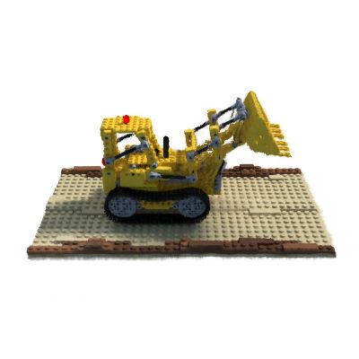
4.2. Volume Rendering                                                    squared error between the rendered and real pixels:
   We now adapt NeRF volume rendering equations to ac-                                       Ns
                                                                                                                         2
                                                                                          1 X
count for non-rigid deformations in the proposed 6D neural                           L=          Ĉ(p, t) − C 0 (p, t)            (9)
                                                                                          Ns i=1                         2
radiance field. Let x(h) = o+hd be a point along the cam-
era ray emitted from the center of projection o to a pixel p.
Considering near and far bounds hn and hf in that ray, the               where Ĉ are the pixels’ ground-truth color.
expected color C of the pixel p at time t is given by:
                                                                         5. Implementation Details
                 Z   hf
   C(p, t) =              T(h, t)σ(p(h, t))c(p(h, t), d)dh,       (2)        Both the canonical network Ψx and the deformation net-
                  hn                                                     work Ψt consists on simple 8-layers MLPs with ReLU ac-
      where p(h, t) = x(h) + Ψt (x(h), t),                        (3)    tivations. For the canonical network a final sigmoid non-
                                                                         linearity is applied to c and σ. No non-linearlity is applied
     [c(p(h, t), d), σ(p(h, t))] = Ψx (p(h, t), d),               (4)
                               Z h              !                        to ∆x in the deformation network.
                                                                             For all experiments we set the canonical configuration
      and T(h, t) = exp −          σ(p(s, t))ds .                 (5)
                                      hn                                 as the scene state at t = 0 by enforcing it in Eq. (1). To
                                                                         improve the networks convergence, we sort the input im-
The 3D point p(h, t) denotes the point on the camera ray                 ages according to their time stamps (from lower to higher)
x(h) transformed to canonical space using our Deformation                and then we apply a curriculum learning strategy where we
Network Ψt , and T(h, t) is the accumulated probability that             incrementally add images with higher time stamps.
the ray emitted from hn to hf does not hit any other particle.               The model is trained with 400 × 400 images during 800k
Notice that the density σ and color c are predicted by our               iterations with a batch size of Ns = 4096 rays, each sam-
Canonical Network Ψx .                                                   pled 64 times along the ray. As for the optimizer, we
   As in [26] the volume rendering integrals in Eq. (2)                  use Adam [17] with learning rate of 5e − 4, β1 = 0.9,
and Eq. (5) can be approximated via numerical quadrature.                β2 = 0.999 and exponential decay to 5e − 5. The model
To select a random set of quadrature points {hn }N                       is trained with a single Nvidia® GTX 1080 for 2 days.
                                                      n=1 ∈
[hn , hf ] a stratified sampling strategy is applied by uni-
formly drawing samples from evenly-spaced ray bins. A                    6. Experiments
pixel color is approximated as:                                              This section provides a thorough evaluation of our sys-
                                                                         tem. We first test the main components of the model,
                 N
                 X                                                       namely the canonical and deformation networks (Sec. 6.1).
  C 0 (p, t) =         T 0 (hn , t)α(hn , t, δn )c(p(hn , t), d), (6)    We then compare D-NeRF against NeRF and T-NeRF,
                 n=1
                                                                         a variant in which does not use the canonical mapping
    where α(h, t, δ) = 1 − exp(−σ(p(h, t))δ),                     (7)    (Sec. 6.2). Finally, we demonstrate D-NeRF ability to syn-
                                      n−1
                                                             !
                                      X                                  thesize novel views at an arbitrary time in several complex
     and   T 0 (hn , t) = exp −             σ(p(hm , t))δm       , (8)   dynamic scenes (Sec. 6.3).
                                      m=1                                    In order to perform an exhaustive evaluation we have ex-
                                                                         tended NeRF [26] rigid benchmark with eight scenes con-
and δn = hn+1 −hn is the distance between two quadrature
                                                                         taining dynamic objects under large deformations and real-
points.
                                                                         istic non-Lambertian materials. As in the rigid benchmark
                                                                         of [26], six are rendered from viewpoints sampled from the
4.3. Learning the Model
                                                                         upper hemisphere, and two are rendered from viewpoints
   The parameters of the canonical Ψx and deformation                    sampled on the full sphere. Each scene contains between
Ψt networks are simultaneously learned by minimizing the                 100 and 200 rendered views depending on the action time
mean squared error with respect to the T RGB images                      span, all at 800 × 800 pixels. We will release the path-
{It }Tt=1 of the scene and their corresponding camera pose               traced images with defined train/validation/test splits for
matrices {Tt }Tt=1 . Recall that every time instant is only              these eight scenes.
acquired by a single camera.
                                                                         6.1. Dissecting the Model
   At each training batch, we first sample a random set of
pixels {pt,i }N s
              i=1 corresponding to the rays cast from some                  This subsection provides insights about D-NeRF be-
camera position Tt to some pixels i of the corresponding                 haviour when modeling a dynamic scene and analyze the
RGB image t. We then estimate the colors of the chosen                   two main modules, namely the canonical and deformation
pixels using Eq. (6). The training loss we use is the mean               networks.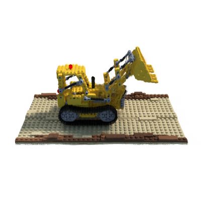
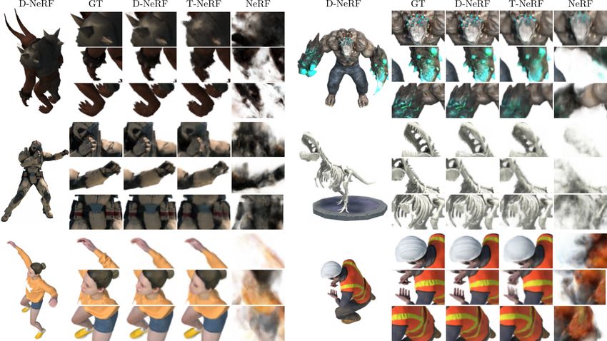
Figure 4: Visualization of the Learned Scene Representation. From left to right: the learned radiance from a specific viewpoint,
the volume density represented as a 3D mesh and a depth map, and the color-coded points of the canonical configuration mapped to the
deformed meshes based on ∆x. The same colors on corresponding points indicate the correctness of such mapping.
       t=0.5            Canonical Space             t=1             at mapped to the different shape configurations at t = 0.5
                                                                    and t = 1. Note that the colors consistency along time,
                                                                    indicating that the displacement field is correctly estimated.
                                                                       Another question that we try to answer is how D-NeRF
                                                                    manages to model phenomena like shadows/shading ef-
Figure 5: Analyzing Shading Effects. Pairs of corresponding         fects, that is, how the model can encode changes of ap-
points between the canonical space and the scene at times t = 0.5   pearance of the same point along time. We have carried
and t = 1.                                                          an additional experiment to answer this. In Fig. 5 we show
   We initially evaluate the ability of the canonical network       a scene with three balls, made of very different materials
to represent the scene in a canonical configuration. The re-        (plastic –green–, translucent glass –blue– and metal –red–).
sults of this analysis for two scenes are shown the first row       The figure plots pairs of corresponding points between the
of Fig. 4 (columns 1-3 in each case). The plots show, for           canonical configuration and the scene at a specific time in-
the canonical configuration (t = 0), the RGB image, the 3D          stant. D-NeRF is able to synthesize the shading effects by
occupancy network and the depth map, respectively. The              warping the canonical configuration. For instance, observe
rendered RGB image is the result of evaluating the canoni-          how the floor shadows are warped along time. Note that the
cal network on rays cast from an arbitrary camera position          points in the shadow of, e.g. the red ball, at t = 0.5 and
applying Eq. (6). To better visualize the learned volumet-          t = 1 map at different regions of the canonical space.
ric density we transform it into a mesh applying marching
                                                                    6.2. Quantitative Comparison
cubes [22], with a 3D cube resolution of 2563 voxels. Note
how D-NeRF is able to model fine geometric and appear-                 We next evaluate the quality of D-NeRF on the novel
ance details for complex topologies and texture patterns,           view synthesis problem and compare it against the origi-
even when it was only trained with a set of sparse images,          nal NeRF [26], which represents the scene using a 5D in-
each under a different deformation.                                 put (x, y, z, θ, φ), and T-NeRF, a straight-forward exten-
   In a second experiment we assess the capacity of the net-        sion of NeRF in which the scene is represented by a 6D
work to estimate consistent deformation fields that map the         input (x, y, z, θ, φ, t), without considering the intermediate
canonical scene to the particular shape at each input image.        canonical configuration of D-NeRF.
The second and third rows of Fig. 4 show the result of ap-             Table 1 summarizes the quantitative results on the 8 dy-
plying the corresponding translation vectors to the canon-          namic scenes of our dataset. We use several metrics for
ical space for t = 0.5 and t = 1. The fourth column in              the evaluation: Mean Squared Error (MSE), Peak Signal-to-
each of the two examples visualizes the displacement field,         Noise Ratio (PSNR), Structural Similarity (SSIM) [46] and
where the color-coded points in the canonical shape (t = 0)         Learned Perceptual Image Patch Similarity (LPIPS) [52].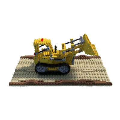
Figure 6: Qualitative Comparison. Novel view synthesis results of dynamic scenes. For every scene we show an image synthesised
from a novel view at an arbitrary time by our method, and three close-ups for: ground-truth, NeRF, T-NeRF, and D-NeRF (ours).

                Hell Warrior             Mutant                   Hook                 Bouncing Balls
Method   MSE↓ PSNR↑ SSIM↑ LPIPS↓ MSE↓ PSNR↑ SSIM↑ LPIPS↓ MSE↓ PSNR↑ SSIM↑ LPIPS↓ MSE↓ PSNR↑ SSIM↑ LPIPS↓
NeRF   44e-3   13.52   0.81 0.25 9e-4  20.31   0.91 0.09                   21e-316.65    0.84 0.19       94e-4 20.26    0.91   0.2
T-NeRF 47e-4   23.19   0.93 0.08 8e-4  30.56   0.96 0.04                   18e-427.21    0.94 0.06       16e-5 37.81    0.98  0.12
D-NeRF 31e-4   25.02   0.95 0.06 7e-4  31.29   0.97 0.02                   11e-429.25    0.96 0.11       12e-5 38.93    0.98   0.1
                    Lego                   T-Rex                                   Stand Up                     Jumping Jacks
Method   MSE↓ PSNR↑ SSIM↑ LPIPS↓ MSE↓ PSNR↑ SSIM↑ LPIPS↓                  MSE↓ PSNR↑ SSIM↑ LPIPS↓        MSE↓ PSNR↑ SSIM↑ LPIPS↓
NeRF      9e-3   20.30   0.79    0.23    3e-3   24.49   0.93      0.13     1e-2    18.19   0.89   0.14   1e-2    18.28   0.88   0.23
T-NeRF    3e-4   23.82   0.90    0.15    9e-3   30.19   0.96      0.13     7e-4    31.24   0.97   0.02   6e-4    32.01   0.97   0.03
D-NeRF    6e-4   21.64   0.83    0.16    6e-3   31.75   0.97      0.03     5e-4    32.79   0.98   0.02   5e-4    32.80   0.98   0.03

           Table 1: Quantitative Comparison. We report MSE/LPIPS (lower is better) and PSNR/SSIM (higher is better).
In Fig. 6 we show samples of the estimated images under                  (Fig. 7). The first column displays the canonical config-
a novel view for visual inspection. As expected, NeRF is                 uration. Note that we are able to handle several types of
not able to model the dynamics scenes as it was designed                 dynamics: articulated motion in the Tractor scene; human
for rigid cases, always converging to a blurry mean repre-               motion in the Jumping Jacks and Warrior scenes; and asyn-
sentation of all deformations. On the other hand, T-NeRF                 chronous motion of several Bouncing Balls. Also note that
baseline is able to capture reasonably well the dynamics, al-            the canonical configuration is a sharp and neat scene, in all
though is not able to retrieve high frequency details. For ex-           cases, expect for the Jumping Jacks, where the two arms
ample, in Fig. 6 top-left image it fails to encode the shoulder          appear to be blurry. This, however, does not harm the qual-
pad spikes, and in the top-right scene it is not able to model           ity of the rendered images, indicating that the network is
the stones and cracks. D-NeRF, instead, retains high details             able warp the canonical configuration so as to maximize the
of the original image in the novel views. This is quite re-              rendering quality. This is indeed consistent with Sec. 6.1
markable, considering that each deformation state has only               insights on how the network is able to encode shading.
been seen from a single viewpoint.                                          D-NeRF has two main failure cases: (i) Poor camera
                                                                         poses (as in NeRF). (ii) Large deformations between tem-
6.3. Additional Results
                                                                         porally consecutive input images prevents the model from
   We finally show additional results to showcase the wide               converging to a consistent deformation field. This can be
range of scenarios that can be handled with D-NeRF                       solved by increasing the capture frame rate.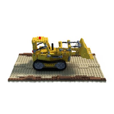
Canonical Space              t=0.1                 t=0.3                  t=0.5                    t=0.8                    t=1.0

Figure 7: Time & View Conditioning. Results of synthesising diverse scenes from two novel points of view across time and the learned
canonical space. For every scene we also display the learned scene canonical space in the first column.

7. Conclusion                                                        ation demonstrates that D-NeRF is able to synthesise high
   We have presented D-NeRF, a novel neural radiance field           quality novel views of scenes undergoing different types of
approach for modeling dynamic scenes. Our method can                 deformation, from articulated objects to human bodies per-
be trained end-to-end from only a sparse set of images ac-           forming complex body postures.
quired with a moving camera, and does not require pre-
computed 3D priors nor observing the same scene config-              Acknowledgments This work is supported in part by a Google
uration from different viewpoints. The main idea behind D-           Daydream Research award and by the Spanish government with the project
NeRF is to represent time-varying deformations with two              HuMoUR TIN2017-90086-R, the ERA-Net Chistera project IPALM
                                                                     PCI2019-103386 and Marı́a de Maeztu Seal of Excellence MDM-2016-
modules: one that learns a canonical configuration, and an-          0656. Gerard Pons-Moll is funded by the Deutsche Forschungsgemein-
other that learns the displacement field of the scene at each        schaft (DFG, German Research Foundation) - 409792180 (Emmy Noether
time instant w.r.t. the canonical space. A thorough evalu-           Programme, project: Real Virtual Humans).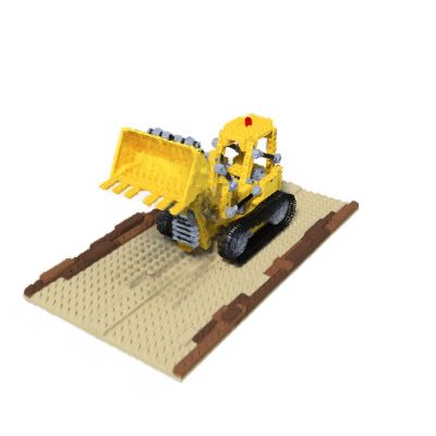
References                                                          [19] Lingjie Liu, Jiatao Gu, Kyaw Zaw Lin, Tat-Seng Chua,
                                                                         and Christian Theobalt. Neural sparse voxel fields. arXiv
 [1] Antonio Agudo and Francesc Moreno-Noguer. Simultaneous              preprint arXiv:2007.11571, 2020. 1, 2
     pose and non-rigid shape with particle dynamics. In CVPR,      [20] Shichen Liu, Shunsuke Saito, Weikai Chen, and Hao Li.
     2015. 3                                                             Learning to infer implicit surfaces without 3d supervision.
 [2] Aayush Bansal, Minh Vo, Yaser Sheikh, Deva Ramanan, and             In NeurIPS, 2019. 2
     Srinivasa Narasimhan. 4d visualization of dynamic events       [21] Stephen Lombardi, Tomas Simon, Jason Saragih, Gabriel
     from unconstrained multi-view videos. In CVPR, 2020. 2, 3           Schwartz, Andreas Lehrmann, and Yaser Sheikh. Neural vol-
 [3] Adrien Bartoli, Yan Gérard, Francois Chadebecq, Toby               umes: learning dynamic renderable volumes from images.
     Collins, and Daniel Pizarro. Shape-from-template. T-PAMI,           TOG, 38(4), 2019. 2
     37(10), 2015. 3                                                [22] William E Lorensen and Harvey E Cline. Marching cubes:
 [4] Mojtaba Bemana, Karol Myszkowski, Hans-Peter Seidel,                A high resolution 3d surface construction algorithm. SIG-
     and Tobias Ritschel. X-fields: Implicit neural view-, light-        GRAPH, 1987. 6
     and time-image interpolation. TOG, 39(6), 2020. 3              [23] Ricardo Martin-Brualla, Noha Radwan, Mehdi SM Sajjadi,
 [5] Chris Buehler, Michael Bosse, Leonard McMillan, Steven              Jonathan T Barron, Alexey Dosovitskiy, and Daniel Duck-
     Gortler, and Michael Cohen. Unstructured lumigraph ren-             worth. Nerf in the wild: Neural radiance fields for uncon-
     dering. In SIGGRAPH, 2001. 2                                        strained photo collections. arXiv preprint arXiv:2008.02268,
 [6] Zhiqin Chen and Hao Zhang. Learning implicit fields for             2020. 1, 2
     generative shape modeling. In CVPR, 2019. 2                    [24] Lars Mescheder, Michael Oechsle, Michael Niemeyer, Se-
 [7] Ajad Chhatkuli, Daniel Pizarro, and Adrien Bartoli. Sta-            bastian Nowozin, and Andreas Geiger. Occupancy networks:
     ble template-based isometric 3d reconstruction in all imag-         Learning 3d reconstruction in function space. In CVPR,
     ing conditions by linear least-squares. In CVPR, 2014. 3            2019. 2
 [8] Julian Chibane, Thiemo Alldieck, and Gerard Pons-Moll.         [25] Ben Mildenhall, Pratul P. Srinivasan, Rodrigo Ortiz-Cayon,
     Implicit functions in feature space for 3d shape reconstruc-        Nima Khademi Kalantari, Ravi Ramamoorthi, Ren Ng, and
     tion and completion. In Proceedings of the IEEE/CVF Con-            Abhishek Kar. Local light field fusion: Practical view syn-
     ference on Computer Vision and Pattern Recognition, pages           thesis with prescriptive sampling guidelines. TOG, 2019. 3
     6970–6981, 2020. 2                                             [26] Ben Mildenhall, Pratul P Srinivasan, Matthew Tancik,
 [9] Inchang Choi, Orazio Gallo, Alejandro Troccoli, Min H               Jonathan T Barron, Ravi Ramamoorthi, and Ren Ng. Nerf:
     Kim, and Jan Kautz. Extreme view synthesis. In CVPR,                Representing scenes as neural radiance fields for view syn-
     2019. 3                                                             thesis. arXiv preprint arXiv:2003.08934, 2020. 1, 2, 4, 5,
[10] John Flynn, Michael Broxton, Paul Debevec, Matthew Du-              6
     Vall, Graham Fyffe, Ryan Overbeck, Noah Snavely, and           [27] F. Moreno-Noguer and P. Fua. Stochastic exploration of am-
     Richard Tucker. Deepview: View synthesis with learned gra-          biguities for nonrigid shape recovery. T-PAMI, 35(2), 2013.
     dient descent. In CVPR, 2019. 3                                     3
                                                                    [28] Michael Niemeyer, Lars Mescheder, Michael Oechsle, and
[11] John Flynn, Ivan Neulander, James Philbin, and Noah
                                                                         Andreas Geiger. Occupancy flow: 4d reconstruction by
     Snavely. Deepstereo: Learning to predict new views from
                                                                         learning particle dynamics. In ICCV, 2019. 2
     the world’s imagery. In CVPR, 2016. 3
                                                                    [29] Michael Niemeyer, Lars Mescheder, Michael Oechsle, and
[12] Kyle Genova, Forrester Cole, Avneesh Sud, Aaron Sarna,
                                                                         Andreas Geiger. Differentiable volumetric rendering: Learn-
     and Thomas Funkhouser. Local deep implicit functions for
                                                                         ing implicit 3d representations without 3d supervision. In
     3d shape. In Proceedings of the IEEE/CVF Conference
                                                                         CVPR, 2020. 1, 2
     on Computer Vision and Pattern Recognition, pages 4857–
                                                                    [30] Michael Oechsle, Michael Niemeyer, Lars Mescheder, Thilo
     4866, 2020. 2
                                                                         Strauss, and Andreas Geiger. Learning implicit surface light
[13] Rohit Girdhar, David F Fouhey, Mikel Rodriguez, and Ab-             fields. arXiv preprint arXiv:2003.12406, 2020. 2
     hinav Gupta. Learning a predictable and generative vector
                                                                    [31] Jeong Joon Park, Peter Florence, Julian Straub, Richard
     representation for objects. In ECCV, 2016. 2
                                                                         Newcombe, and Steven Lovegrove. Deepsdf: Learning con-
[14] Richard Hartley and Andrew Zisserman. Multiple view ge-             tinuous signed distance functions for shape representation.
     ometry in computer vision. Cambridge university press,              In CVPR, 2019. 2
     2003. 2, 3                                                     [32] Julien Philip and George Drettakis. Plane-based multi-view
[15] Hanqing Jiang, Haomin Liu, Ping Tan, Guofeng Zhang, and             inpainting for image-based rendering in large scenes. In SIG-
     Hujun Bao. 3d reconstruction of dynamic scenes with mul-            GRAPH, 2018. 3
     tiple handheld cameras. In ECCV, 2012. 3                       [33] Albert Pumarola, Stefan Popov, Francesc Moreno-Noguer,
[16] Abhishek Kar, Christian Häne, and Jitendra Malik. Learning         and Vittorio Ferrari. C-flow: Conditional generative flow
     a multi-view stereo machine. In NeurIPS, 2017. 3                    models for images and 3d point clouds. In CVPR, 2020. 2
[17] Diederik Kingma and Jimmy Ba. ADAM: A method for               [34] Nasim Rahaman, Aristide Baratin, Devansh Arpit, Felix
     stochastic optimization. In ICLR, 2015. 5                           Draxler, Min Lin, Fred Hamprecht, Yoshua Bengio, and
[18] Marc Levoy and Pat Hanrahan. Light field rendering. In              Aaron Courville. On the spectral bias of neural networks.
     SIGGRAPH, 1996. 2, 3                                                In ICML, 2019. 4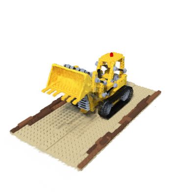
[35] Konstantinos Rematas and Vittorio Ferrari. Neural voxel ren-            with globally coherent depths from a monocular camera. In
     derer: Learning an accurate and controllable rendering tool.            CVPR, 2020. 3
     In CVPR, 2020. 1                                                   [52] Richard Zhang, Phillip Isola, Alexei A Efros, Eli Shechtman,
[36] Liyue Shen, Wei Zhao, and Lei Xing. Patient-specific recon-             and Oliver Wang. The unreasonable effectiveness of deep
     struction of volumetric computed tomography images from a               features as a perceptual metric. In CVPR, 2018. 6
     single projection view via deep learning. Nature biomedical        [53] Tinghui Zhou, Richard Tucker, John Flynn, Graham Fyffe,
     engineering, 3(11), 2019. 3                                             and Noah Snavely. Stereo magnification: learning view syn-
[37] Vincent Sitzmann, Michael Zollhöfer, and Gordon Wet-                   thesis using multiplane images. TOG, 37(4), 2018. 3
     zstein. Scene representation networks: Continuous 3d-              [54] C Lawrence Zitnick, Sing Bing Kang, Matthew Uyttendaele,
     structure-aware neural scene representations. In NeurIPS,               Simon Winder, and Richard Szeliski. High-quality video
     2019. 2                                                                 view interpolation using a layered representation. TOG,
[38] Noah Snavely, Steven M Seitz, and Richard Szeliski. Photo               23(3), 2004. 3
     tourism: exploring photo collections in 3d. In SIGGRAPH,
     2006. 2
[39] Maxim Tatarchenko, Alexey Dosovitskiy, and Thomas Brox.
     Octree Generating Networks: Efficient Convolutional Archi-
     tectures for High-resolution 3D Outputs. In ICCV, 2017. 2
[40] Carlo Tomasi and Takeo Kanade. Shape and motion from
     image streams under orthography: a factorization method.
     IJCV, 9(2), 1992. 3
[41] Bill Triggs, Philip F McLauchlan, Richard I Hartley, and An-
     drew W Fitzgibbon. Bundle adjustment—a modern synthe-
     sis. In International workshop on vision algorithms, 1999.
     2, 3
[42] Shubham Tulsiani, Tinghui Zhou, Alexei A Efros, and Jiten-
     dra Malik. A Point Set Generation Network for 3D Object
     Reconstruction from a Single Image. In CVPR, 2017. 2
[43] Ashish Vaswani, Noam Shazeer, Niki Parmar, Jakob Uszko-
     reit, Llion Jones, Aidan N Gomez, Łukasz Kaiser, and Illia
     Polosukhin. Attention is all you need. In NeurIPS, 2017. 4
[44] Sundar Vedula, Peter Rander, Robert Collins, and Takeo
     Kanade. Three-dimensional scene flow. IEEE transactions
     on pattern analysis and machine intelligence, 27(3):475–
     480, 2005. 2
[45] Peng-Shuai Wang, Yang Liu, Yu-Xiao Guo, Chun-Yu Sun,
     and Xin Tong. O-CNN: Octree-based Convolutional Neural
     Networks for 3D Shape Analysis. TOG, 36(4), 2017. 2
[46] Zhou Wang, Alan C Bovik, Hamid R Sheikh, and Eero P
     Simoncelli. Image quality assessment: from error visibility
     to structural similarity. TIP, 13(4), 2004. 6
[47] Qiangeng Xu, Weiyue Wang, Duygu Ceylan, Radomir
     Mech, and Ulrich Neumann. Disn: Deep implicit surface
     network for high-quality single-view 3d reconstruction. In
     NeurIPS, 2019. 2
[48] Xinchen Yan, Jimei Yang, Ersin Yumer, Yijie Guo, and
     Honglak Lee. Perspective Transformer Nets: Learning
     Single-view 3D object Reconstruction without 3D Supervi-
     sion. In NIPS, 2016. 2
[49] Lior Yariv, Matan Atzmon, and Yaron Lipman. Univer-
     sal differentiable renderer for implicit neural representations.
     arXiv preprint arXiv:2003.09852, 2020. 2
[50] Lior Yariv, Yoni Kasten, Dror Moran, Meirav Galun, Matan
     Atzmon, Basri Ronen, and Yaron Lipman. Multiview neu-
     ral surface reconstruction by disentangling geometry and ap-
     pearance. NeurIPS, 2020. 1, 2
[51] Jae Shin Yoon, Kihwan Kim, Orazio Gallo, Hyun Soo Park,
     and Jan Kautz. Novel view synthesis of dynamic scenes
You can also read