David Lowe's recognition system - Lecture 5 - Spring 2005 EE/CNS/CS 148 - P. Perona

David Lowe’s
recognition system

    Lecture 5 - Spring 2005
   EE/CNS/CS 148 - P. Perona

Invariance to translation

Invariance to orientation

            Text

                            3

Invariance to scale

Moreover...
•   Clutter
•   Lighting
•   Occlusion
•   ...

                              5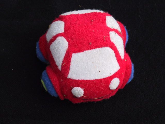

Distinctive Image Features
from Scale-Invariant Keypoints
David G. Lowe
Computer Science Department
University of British Columbia
Vancouver, B.C., Canada
lowe@cs.ubc.ca
January 5, 2004

International Journal of Computer Vision, 2004.

Abstract
This paper presents a method for extracting distinctive invariant features from
images that can be used to perform reliable matching between different views of
an object or scene. The features are invariant to image scale and rotation, and
are shown to provide robust matching across a a substantial range of affine distortion,
change in 3D viewpoint, addition of noise, and change in illumination.
The features are highly distinctive, in the sense that a single feature can be correctly
matched with high probability against a large database of features from
many images. This paper also describes an approach to using these features
for object recognition. The recognition proceeds by matching individual features
to a database of features from known objects using a fast nearest-neighbor
algorithm, followed by a Hough transform to identify clusters belonging to a single
object, and finally performing verification through least-squares solution for
consistent pose parameters. This approach to recognition can robustly identify
objects among clutter and occlusion while achieving near real-time performance.

http://www.cs.ubc.ca/~lowe/papers/ijcv04.pdf

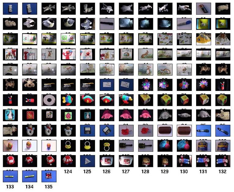
Database of individual objects

Interest points detector

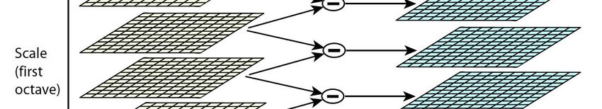
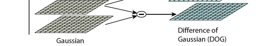
                  Difference of gaussians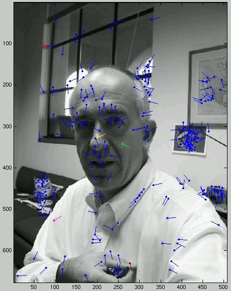

Figure 1: For each octave of scale space, the initial image is repeatedly convolved with Gaussians to
produce the set of scale space images shown on the left. Adjacent Gaussian images are subtracted
to produce the difference-of-Gaussian images on the right. After each octave, the Gaussian image is
down-sampled by a factor of 2, and the process repeated.

+
-

Detection & scale of features

Figure 2: Maxima and minima of the difference-of-Gaussian images are detected by comparing a
pixel (marked with X) to its 26 neighbors in 3x3 regions at the current and adjacent scales (marked
with circles).

Sampling of scale
                 Quality                                                  Quantity

Figure 3: The top line of the first graph shows the percent of keypoints that are repeatably detected at
the same location and scale in a transformed image as a function of the number of scales sampled per
octave. The lower line shows the percent of keypoints that have their descriptors correctly matched to
a large database. The second graph shows the total number of keypoints detected in a typical image
as a function of the number of scale samples.

Figure 4: The top line in the graph shows the percent of keypoint locations that are repeatably detected
in a transformed image as a function of the prior image smoothing for the first level of each octave.
The lower line shows the percent of descriptors correctly matched against a large database.

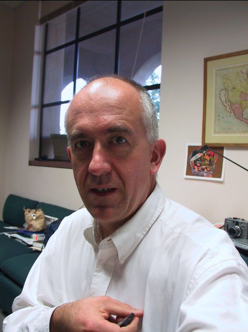
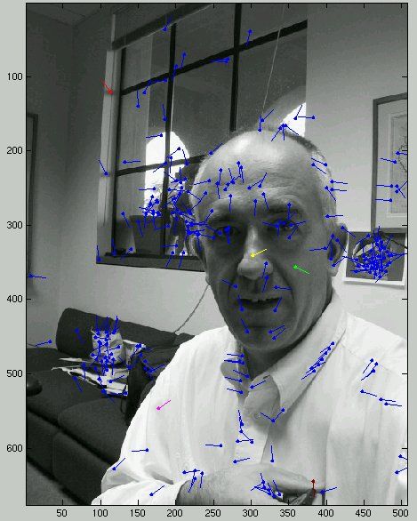
Figure 5: This figure shows the stages of keypoint selection. (a) The 233x189 pixel original image.
(b) The initial 832 keypoints locations at maxima and minima of the difference-of-Gaussian function.
Keypoints are displayed as vectors indicating scale, orientation, and location. (c) After applying
a threshold on minimum contrast, 729 keypoints remain. (d) The final 536 keypoints that remain
following an additional threshold on ratio of principal curvatures.

Choice of descriptors

                  -x, y location
                  -orientation
                  -scale
                  -Description of the local
                  neighborhood by a
                  collection of gradients

SIFT descriptors
                                                                                                  Prevalent orientation

Figure 7: A keypoint descriptor is created by first computing the gradient magnitude and orientation at each image
sample point in a region around the keypoint location, as shown on the left. These are weighted by a Gaussian window,
indicated by the overlaid circle. These samples are then accumulated into orientation histograms summarizing the
contents over 4x4 subregions, as shown on the right, with the length of each arrow corresponding to the sum of the
gradient magnitudes near that direction within the region. This figure shows a 2x2 descriptor array computed from an
8x8 set of samples, whereas the experiments in this paper use 4x4 descriptors computed from a 16x16 sample array.

Stereo system

Matching across images

Matching across viewpoints

    Fraction of stable
    keypoints

Matching across viewpoints

     Fraction of stable
     keypoints

Feature repeatability vs noise

Repeatability vs complexity

Repeatability vs affine distortion

Kd-tree search

  Binary search
                              An exhaustive search is
                              needed to obtain the
                              nearest neighbor. This is
                              time consuming !!

           Nearest neighbor

Kd-tree search - backtracking

Kd-tree search - backtracking

Kd-tree search - backtracking

                            Good choice !

Geometrical consistency
              (x1,y1,s1,θ1
              )(x ,y ,s ,θ
                2   2 2    2
              )
             Transform predicted by this match:
                 •! Δx = x2-x1
                 •! Δy = y2-y1
                 •! Δs = s2 / s1
                 •! Δθ = θ2 / θ1
         ⇒ Voting performed in the space of
           transform parameters
                               Δ
                               s
                    Δ                  Δ
                    θ                  y
                                   Δ
                                   x

Geometrical consistency

                       key

                               g keys
model center
                             matchin

                      key

                                      n
                                tio
                           l oca
                         l
                      de
                    mo
               ed
         ict
    p red

                We look at the space of parameters (Hough transform)
                (localization, orientation, scale ⇒ 4 dimensions)

Lowe’s algorithm at a glance

• Detect features using scale-space DOG
• Compute SIFT descriptors
• Index into feature database
• Enforce pose consistency
• Count votes and declare winner(s)

                                          32

Results: scene recognition

Results: multiple object instances

Recognition in presence of occlusions

Recognition with a change of scale